ISSN 0101-8205 www.scielo.br/cam
Adaptive basis selection for functional data
analysis via stochastic penalization
CEZAR A.F. ANSELMO, RONALDO DIAS and NANCY L. GARCIA
Departamento de Estatística, IMECC, UNICAMP Caixa Postal 6065 – 13081-970 Campinas, SP, Brazil
E-mails: [email protected] / [email protected] / [email protected]
Abstract. We propose an adaptive method of analyzing a collection of curves which can be, individually, modeled as a linear combination of spline basis functions. Through the introduction of latent Bernoulli variables, the number of basis functions, the variance of the error measurements and the coefficients of the expansion are determined. We provide a modification of the stochastic EM algorithm for which numerical results show that the estimates are very close to the true curve in the sense of L2norm.
Mathematical subject classification: Primary: 62G05, Secondary: 65D15.
Key words:basis functions, SEM algorithm, functional statistics, summary measures, splines, non-parametric data analysis, registration.
1 Introduction
It is very common to have data that comes as samples of functions, that is, the data are curves. Such curves can be obtained either from an on-line measuring process, where we have the data collected continuously in time or from a smo-othing process applied to discrete data. Functional Data Analysis (FDA) is a set of techniques that can be used to study the variability of functions from a sample as well as its derivatives. The major goal is to explain the variability within and among the functions. For an extensive discussion of such techniques see Ramsay and Silverman (2002).
In this paper, we assume that each curve can be modeled as a linear combination of B-splines functions. The coefficients of the expansion can be obtained by the least square method. However, in doing so, we get a solution for which the number of basis functions equals the number of observations, achieving interpolation of the data. Interpolation is not desirable since we have noisy data. To avoid this problem we propose a new method to regularize the solution using stochastic penalization. This is possible through the introduction of latent Bernoulli random variables which indicate the subset of basis to be selected and consequently the dimension of the space.
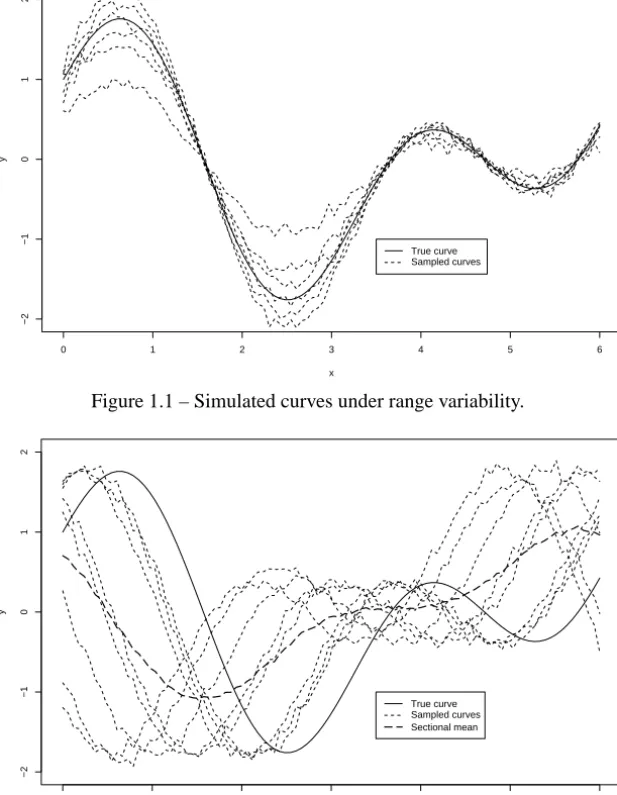
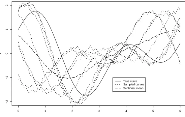
Before applying the model we have to understand the different sources of variability for curves. Variability for functions can be of two types: range and phase. The range variability gives the common pattern to each individual or function. Phase variability, on the other hand, can mask the common pattern of the functions. The usual situation, where both sources of variability are present, require complex estimation techniques. As an example, we can think about height, it is well known that the growth velocity is very high for young children and slows down as the age increases. Different children have different growth velocities in scale (range variation) as well as in time (phase variation). The mean function – also called (cross-)sectional mean – is a descriptive statistic which is widely used to give a rough idea of the process generating the curves. Figures 1.1–1.3 show some examples of variability. Notice in Figure 1.3 that the cross-sectional mean can be very misleading in the presence of phase variability. For all simulated results in this section we used a low variance noise to better illustrate each individual curve.
Our approach, like most approaches in Functional Data Analysis can only be used for curves in the presence of range variability. If phase variability is present it is necessary to align the curves using a method introduced by Ramsay and Li (1998) called registration. After registration is done, we can find the mean of the registered curves – the structural mean. Figure 1.4 presents the same curves as Figure 1.3 after registration. It is clear that in this case the structural mean is much closer to the real curve than the arithmetic sectional mean of the original curves.
0 1 2 3 4 5 6
−2
−1
0
1
2
x
y
True curve Sampled curves
Figure 1.1 – Simulated curves under range variability.
0 1 2 3 4 5 6
−2
−1
0
1
2
x
y
True curve Sampled curves Sectional mean
Figure 1.2 – Simulated curves under phase variability.
0 1 2 3 4 5 6
−2
−1
0
1
2
x
y
True curve Sampled curves Sectional mean
Figure 1.3 – Simulated curves under range and phase variability.
0 1 2 3 4 5 6
−2
−1
0
1
2
Xt
Yt
True curve Sampled curves Structural mean Sectional mean
Figure 1.4 – Simulated curves under range variability.
2 Proposed model
Suppose we have m individuals with ni observations at points xi j ∈ A ⊆ R,
i = 1, . . . ,m and j = 1, . . . ,ni. Let Yi j = Y(xi j)be the response obtained
from the i -th individual at the point xi j. Assuming that the observations are
subjected only to range variability we have the following model
Yi j =g(xi j)+εi j, (2.1)
whereεi j are normally distributed with zero mean and constant varianceσ2.
Rice (2000) suggested that random coefficients should be included in the model to account for individual curve variation. In fact, in many applications, the observed curves differ not only due to experimental error but also due to random individual differences among subjects. In this paper we propose one possible way of accomplishing this random effect. Assume that g can be written as a random linear combination of spline functions as
g(xi j)= K
X
k=1
ZkiβkiBk(xi j) (2.2)
where Bk(∙) are the well known spline basis functions (cubic B-splines)
and Zki are independent Bernoulli random variables with Zki ∈ {0,1} and
Pθ(Zki = 1) = θki, for k = 1, . . . ,K and i = 1. . . ,m. That is, for
zi =(z1i, . . . ,zK i)
f(zi) = Pθ(Z1i =z1i, . . . ,ZK i =zK i)= K
Y
k=1
θzki
k (1−θki)1−zki. (2.3)
To simplify the notation let Yi = (Yi 1, . . . ,Y1ni), Zi = (Z1i, . . . ,ZK i),
βi(K) = βi = (β1i, . . . , βK i), Xi(K) = (B1(xi), . . . ,BK(xi)), with xi =
(xi 1, . . . ,xi ni).
The conditional density of (Yi|Zi =zi)is given by:
f(yi|zi)=φ
yi −
PK
k=1zkiβkiBk(xi)
σ
!
whereφ(∙)denotes the standard multivariate normal density. Their joint density is
f(yi,zi) ∝ (σ )−niexp
n
− 1
2σ2kyi −
K
X
k=1
zkiβkiBk(xi)k2
+
K
X
k=1
zkilogθki+(1−zki)log(1−θki)
o
.
Thus the joint log-density of(Y,Z)with respect to a dominant measure can be
written as:
log f(y,z|σ2, β, θ ) =
m
X
i=1
log f(yi,zi)
∝
m
X
i=1
n
−nilogσ −
1 2σ2kyi−
K
X
k=1
zkiβkiBk(xi)k2
+
K
X
k=1
log(1−θki)+zkilog
θki
1−θki
.
o
(2.5)
Note that maximizing the complete log-likelihood f(y,z|σ2, β, θ ) is
equi-valent to solve a stochastic penalized least square problem associated to (2.5).
Since log(θ/1−θ ) < 0, increasing the number of variablesP
kzki decreases
both the sum of squares and the last term in (2.5). Therefore, we can interpret the latent variables zki as regularization parameters or stochastic penalization.
In addition, the sum of zki random variables provides the number of basis
functions needed to fit a model (the dimension of the space) and the values of
zki indicate which variables should be included in the model i = 1, . . . ,m.
However, this kind of representation leads to a limit solution with zki = 1 and
θki →1 as K → ∞, which causes a non-identifiable model. One possible way
to avoid this problem is by using the following transformation:
θki =1−exp
n
−λi
|βki|
P
r |βr i|
o
(2.6)
with 0< λi < M, for all i . Observe thatθki goes to 1−e−λi for large values
coefficient should be included in the model with high probabilityθki. In order
to avoid extreme values ofθki we suggest to use M =1 limiting the inclusion
probability to be 1−e−1. Thus, the complete log-likelihood can be rewritten as:
log f(y,z|σ2, β, θ ) =
m
X
i=1
log f(yi,zi)
∝ −nilogσ2−
1 2σ2kyi−
K
X
k=1
zkiβkiBk(xi)k2
+
K
X
k=1
zkilog
exp
n
λP|βki|
r|βr i|
o −1 − K X k=1
λP|βki|
r|βr i|
.
(2.7)
Without loss of generality suppose from now on that ni ≡ n for all i =
1, . . . ,m.
3 A variation of the stochastic EM algorithm
The EM algorithm was introduced by Dempster, Laird and Rubin (1977) to
deal with estimation in the presence of missing data. In our model, the Zki are
non-observable random variables and the EM algorithm could be applied. More
specifically, the algorithm finds iteratively the value of θ that maximizes the
complete likelihood where at each step the variables Zki are replaced by their
expectations over the conditional density of(Z|Y)which is given by
f(z|y)= f(y|z)f(z)
f(y) ,
where
f(y)=X
z m
Y
i=1
f(yi,zi|σ2, β, θ ),
f(y|z)=
m
Y
i=1
f(yi|zi) and f(z)=
Y f(zi).
and Diebolt (1992) is an alternative to overcome EM algorithm limitations. At
each iteration, the missing data are replaced by simulated values Zki generated
according to f(z|y). To simulate these values we notice that
f(z|y)= f(y|z)f(z)
f(y) ∝ f(y|z)f(z) (3.1)
and Metropolis-Hastings algorithm could be used. The theoretical convergence properties of SEM algorithms are difficult to assess since it involves the study of the ergodicity of the Markov chain generated by SEM algorithm and the existence of the corresponding stationary distribution. For particular cases and under regularity conditions, (Diebolt and Celeux 1993) proved convergence in probability to a local maximum. However, computational studies showed that SEM algorithm is even better than EM algorithm for several cases, for example censored data (Chauveau 1995), mixture case (Celeux, Chauveau and Diebolt 1996). A drawback of this procedure is that it requires thousands of simulations and the computational cost would be, again, very high.
In this work we propose a modification of the simulation step in the SEM
algorithm. At each step, instead of generating Zki by the conditional density,
we are going to generate them from their marginal Bernoulli distribution using
estimates ofθ obtained from the data. Notice that if Metropolis-Hastings were
to be used to generate from the conditional distribution using the marginal as the proposal distribution, the acceptance probability would be
α(zj,zj+1) = min
1, f(y,zj+1|θ )
f(y,zj|θ )
.
Therefore, small changes at each step make the acceptance probability very high and the performances of the approximation and the SEM algorithm do not differ substantially.
Specifically, the algorithm can be described as follows.
Algorithm 3.1
1. Fix K the maximum number of basis to be used to represent each curve;
3. At iteration l:
(a) Simulate Z(kil)as a Bernoulli random variable with success probability
θki(l)untilPK
k=1Z
(l)
ki ≥3;
(b) Estimateβˆi(l)andσˆ2using least squares;
(c) Estimateλˆ by maximizing the complete likelihood subject toλ <1; (d) Estimateβˆi(l)andσˆ2using maximum likelihood;
(e) Updateθˆki(l+1) =1−exp{−ˆλ(il)| ˆβki(l)|/P
r| ˆβ
(l)
r i|};
(f) Saveβˆi(l);
(g) If the stopping criteria is satisfied, stop. If not, return to 3a.
4. Summarize all the obtained curves.
In order to apply Algorithm 3.1 we need to specify:
• The maximum number of basis K ;
• The summarization procedure of the curves;
• The stopping criterion.
The maximum number of basis K . There is no consensus about a criteria to fix the maximum number of basis functions on any adaptive process. Dias
and Gamerman (2002) suggest the use of at least 3b+2 as a starting point in
the Bayesian non-parametric regression where b is the number of bumps of the curve. Particularly for our approach, numerical experiments give evidences that
K =4b+3 is large enough.
Summary measures. For each iteration l in Algorithm 3.1, vectors βˆi(l) are obtained for each curve i . These vectors contain the estimates of the coefficients for the basis selected (through the Z(il)) for the i th curve (the non-selected basis positions are filled with zeros) and the estimate of the i th curve is given by
ˆ
Yi(l) =Xiβˆ
(l)
The final estimate for the i th curve could be
ˆ
Yi =
1 L L X l=1 ˆ
Yi(l). (3.3)
Although (3.3) provides a natural estimate for each curve, other summary measures can be proposed through weighted averages of the coefficients of the
selected basis. For example, for m = 1 and taking L = 3 iterations with
K = 5 basis, assume that for each iteration we selected the following sets of
basis{1,3,4},{2,3,5}and{3,4,5}respectively. We could use
˜
β1=
ˆ
β1(1)
3 ,
˜
β2=
ˆ
β2(2)
3 ,
˜
β3=
ˆ
β3(1)+ ˆβ3(2)+ ˆβ3(3)
3 ,
˜
β4=
ˆ
β4(1)+ ˆβ4(2)
3 ,
˜
β5=
ˆ
β5(2)+ ˆβ5(3)
3
(3.4)
or
˜
β1=
ˆ
β1(1)
1 ,
˜
β2=
ˆ
β2(2)
2 ,
˜
β3=
ˆ
β3(1)+ ˆβ3(2)+ ˆβ3(3)
3 ,
˜
β4=
ˆ
β4(1)+ ˆβ4(2)
2 ,
˜
β5=
ˆ
β5(2)+ ˆβ5(3)
2 .
(3.5)
There are several other ways to weight the coefficients. Notice that we can summarize the estimatesYˆi(l)along each iteration for computing the estimateYˆi
for the i th curve in a completely analogous way that we can summarize each estimateYˆi to obtain the final estimateY . Therefore, we drop the l superscriptˆ
and present here only summaries ofYˆi to obtain the estimateY .ˆ
Observe that (3.4) and (3.5) are the unweighted and weighted versions of
˜
βk =
1
n(Zk) m
X
i=1
h Zkiβˆki
i
, (3.6)
with
n(Zk)=
(
m, unweighted case (3.6a)
max
1,P,
i=1Zki , weighted case. (3.6b)
We can do a similar summary measure by taking:
˜
βk′ = 1
n′(Z
k)
m
X
i=1
" Zkiβˆki
K
X
r=1
Zr i
#
, (3.7)
with
n′(Zk)=
( Pm
i=1
PK
r=1Zr i, unweighted case (3.7a)
max
n
1,Pm
i=1
h Zki
PK
r=1Zr i
io
, weighted case. (3.7b)
The weights proposed by 3.7 take into account two factors: the number of basis necessary to approximate each curve and the number of times each basis was selected. Another proposal is:
˜
βk′′= 1
n′′(Z
k)
m
X
i=1
"
Zkiβˆki
PK
r=1Zr i
#
, (3.8)
with
n′′(Zki)=
Pm
i=1PK1
r=1Zr i
, unweighted case (3.8a)
max
n
1,Pm
i=1
h
Zki
PK
r=1Zr i
io
, weighted case. (3.8b)
This equation is analogous to (3.7), but considers as weight the inverse of the number of basis necessary to approximate each curve. That is, the bigger the number of basis necessary to approximate the curve, the smaller its weight.
After computing the summary coefficient’sβ˜we can summarize the curve as
ˆ
Y =Bβ,˜ (3.9)
whereβ˜is obtained through (3.6), (3.7) or (3.8) and B is the design matrix given by the X variables.
In Section 4 we show that all these proposals provide very good estimates in terms of MSE.
The stopping criterion. We propose a flexible stopping criterion. Letδ >0 be such that we wish to stop the estimation process when the MSE between two
successive estimates is smaller thanδ. For each estimated curve, if the maximum
number of iterations is attained (1000) and MSE> δmakeδ ←cδ, c>1 and
begin again the estimation process. In the simulation study we used c=1.3 and
4 Simulation
For all the simulations we used data with no outliers. Without loss of generality we took equally spaced observations for each curve and used the same sample grid for all individuals. Moreover, the curves are already registered and aligned by some registration method. How to register the curves is discussed in Section 5. Simulations were run in bi-processed Athlon machine with 2.0 GHz processor and 1.5 Gb RAM memory.
The software used was Ox (http://www.nuff.ox.ac/uk/users/
Doornik) and R (http://www.cran.r-project.org), operating in Linux platform.
The test curves used were
g1(Xt)=cos(Xt)+sin(2Xt) (4.1)
and
g2(Xt)=0.1 Xt +0.9 e−(1/2)(Xt− ˉX)
2
. (4.2)
The observations Yt are generated from the curves above plus a noiseεt. The
variables{εt,t =1, . . . ,n}are iid normal random variables with zero mean and
standard deviationσ. For comparison we run the simulations in three cases:
small (σ =1/10), moderate (σ =1/4) and large (σ =1/2) standard deviation.
Instead of using the raw data to estimate theβ’s we use a smoothed version
of them called the structural mean. There are two ways of smoothing the data. The first one takes the average of data (discrete observations) and then smooths it. The second one first smooths each curve and then takes the average of the smoothed curve. Simulation studies showed that there are no difference between these methods in terms of mean square error (MSE). Therefore, from now on, we are going to use as input data the smoothed version of the curves by first averaging the raw data and then smoothing the obtained curve.
noise (σ =1/2). In this case, for one of the curves convergence was not attained even after 1000 iterations. Using the flexible stopping criteria described before we just needed 8 extra iterations to achieve convergence.
0 1 2 3 4 5 6
−1.5
−1.0
−0.5
0.0
0.5
1.0
1.5
x
y
True curve (3.6a) (3.6b) (3.7a) (3.7b) (3.8a) (3.8b)
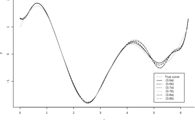
Figure 4.5 – Estimated curves for a sample with small variance.
0 1 2 3 4 5 6
−1
0
1
2
x
y
True curve (3.6a) (3.6b) (3.7a) (3.7b) (3.8a) (3.8b)
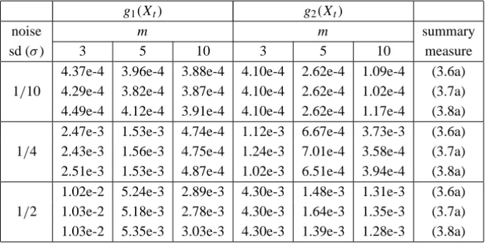
To see the performance of Algorithm 3.1, we run several simulations with different values of m, different variances for the functions given by (4.1) and (4.2). As expected, the larger the variance, the lower the quality of the estimation. On the other hand, we have provided consistent estimators (the bigger the sample size the better the estimate). Table 4.1 summarizes these results. All summary measures give approximately the same resulting curve. Measure (3.7a) gives better results for high variance or bigger sample size, while (3.8a) is better for all other cases, except one where (3.6a) is better. The occurrence of several identical results is caused by the simplicity of the curves and small sample size reducing the number of different solutions.
g1(Xt) g2(Xt)
noise m m summary
sd (σ) 3 5 10 3 5 10 measure
4.37e-4 3.96e-4 3.88e-4 4.10e-4 2.62e-4 1.09e-4 (3.6a) 1/10 4.29e-4 3.82e-4 3.87e-4 4.10e-4 2.62e-4 1.02e-4 (3.7a) 4.49e-4 4.12e-4 3.91e-4 4.10e-4 2.62e-4 1.17e-4 (3.8a) 2.47e-3 1.53e-3 4.74e-4 1.12e-3 6.67e-4 3.73e-3 (3.6a) 1/4 2.43e-3 1.56e-3 4.75e-4 1.24e-3 7.01e-4 3.58e-4 (3.7a) 2.51e-3 1.53e-3 4.87e-4 1.02e-3 6.51e-4 3.94e-4 (3.8a) 1.02e-2 5.24e-3 2.89e-3 4.30e-3 1.48e-3 1.31e-3 (3.6a) 1/2 1.03e-2 5.18e-3 2.78e-3 4.30e-3 1.64e-3 1.35e-3 (3.7a) 1.03e-2 5.35e-3 3.03e-3 4.30e-3 1.39e-3 1.28e-3 (3.8a)
Table 4.1 – MSE between the estimate and the true curve.
5 Registration
Registration techniques can be found in Ramsay and Li (1998) and Ramsay (2003). The implementation of these techniques are available in R and Matlab. The package fda in R language has two available techniques landmark and
continuous registration.
The landmark technique is appropriate when the curves to be registered
have prominent features like valleys and peaks. Suppose we have curves
g0,g1, . . . ,gm to be registered and they present Q of such properties at points
at ti,Q+1 of the i th curve are also considered and Q+2 properties are to be
used in computing the warping function h(t). This function h is such that the
registration of the curve gi(t)is given by
gi(h(ti q))=g0(t0q), for q =0, . . . ,Q+1. (5.1)
The goal is to make a time transformation such that the Q+2 properties are
aligned in time. In the R package, the user provides the placement of the Q properties for each curve which makes the process highly subject to error. For example, certain curves do not present one or more of the critical points or there is ambiguity where to place them. When there are too many curves and/or too many properties the marking is too tedious. However, Ramsay (2003) showed that automatic methods for mark identification can lead to serious mistakes.
The continuous registration method tries to solve these problems. It maximizes a measure of similarity among the curves,
F(h)=
Z b
a
[gi(h(t))−g0(t)]2 dt, (5.2)
where[a,b] is the observation interval. This measure takes into account the
whole curve and not only the critical points and it works well if h has good
properties such as smoothness. However, it fails if gi and g0 differs also in
range. This routine needs that the functions gi and g0 be given in functional
form which can be obtained using Fourier series or B splines, for example.
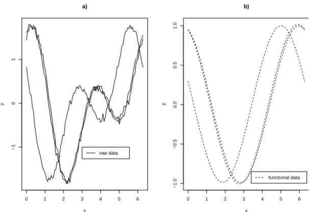
In Figure 5.7 we present an example where we simulated m=3 curves adding
a low variance noise and shifting it through an uniform random variable in the interval [0,2]. In this case, since the functions are periodic we used Fourier expansion with 6 terms. Figure 5.8 presents the registered curves. Observe that there is a noticeable difference between the structural mean and the true curve caused by the failure of the registration of two of the curves.
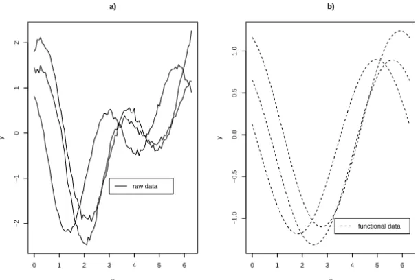
Consider another example where the curves have a range and phase variation. To obtain this effect we fixed the horizontal axis as a reference and defined as “bumps” the pieces of the true curve between two zeroes. Following, for each bump generate q2i q, i =1, . . . ,m,q =1, . . . ,Q (Q = number of bumps)
0 1 2 3 4 5 6
−1
0
1
a)
x
y
raw data
0 1 2 3 4 5 6
−1.0
−0.5
0.0
0.5
1.0
b)
x
y
functional data
Figure 5.7 – A simple shifting case: a. Simulated curves; b. Curves obtained using
create.fourier.basis().
0 1 2 3 4 5 6
−1.5
−1.0
−0.5
0.0
0.5
1.0
1.5
x
y
registered data structural mean true curve
Figure 5.8 – A simple shifting case – Registered curves usingregisterfd().
for the raw data and the functional data using Fourier transformation. Figure
5.10 presents the result of registration done by R routineregisterfd(). As
0 1 2 3 4 5 6
−2
−1
0
1
2
a)
x
y
raw data
0 1 2 3 4 5 6
−1.0
−0.5
0.0
0.5
1.0
b)
x
y
functional data
Figure 5.9 – A complex shifting case: a. Simulated curves; b. Curves obtained using
create.fourier.basis().
0 1 2 3 4 5 6
−2
−1
0
1
2
x
y
registered data structural mean true curve
Figure 5.10 – A complex shifting case – Registered curves usingregisterfd().
To overcome this problem we propose a modification in the continuous regis-tration procedure. Based on (5.2) we try to minimize the cumulative difference
diffe-rent range we normalize them using
gi∗= gi −min gi max gi −min gi
. (5.3)
From this point on, we can use an idea similar to Ramsay (2003) which suggests to substitute each curve by itsν-derivative, and our goal is to minimize
˜
1i =arg min
1i
Z b
a
Dνgi∗(t+1i)−g0∗(t) 2
dt (5.4)
for each curve i , i = 1, . . . ,m. In this work we decide to use ν = 0. The
procedure is described by Algorithm 5.1. We used the sample points as a grid to find1˜i.
Algorithm 5.1
1. Use Algorithm 3.1 to obtain the functional representation of each curve.
2. Normalize each curve using Equation (5.3).
3. Obtain1˜i for each of the normalized curves.
4. Shift the non-normalized curves taking gi(t+ ˜1i).
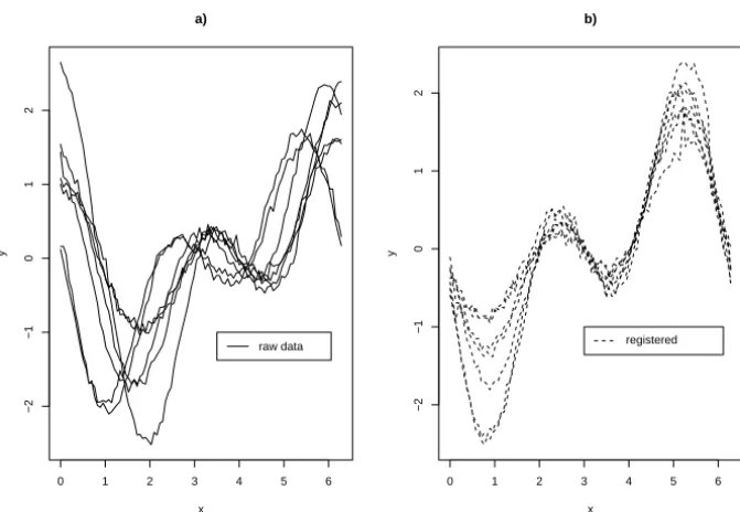
Figure 5.11 presents a sample of m =7 curves having phase and range
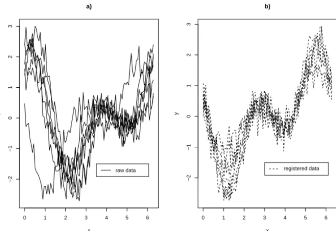
vari-ation plus a low variance noise. Figure 5.12 shows the registered curves after the application of Algorithm 5.1. All estimates using (3.6a), (3.7a) and (3.8a) were very similar and presented small MSE. Afterward we amplified the noise by taking a variance 25 times bigger, see Figure 5.13. Figure 5.12 shows the registered curves after the application of Algorithm 5.1. It seems that a good registration of the curves was achieved.
0 1 2 3 4 5 6
−2
−1
0
1
2
a)
x
y
raw data
0 1 2 3 4 5 6
−2
−1
0
1
2
b)
x
y
registered
Figure 5.11 – A complex shifting case: a. Simulated curves; b. Curves obtained using
Algorithm 5.1.
0 1 2 3 4 5 6
−2
−1
0
1
2
x
y
true curve (3.6a) (3.7a) (3.8a)
0 1 2 3 4 5 6
−2
−1
0
1
2
3
a)
x
y
raw data
0 1 2 3 4 5 6
−2
−1
0
1
2
3
b)
x
y
registered data
Figure 5.13 – A complex shifting case: a. Simulated curves plus a large variance noise;
b. Curves registered using Algorithm 5.1.
REFERENCES
[1] G. Celeux and J. Diebolt, A stochastic approximation type EM algorithm for the mixture problem, Stochastics Rep., 41 (1-2) (1992), 119–134.
[2] G. Celeux, D. Chauveau and J. Diebolt, Stochastic versions of the EM algorithm: an experi-mental study in the mixture case, J. of Statist. Comput. Simul., 55 (1996), 287–314. [3] D. Chauveau, A stochastic EM algorithm for mixtures with censored data, J. Statist. Plann.
Inference, 46 (1) (1995), 1–25.
[4] A.P. Dempster, N.M. Laird and D.B. Rubin, Maximum likelihood from incomplete data via the EM algorithm, J. Roy. Statist. Soc. Ser. B, 39 (1) (1977), 1–38. With discussion. [5] R. Dias and D. Gamerman, A Bayesian approach to hybrid splines non-parametric regression,
Journal of Statistical Computation and Simulation, 72 (4) (2002), 285–297.
[6] J. Diebolt and G. Celeux, Asymptotic properties of a stochastic EM algorithm for estimating mixing proportions, Comm. Statist. Stochastic Models, 9 (4) (1993), 599–613.
[7] J.O. Ramsay, Matlab, r and s-plus functions for Functional Data Analysis, ftp://ego.psych.
mcgill.ca/pub/ramsay/FDAfuns, (2003).
[9] J.O. Ramsay and B.W. Silverman, Applied functional data analysis, Springer Series in Sta-tistics, Springer-Verlag, New York. Methods and case studies, (2002).