ISSN 0101-8205 www.scielo.br/cam
Axiomatization of the index of pointedness
for closed convex cones
ALFREDO IUSEM1 and ALBERTO SEEGER2
1Instituto de Matemática Pura e Aplicada
Estrada Dona Castorina 110, Jardim Botânico, Rio de Janeiro, Brazil 2Univ. of Avignon, Department of Mathematics
33, rue Louis Pasteur, 84000 Avignon, France E-mails: [email protected] / [email protected]
Abstract. LetC(H)denote the class of closed convex cones in a Hilbert spaceH. One possible way of measuring the degree of pointedness of a coneKis by evaluating the distance fromKto the set of all nonpointed cones. This approach has been explored in detail in a previous work of ours. We now go beyond this particular choice and set up an axiomatic background for addressing this issue. We define an index of pointedness overHas being a function f:C(H)→Rsatisfying a certain number of axioms. The number f(K)is intended, of course, to measure the degree of pointedness of the coneK. Although several important examples are discussed to illustrate the theory in action, the emphasis of this work lies in the general properties that can be derived directly from the axiomatic model.
Mathematical subject classification: 47L07, 52A20. Key words:pointed cone, solid cone, index of pointedness, duality.
1 Introduction
LetH be a real Hilbert space with inner producth∙,∙iand associated normk∙k. For the sake of clarity in the exposition, we always assume that
2≤dim H <∞.
Some of our results can be extended to an infinite dimensional setting, but at the price of a more obscure presentation. The leading role in our discussion is not played by the linear spaceH, but rather by the metric space
C(H)= {K ⊂ H: K is a nonempty closed convex cone}.
The metric considered inC(H)is the usual one, namely
δ(K1,K2)= sup
kzk ≤1|
dist[z,K1] −dist[z,K2]|, (1)
where the notation dist[z,K]refers to the distance fromztoK.
The purpose of this work is to elaborate an axiomatic model for dealing with the concept of pointedness. Recall thatK ∈C(H)is calledpointedifK∩−K = {0}.
In other words, a cone is pointed if, and only if, it contains no line. Pointedness is a “qualitative” property that has far-reaching consequences. There is no shortage of beautiful theorems in which pointedness plays a prominent role.
Imagine that you have a pointed cone defined in terms of a certain parameter. What happens with the pointedness of the cone if the parameter changes slightly? How much you need to perturb the cone in order to destroy its pointedness? Robustness of a given property is one of the commonest issues addressed by scientists and engineers alike. In the present work we wish to “quantify” the degree of pointedness of a cone. This topic was already addressed in our previous paper [5], but now the orientation is entirely different. Instead of working with a particular measure of pointedness, we set up an axiomatic model from which a more general theory can be developed.
Enough has been said about our motivation. As far as notation is concerned, everything is more or less standard:
BH = {x ∈ H: kxk ≤1} (closed unit ball inH)
SH = {x ∈ H: kxk =1} (unit sphere in H)
K+= {y∈ H: hy,xi ≥0 ∀x ∈ K (dual cone ofK)
diam()=sup{ku−vk :u, v∈} (diameter of)
2 The index of pointedness: an axiomatic formulation
If f(K)is intended to measure the degree of pointedness of a coneK ∈C(H),
which are the properties that f should satisfy?
• Primo, it is natural to require that f discriminate between the pointed case and the nonpointed one, for instance, f(K) >0 if K is pointed, and
f(K)=0 if K is not pointed.
• Secundo, there is no doubt that a rayR+e= {μe:μ∈R+}(e6=0) is an
extremely pointed object, so it should have the highest possible degree of pointedness. As far as the zero-coneOH = {0}is concerned, there are two acceptable strategies: either we take it away from the discussion, or we treat it as a “degenerate” ray (corresponding toe=0). If the latter strategy is adopted, the degree of pointedness ofOH should also be maximal.
• Tertio, changing the orientation of a ray, or, more generally, changing the orientation of a cone, should not affect its degree of pointedness.
This is the bare minimum. To this one could add an extra condition: the degree of pointedness of a cone should diminish if the cone gets bigger. And last, but not the least, if two cones are close to each other, then their corresponding degrees of pointedness should not be too different.
We are now ready to state a formal definition The notation Isom(H)refers to the space of linear isometries onH (i.e., linear operatorsU: H → H such that
kU xk = kxk ∀x ∈ H).
Definition 2.1. An index of pointedness on H is a continuous function
f:C(H)→Rsatisfying the following axioms:
(A1) minimal pointedness: f(K)=0 if and only ifK is not pointed;
(A2) maximal pointedness: f(K) = 1 if and only if K is either a ray or the zero-cone;
(A3) invariance property: f(U(K))= f(K) ∀ K ∈C(H), ∀U ∈Isom(H);
By convention, the minimal degree of pointedness has been fixed at level 0, and the maximal one at level 1. We could work with any other scale and the whole theory would remain essentially the same.
Proposition 2.2. Let f be an index of pointedness on H. Then,
{f(K): K ∈C(H)} = [0,1]. (2)
Proof. The monotonicity axiom allows us to write
OH ⊂K ⊂H =⇒ f(H)≤ f(K)≤ f(OH).
Since f(H)=0 and f(OH)=1, one obtains{f(K): K ∈C(H)} ⊂ [0,1]. To
prove the reverse inclusion, consider an arbitrary unit vectore∈ Hand define
R(t)= {x ∈ H:tkxk ≤ he,xi} ∀t∈ [0,1]. (3)
A matter of computation yields the estimate
δ(R(t),R(s))= |tp1−s2
−sp1−t2
| ∀t,s ∈ [0,1].
Hence,R: [0,1] →C(H)is a continuous path joining the half-space
R(0)= {x ∈ H: he,xi ≥0}
to the ray R(1) = R+e. As a consequence, the continuous functiont ∈ [0,1]
7→ f(R(t))takes all the intermediate values between f(R(0))=0 and f(R(1))
= 1.
Remark. If the monotonicity requirement (A4) in Definition 2.1 is replaced by
(A4)′ 0≤ f(K)≤1 ∀K ∈C(H),
then one gets a weakened set of axioms. A continuous function f:C(H)→R
The monotonicity requirement(A4)adds some substance to the discussion, but it is not really the fundamental ingredient.
Definition 2.1 is now going to be scrutinized in detail. As often happens, a good set of axioms leads eventually to a powerful theory which allows people to go far beyond their original expectations. To start with, observe that the class
χ (H)= {f:C(H)→R: f is an index of pointedness on H}
is stable with respect to a number of averaging operations:
Proposition 2.3. If f1,∙ ∙ ∙, fm are indices of pointedness on H , then any of the following choices corresponds to a new index of pointedness on H :
(a) lower envelope: f(K)=min{f1(K),∙ ∙ ∙, fm(K)};
(b) upper envelope: f(K)=max{f1(K),∙ ∙ ∙ , fm(K)};
(c) arithmetic average: f(K)= f1(K)+∙∙∙+fm(K)
m ;
(d) geometric average: f(K)=[f1(K)∙ ∙ ∙ fm(K)]1/m ;
(e) harmonic average: f(K)=
n
[f1(K)]−1+∙∙∙+[fm(K)]−1
m
o−1
;
(f) log-sigma average: f(K)=loghef1(K)+∙∙∙+efm(K)
m
i
.
Proof. Everything can be checked quite easily, so the details are omitted.
One might also think of more sophisticate ways of forming averages, but such a discussion is only of marginal interest. What is perhaps more important to clarify is whether two given members ofχ (H)can be linked together through a simple scaling operation:
f2∼ f1 ⇐⇒ ∃γ ∈Ŵ such that f2=γ ◦ f1, (4)
where the familyŴof “scaling functions” is given by
Of course, eachγ ∈ Ŵis necessarily continuous and satisfies γ (0) = 0 and
γ (1)=1. One can easily check that (4) is an equivalence relation overχ (H)(i.e., it is reflexive, symmetric, and transitive). Observe that the indices of pointedness
p
f(∙), [f(∙)]2, sinhπ 2 f(∙)
i
, log[1+ f(∙)]
log2 , ∙ ∙ ∙
are all equivalent to the index of pointedness f in the sense that they belong to the same equivalence class, namely, the class of f.
Most of the interesting indices of pointedness are not just continuous in the ordinary sense, but also Lipschitz continuous. Recall that a function f:C(H)→ Ris said to be Lipschitz continuous if the number
lip(f)= sup
K16=K2
|f(K1)− f(K2)| δ(K1,K2)
is finite. The function f:C(H)→Ris declarednonexpansiveif
|f(K1)− f(K2)| ≤ δ(K1,K2) ∀K1,K2∈C(H).
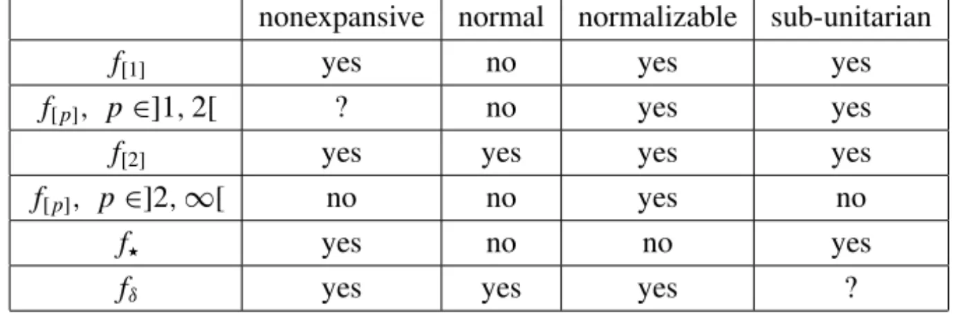
3 Three fundamental examples
Among the different members ofχ (H), some deserve a special mention due to their additional topological properties, or simply because they have an interesting geometric interpretation.
3.1 The basic approach
The term “basic” must be understood in a literal sense. Recall that a set⊂ H
is called abasefor the cone K ∈C(H)if
0∈/ and K =R+. (5)
The last condition in (5) is expressed by saying thatgenerates the coneK. As an example of base for K 6= OH, one may think of the compact set K ∩SH. By taking the convex hull ofK∩SH, one gets a convex compact set generating
caught in co(K∩SH). As part of the folklore of the theory of convex cones, one knows that
K is pointed ⇐⇒ 0∈/co(K ∩SH). (6)
This observation leads us to introduce the number
f⋆(K)=dist[0,co(K ∩SH)] (7)
as a candidate for measuring the degree of pointedness ofK 6= OH. As far as the zero-cone is concerned, we adopt the convention f⋆(OH)=1. The lemma
stated below provides a “dual” characterization of (7). The notation
x ∈ H 7→9∗(x)=sup
u∈h
u,xi
refers to the support function of⊂ H. We assume that the reader is familiar with the main properties of support functions (see, for instance, [4] or [8]). For the sake of convenience, we introduce also the notation
C0(H)=C(H)\{OH}.
Lemma 3.1. For any K ∈C0(H), one can write
f⋆(K)= sup
kxk≤1−
9∗K∩S
H(x). (8)
Proof. Formula (8) is obtained by applying a standard minimax argument. Observe that
f⋆(K)= inf
u∈co(K∩SH)xsup∈B
H
hu,xi.
Since co(K ∩SH)andBH are convex compact sets, von Neumann’s minimax theorem allows us to exchange the order of inf and sup. This produces
f⋆(K) = sup
x∈BH inf
u∈co(K∩SH)h
u,xi
= sup
kxk≤1−
9co∗(K∩S
H)(−x)
= sup
kxk≤1−
9co∗(K∩S
H)(x).
The convex hull operation can be dropped from the last term, getting in this way
Before proving that f⋆ is an index of pointedness, it is helpful to recall some
known properties of the Pompeiu-Hausdorff metric
haus[C1,C2] =max{sup
a∈C1
dist[a,C2],sup
b∈C2
dist[b,C1]}.
Lemma 3.2. If C1and C2are two nonempty compact sets in H , then
haus[C1,C2] ≥haus[co(C1),co(C2)] = sup
kxk≤1
9C∗
1(x)−9
∗ C2(x)
. (9)
Proof. The support function characterization of haus[co(C1),co(C2)] is well known in the convex analysis community (cf. Theorem 2.18 in Castaing and Valadier [3], or Corollary 3.2.8 in Beer [1]). The inequality in (9) can be found, for instance, in the book by Kisielewicz [7]. Such inequality is almost trivial due
to inclusion.
We now are ready to state:
Proposition 3.3. The function f⋆is a nonexpansive index of pointedness on H .
Proof. Axiom(A1)is a consequence of (6). Since the functionk∙k2is strictly convex, the equality dist[0,co(K∩SH)] =1 occurs if and only if the setK∩SH
is a singleton. This takes care of(A2). To check the invariance property(A3), just notice that
co[U(K)∩SH] =co[U(K ∩SH)] =U[co(K ∩SH)] ∀U ∈Isom(H).
Monotonicity of f⋆is obvious. For proving nonexpansiveness, we rely on
Lem-mas 3.1 and 3.2. First of all, it must be observed thatδcan be characterized in terms of the Pompeiu-Hausdorff metric, to wit
δ(K1,K2)=haus[K1∩BH,K2∩BH] ∀ K1,K2∈C(H).
To avoid trivialities, suppose that both cones K1,K2 are inC0(H). In such a
case, one can write
and, with the help of Lemma 3.2, one gets
−9∗K
1∩SH(x)≤ −9
∗
K2∩SH(x)+δ(K1,K2) ∀x ∈ BH.
By taking the supremum overBH and applying Lemma 3.1, one obtains
f⋆(K1)≤ f⋆(K2)+δ(K1,K2).
It suffices now to exchange the roles ofK1andK2to complete the proof.
3.2 The hemi-diametral approach
It is based on the evaluation of the number
r(K)= 1
2 diam(K ∩SH),
which corresponds to half the diameter of K ∩SH. Observe that the mapping
K 7→r(K)ranges from 0 (whenK is a ray) to 1 (whenK is nonpointed). Since
r has not the right monotonicity, we suggest considering instead
f[1](K)=1−r(K).
In fact, one can also consider the more general expression
f[p](K)=
1− [r(K)]p1/p, (10)
withp∈ [1,∞[being chosen arbitrarily. The casep =2 is of special relevance as we shall see in due course. The term (10) makes sense only ifK 6= OH, so, by convention, one sets f[p](OH)=1. As shown in the next lemma, the functionr
has a fairly good continuity behavior.
Lemma 3.4. For any K1,K2∈C0(H), one has the Lipschitz estimate
Proof. This result is probably known. In order to prove (11), we start by ob-taining an alternative characterization of the diameter function. For a nonempty bounded set⊂H, one can write
diam()= sup
u,v∈
sup
x∈BH
hx,u−vi = sup
x∈BH sup
u,v∈{h
x,ui + hx,−vi},
producing in this way
diam()= sup
x∈BH
{9∗(x)+9−∗(x)}.
We will apply this general formula to the particular choices= K1∩SH and
=K2∩SH. By Lemma 3.2, we know already that
9K∗
1∩SH(x)≤9
∗
K2∩SH(x)+δ(K1,K2) ∀x ∈ BH, as well as,
9−∗(K
1∩SH)(x)≤9
∗
−(K2∩SH)(x)+δ(−K1,−K2) ∀x ∈ BH. Summing up and observing thatδ(−K1,−K2)=δ(K1,K2), one gets
9∗K
1∩SH(x)+9
∗
−(K1∩SH)(x) ≤ 9
∗
K2∩SH(x)+9
∗
−(K2∩SH)(x)
+2δ(K1,K2) ∀x ∈ BH.
To complete the proof, we just need to take the supremum with respect
to x ∈ BH.
Without further ado, we state:
Proposition 3.5. For each p ∈ [1,∞[, the function f[p] is an index of poin-tedness on H .
Proof. The diameter ofK∩SHequals 2 if and only ifKcontains two opposite unit vectors. The set K ∩SH is a singleton if and only if K is a ray. These statements take care of Axioms (A1) and(A2), respectively. The invariance property(A3)follows from
diam[U(K)∩SH] =diam[U(K∩SH)] =diam[K∩SH] ∀U ∈Isom(H).
Monotonicity of f[p] is obvious. Lemma 3.4 yields the continuity of K →
diam(K ∩SH)as function defined over metric subspaceC0(H). This fact
Proposition 3.6. For any p,q ∈ [1,∞[, the indices f[p]and f[q]are equiva-lent.
Proof. For passing from f[p]to f[q], consider the scaling function t ∈ [0,1] 7→γ (t)=1−(1−tp)q/p1/q.
It is a mere routine to check thatγ ∈Ŵ.
As mentioned before, the choice p = 2 is of special relevance. A simple computation shows that
f[2](K)=
p
1− [r(K)]2 (12)
admits the equivalent characterization
f[2](K)=
r
1+cosθmax(K)
2 =cos
θmax(K)
2
, (13)
whereθmax(K)denotes the largest angle that can be formed by picking up two
unit vectors inK, that is to say
θmax(K)= sup u,v∈K∩SH
arccoshu, vi.
Due to the formula (13), we refer to f[2](K)as theangular index of pointedness
of K (we reserve the term “angular” for the index f[2], but is is clear from
Proposition 3.6 that any hemi-diametral index f[p]can be expressed in terms of
the functionθmax).
The equivalence between (12) and (13) can be proven in a rather easy way by exploiting the general identity
ku−vk2=2(1− hu, vi) ∀u, v∈ SH.
Below we provide two additional characterizations of the function f[2]. Recall
that thegapbetween two nonempty sets A,B ⊂H is defined as the number
gap[A,B] = inf
a∈A,b∈Bka−bk.
Lemma 3.7. For any K ∈C0(H), one has
f[2](K)=
1
2 gap[K∩SH,−K∩SH], (14)
and also
f[2](K)= inf
kzk=1 max{dist[z,K], dist[−z,K]}, (15) Proof. Formula (14) is easier to prove. By definition of a gap, one has
gap[K∩SH,−K ∩SH] = inf
u∈K∩SH,w∈−K∩SHk
u−wk = inf
u,v∈K∩SHk
u+vk.
By working out the last expression, one arrives at
gap[K ∩SH,−K ∩SH] = inf
u,v∈K∩SH 2
r
1+ hu, vi
2 =2 f[2](K). Formula (15) is proven in our work [6]. The proof, which is quite long and technical, doesn’t deserve to be reproduced here. Observe, incidentally, that (15) applies also to the zero cone, the convention f[2](OH)=1 being in force.
Remark. As done in [6], it is interesting to observe that (
∀K ∈C0(H), there is a unit vectorz ∈ H
such that f[2](K)=dist[z,K] =dist[−z,K].
When K is not a ray, such a vectorzcan be constructed, for instance, by norma-lizingu−v, withu, v∈ K ∩SH satisfyingku−vk =diam(K∩SH).
We now return to the analysis of the family {f[p]: p ∈ [1,∞[} of
hemi-diametral indices. As shown in the next theorem, nonexpansiveness can be obtained only for special choices ofp. Before stating such a result, a preliminary lemma is in order. Observe that f[p]admits the representation
f[p](K)=ϕp(r(K)) ∀ K ∈C0(H), (16)
withϕp: [0,1] → [0,1]being defined byϕp(τ ) = [1−τp]1/p. Formula (16)
Lemma 3.8. Let p ∈]1,2[. Then, there exist τp ∈]0,1[ and a positive constant Lpsuch that
(a) |ϕp(t)−ϕp(s)| ≤Lp |t−s| ∀t,s ∈ [0, τp];
(b) |ϕp(t)−ϕp(s)| ≤ |ϕ2(t)−ϕ2(s)| ∀t,s ∈ [τp,1];
(c) |ϕp(t)−ϕp(s)| ≤ |ϕ2(t)−ϕ2(s)| +Lp|t−s| ∀t,s ∈ [0,1]. Proof. For proving the part (a), observe that the derivative
ϕ′p(τ )= −
τ (1−τp)1/p
p−1
is well defined over[0, τp], and
Lp = sup
τ∈[0,τp]
|ϕ′p(τ )|<∞.
The above remark applies to any choice ofτp ∈]0,1[. For proving the part (b),
we takeτpso that
ϕ′p(τ )≥ϕ2′(τ ) ∀τ ∈ [τp,1[. (17)
To check that such aτpexists, we write (17) in the form
τ (1−τp)1/p
p−1
≤ √ τ
1−τ2 ,
or, what is equivalent,
τ4−2p ≥ 1−τ
2
(1−τp)2(p−1)/p . (18)
Obviously, the left-hand side of (18) goes to 1 asτ →1−, while an application of l’Hôspital’s rule establishes that the right-hand side goes to 0 as τ → 1−.
Thus the inequality in (18) is valid for τ close enough to 1. Once (17) has been established for a suitableτp, one completes the proof of (b) by using an
difficult case in whichtandsare not on the same side with respect toτp. Take
for instance 0≤s < τp<t <1. Observe that
|ϕp(t)−ϕp(s)| = − [ϕp(t)−ϕp(s)]
= − Z t
s
ϕ′p(τ )dτ
= Z τp
s −
ϕ′p(τ )dτ +
Z t
τp
−ϕ′p(τ )dτ.
But Z τ
p
s −
ϕ′p(τ )dτ ≤ Lp(τp−s)≤ Lp |t−s|,
and
Z t
τp
−ϕ′p(τ )dτ ≤
Z t
τp
−ϕ2′(τ )dτ ≤ −[ϕ2(t)−ϕ2(τp)] ≤ |ϕ2(t)−ϕ2(s)|.
The proof of the lemma is thus complete.
Theorem 3.9. The following statements are true:
(a) the indices f[1]and f[2]are nonexpansive;
(b) for any p∈]1,2[, the index f[p]is Lipschitz continuous;
(c) for any p>2, the index f[p]is not Lipschitz continuous.
Proof.
• Part (a). Nonexpansiveness of f[1]is a direct consequence of Lemma 3.4.
Nonexpansiveness of f[2] follows from the characterization (15) and the
general inequality
dist[z,K1] ≤dist[z,K2] +δ(K1,K2) ∀z ∈SH, ∀K1,K2∈C(H).
• Part (b). To handle the casep∈]1,2[, we exploit Lemma 3.8 and the repre-sentation formula (16). Consider two arbitrary conesK1,K2∈C0(H). If
r(K1)andr(K2)fall both in the interval[0, τp], then Lemma 3.7(a) yields
Ifr(K1)andr(K2)fall both in the interval[τp,1], then we use Lemma
3.8(b) to obtain
|f[p](K2)− f[p](K1)| ≤ |f[2](K2)− f[2](K1)| ≤δ(K2,K1).
Ifr(K1)andr(K2)are not in the same side with respect toτp, then Lemma
3.8(c) does the job. One gets in this case
|f[p](K2)− f[p](K1)| ≤ |f[2](K2)− f[2](K1)| +Lp|r(K2)−r(K1)| ≤ (1+Lp) δ(K2,K1).
• Part (c). To handle the case p >2, consider the cone R(t)given by (3). As a matter of computation, one gets
f[p](R(t))=
h
1−p1−t2pi 1/p
∀t∈ [0,1],
and, therefore,
lip(f[p]) ≥ |
f[p](R(t))− f[p](R(0))|
δ(R(t),R(0))
= 1t h
1−p1−t2pi1/p
(19)
for anyt ∈]0,1[. Observe that the term on the right-hand side of (19) goes
to∞ast→0+.
3.3 The metric approach
We cannot avoid mentioning the function fδ:C(H)→ [0,1]defined by
fδ(K)= inf
Q∈M(H)
δ(Q,K). (20)
The number fδ(K)represents the distance fromK to the set
M(H)= {Q∈C(H): Qis not pointed}.
SinceM(H)is a compact set in the metric space(C(H), δ), the infimum in (20) is actually attained. In our work [5], we refer to the number fδ(K)as theradius
of pointednessofK. The reason for this name is that
corresponds to the radius of the largest ball
Ur(K)= {Q ∈C(H):δ(Q,K) <r}
centered atK and contained in the setP(H)=C(H)\M(H)of pointed cones.
Proposition 3.10. The function fδ is a nonexpansive pre-index of pointedness
on H .
Proof. See the reference [5].
Proposition 3.11. Among all the nonexpansive pre-indices of pointedness on H, fδ is the largest one (in the pointwise sense).
Proof. Take an arbitraryK ∈C(H). For any nonexpansive function f:C(H)
→R, one can write
f(K)≤ f(Q)+δ(Q,K) ∀ Q ∈C(H),
and, in particular,
f(K)≤ inf
Q∈M(H){f
(Q)+δ(Q,K)}.
If f vanishes overM(H), the above inequality reduces to f(K)≤ fδ(K).
It is not clear whether fδ satisfies the monotonicity requirement(A4). Partial
evidence leads us to conjecture that fδis indeed monotone, but we are not yet in
a position of giving a definite answer to this delicate issue.
4 Basic index versus angular index
Both indices share many properties in common, but they do behave differently with respect to dimensional issues. To start with, we state:
Proof. TakeK 6= {0}and write
f⋆(K) = inf
x∈co(K∩SH) k
xk
≤ inf
u,v∈K∩SH
u+v
2 = inf
u,v∈K∩SH r
1+ hu, vi
2 = f[2](K).
This proves the announced inequality.
The above proof hides, in fact, a general result:
Lemma 4.2. If K ∈ C(H) contains m mutually obtuse unit vectors, then f⋆(K)≤1/√m.
Proof. According to the hypothesis, one can findmunit vectorsa1,∙ ∙ ∙ ,am in
K such thathai,aji ≤0 ∀i 6= j. Hence,
[f⋆(K)]2 = inf
x∈co(K∩SH) k
xk2≤
a1+ ∙ ∙ ∙ +am m 2 = 1 m2 m X
i=1
kaik2+2X
i<j
hai,aji
.
Since the ai’s have unit length and are mutually obtuse, one gets [f⋆(K)]2
≤1/m.
With the help of Lemma 4.2 one can easily show that f⋆ 6= f[2], that is to say, f⋆(K) < f[2](K)for someK ∈C(H).
Example 4.3. Take H = Rn with n ≥ 3. Clearly, θmax(Rn+) = π/2 and f[2](Rn+)=1/
√
2. On the other hand, the positive orthantRn
+is a closed convex
cone containingnmutually orthogonal unit vectors. So,
f⋆(Rn+) ≤ 1/
√
n ≤ 1/√3 < f[2](Rn+).
The exact value of f⋆(Rn+)will be given in Proposition 4.9. As suggested by
dimension: the degree of pointedness of the corresponding positive orthant is almost zero. This “strange” behavior of f⋆ becomes even worse in an
infinite-dimensional setting: f⋆is no longer an index of pointedness!
Example 4.4. In the Hilbert spaceH =ℓ2of square summable real sequences, consider the pointed cone
ℓ2+= {x ∈ℓ2:xk ≥0 ∀k ∈N},
and the canonical vectorsa1=(1,0,0,∙ ∙ ∙), a2=(0,1,0,∙ ∙ ∙), . . . Since the firstncanonical vectors lie inℓ2+and are mutually orthogonal, it follows that
f⋆(ℓ2+)≤1/
√ n.
But this argument applies to an arbitraryn, so f⋆(ℓ2+) =0. In other words, f⋆
does not satisfy the axiom (A1). This fact should not be too surprising after all: one knows that the characterization (6) of pointedness holds only if the underlying space is finite dimensional.
The next proposition has to do with the particular case of a finitely generated cone, that is to say, a cone expressible as
K = {μ1g1+ ∙ ∙ ∙ +μmgm:μ∈Rm+}. (21)
Without loss of generality one may assume that the generatorsg1,∙ ∙ ∙ ,gm ∈Rn
are vectors of unit length. An upper bound for f⋆(K) is obtained easily by
minimizing a convex quadratic form over the elementary simplex
6m = {μ∈Rm+:μ1+ ∙ ∙ ∙ +μm =1}.
Proposition 4.5. Let K ⊂ Rn be the finitely generated cone given by (21). Denote by G the n×m matrix whose columns are the generators g1,∙ ∙ ∙,gm ∈ SRn. Then,
[f⋆(K)]2 ≤ inf μ∈6mh
Proof. It is enough to observe that f⋆(K)≤ kGμkfor everyμ∈6m.
One of the reasons for introducing the index f⋆is that its computational cost
is not too high. As indicated in the proof of Lemma 3.1, one has
f⋆(K)= sup
kxk≤1
ρK(x), (22)
with
ρK(x)= inf u∈K∩SHh
u,xi. (23)
Solving the inner minimization problem (23) amounts to finding a unit vector in
Kwhich forms the largest angle with respect to the givenx. The best choice for
x is obtained by solving the outer maximization problem (22).
Definition 4.6. AcentroidofK ∈C0(H)is a maximizer ofρK over BH, that
is to say, a vector in
ctr(K)= {x ∈ BH:ρK(x)= f⋆(K)}.
SinceρK: H →Ris a concave function, the set ctr(K)is nonempty compact
and convex. This set turns out to be a singleton if the coneK is pointed:
Proposition 4.7. A pointed cone K ∈ C0(H) admits exactly one centroid.
Moreover, the centroid lies in K∩SH.
Proof. Consider first the case of an arbitraryK ∈C0(H), be it pointed or not.
We claim that
x0∈ctr(K) ⇐⇒
(
there is a vectory ∈ N[x0,BH]such that
y ∈co(K ∩SH) and hy,x0i =ρK(x0),
(24)
where
N[x0,BH] =
(
{0} if kx0k<1,
R+x0 if kx0k =1
corresponds to the normal cone to BH at x0. Observe thatx0 ∈ ctr(K) if and only ifx0minimizes−ρKoverBH. Since we are dealing with a convex
and sufficient (cf. Theorem 27.4 in [8]). So,
ctr(K)= {x0∈ H:0∈∂(−ρK)(x0)+N[x0,BH]},
with∂ denoting the subdifferential operator in the sense of convex analysis. For obtaining (24), it is enough to observe that
−∂(−ρK)(x0) = ∂9∗K∩SH(−x0)
= {y∈ H: y∈co(K ∩SH) andhy,x0i =ρK(x0)},
the last equality being a consequence of a general calculus rule for computing the subdifferential of a support function (cf. Corollary 23.5.3 in [8]). Consider now the particular case in whichK is pointed. According to (24), the inequality
kx0k <1 must be ruled out because 0 ∈/ co(K ∩SH). Hence, the centroids of
K lie necessarily inSH. By writing
y =βx0 with β ∈]0,1],
one sees thatx0 =β−1y
∈ K. Summarizing, we have proven that ctr(K)is a nonempty convex set contained inK ∩SH. This implies, of course, that ctr(K)
contains exactly one element.
As shown by the proof of Proposition 4.7, the centroid of a nonzero pointed coneK can be characterized as follows:
x0is the centroid of K ⇐⇒
kx0k =1, ρK(x0)∈]0,1],
and
ρK(x0)x0∈co(K∩SH).
(25)
For a revolution cone, for instance, the centroid corresponds to the so-called axis of revolution. In fact, one has:
Proposition 4.8. Consider a revolution cone K = {x ∈ H: kxkcosϑ ≤
he,xi}with axis of revolution e ∈ SH and angle of revolution ϑ ∈ [0, π/2[. Then,
Proof. Pick up an arbitraryb∈ SH such thathb,ei =0. Since
u=(cosϑ)e+(sinϑ)b and v=(cos ϑ )e−(sinϑ)b
belong toK ∩SH, one has
f⋆(K)≤ k(u+v)/2k = k(cosϑ )ek =cosϑ.
On the other hand,
f⋆(K)≥ρK(e)= inf x∈K∩SHh
e,xi = cosϑ.
Another instance where the centroid can be easily computed is that of a positive orthant:
Proposition 4.9. The centroid of the positive orthant Rn
+ is x0 = n−1/2(1,1,∙ ∙ ∙,1), and
f⋆(Rn+) = ρRn
+(x0) = 1/ √
n. (26)
Proof. Clearlykx0k =1. It is geometrically clear that the infimal-value
ρRn
+(x0)=u∈Rninf +,kuk=1
u1+ ∙ ∙ ∙ +un √n
is attained at any of the generators ofRn
+. This allows us to check the right-hand
side of (25), and obtain the formula (26).
We end this section by showing that the basic index is essentially different from the angular index.
Proposition 4.10. WhendimH ≥3, the indices f⋆and f[2]are not equivalent. Proof. LetH =Rn, withn
≥ 3. The positive orthantRn
+and the ice-cream
cone
3n= {x ∈Rn: [x12+ ∙ ∙ ∙ +x 2 n−1]
1/2 ≤ xn}
have both a maximal angle equal toπ/2. Thus,
f[2](3n)= f[2](Rn+)=1/ √
On the other hand,
f⋆(3n)=1/ √
2 but f⋆(Rn+)=1/
√
n<1/√2.
This rules out the possibility of finding a scaling function γ ∈ Ŵ such that
f⋆ =γ ◦ f[2].
5 Normalization
Starting with an arbitrary index of pointedness, one can construct a new one by using a simple scaling procedure. If we are lucky enough, we could find a suitable scaling function bringing our initial index to a sort of “normal” form. This raises the question of what must be understood by a normal index. There are different ways of answering this question, everything depending on what we have in mind when we speak about normalizing an index.
Recall that the index of a nonpointed cone has been fixed at the minimum level 0, whereas the index of a ray has been fixed at the maximum level 1. So, what about an intermediate situation? What kind a cone could be considered as a good compromise between a nonpointed cone and a ray? Which one should be the corresponding index of such a cone?
To answer to these questions, we arrange the cones according to their maximal angle. On the one hand side, the caseθmax(K)=0 occurs whenK is a ray, and,
on the other hand, the conditionθmax(K) = π indicates that K is not pointed.
An interesting intermediate situation isθmax(K) =π/2. One can easily check
that
θmax(K)=
π
2 ⇐⇒ K is acute and contains a pair of
orthogonal unit vectors.
(27)
That K ∈ C(H)isacute simply means thathu, vi ≥ 0, ∀ u, v ∈ K. A cone
K ∈C(H)as in (27) is said to beperpendicular. We are now ready to introduce the concept of normality.
Definition 5.1. One says that f ∈χ (H)isnormalif
If there is a scaling functionγ ∈Ŵsuch thatγ ◦ f is normal, then f is declared
normalizable.
In other words, an index of pointedness is normalizable if and only if it is constant over the class of perpendicular cones. By way of example, we mention that the basic index f⋆is not normalizable: as shown in the proof of Proposition
4.10, f⋆takes different values over the class of self-dual cones (which is contained
in the class of perpendicular cones). The angular index f[2]behaves much better
in this respect:
Proposition 5.2. For any K ∈C(H), one has:
(a) f[2](K)≥ √
2/2if and only if K is acute;
(b) f[2](K)≤ √
2/2if and only if K contains a pair of orthogonal unit vectors.
Hence, the index f[2]is normal.
Proof. It follows directly from the characterization (13).
Corollary 5.3. The pre-index fδis normal.
Proof. As shown in [6], the functions fδ and f[2] coincide over the class of
perpendicular cones. It suffices then to apply Proposition 5.2. We observe, incidentally, that fδand f[2]coincide over a larger class of cones, namely,those
having a maximal angle less than or equal to 120 degrees.
Proposition 5.2 can be extended in the following way:
Proposition 5.4. Suppose that the index f ∈ χ (H) is of the angular-type, meaning that
Proof. Consider anyθ ∈ [0, π]. If f is of the angular-type, then f is constant over the level set
{θmax=θ} = {K ∈C(H):θmax(K)=θ}.
In particular, f is constant over {θmax = π/2}, the class of perpendicular
cones.
Remark. Any index f[p]from the hemi-diametral family is of the angular-type,
so it is normalizable.
6 Dualization
Recall that a cone K ∈ C(H) is said to be solid if its topological interior is
nonempty. In a finite dimensional setting, solidity is a dual concept with respect to pointedness:
K is pointed ⇔ K+is solid. (29)
A simple proof of this equivalence can be found, for instance, in the book by Berman [2]. Inspired by (29), we dualize the concept of pointedness index in the following manner:
Definition 6.1. Anindex of solidityonHis a continuous functiong:C(H)→
Rsatisfying the following axioms:
(A1) minimal solidity: g(K)=0 if and only if K is not solid;
(A2) maximal solidity: g(K)=1 if and only ifK contains a halfspace;
(A3) invariance property: g(U(K))=g(K) ∀ K ∈C(H), ∀U ∈Isom(H);
(A4) upward monotonicity: K1⊂ K2 implies g(K1)≤g(K2).
of pointedness of its polar K+. This idea is stated properly in the following
proposition, where we use the notation
8:C(H)7→C(H)
K 7→8(K)=K+
to indicate the polarity mapping. A celebrated theorem by Walkup and Wets [9] asserts that8is an isometry over the metric space(C(H), δ), i.e.
δ(K1+,K2+)=δ(K1,K2) ∀ K1,K2∈C(H).
Proposition 6.2. The polarity mapping8:C(H)7→C(H)relates the concepts
introduced in Definitions2.1and6.1as follows:
(a) if f is an index of pointedness, then f ◦8is an index of solidity;
(b) if g is an index of solidity, then g◦8is an index of pointedness.
Proof. Everything is straightforward. It is a matter of exploiting the well
known properties of the mapping8.
As pointed out to us by Adrian Lewis (personal communication), a possible way of measuring the degree of solidity of a coneK is in terms of the expression
g⋆(K)=sup{r: kxk =1,r ≥0,x +r BH ⊂ K}. (30)
This corresponds to the radius of the largest ball contained inK and centered at a unit vector. One assumes, of course, that K 6= H, otherwise the convention
g⋆(H) =1 is in order. It turns out that (30) defines an index of solidity in the
sense of Definition 6.1:
Proposition 6.3. The function g⋆ given by (30) is a nonexpansive index of
solidity. In fact,
g⋆(K)= f⋆(K+) ∀K ∈C(H), (31)
Proof. Suppose thatK ∈C(H)is not the whole space. Write (30) in the form
g⋆(K)= sup
kxk=1
sup r≥0 x+r BH⊂K
r
and observe that
x+r BH ⊂K ⇐⇒ rkyk ≤ hx,yi ∀ y ∈ K+ ⇐⇒ r ≤ inf
kyk=1
y∈K+
hx,yi.
This proves that
g⋆(K)= sup
kxk=1
inf
kyk=1
y∈K+
hx,yi.
The above expression remains unchanged ifx ranges over the unit ballBH (and not just over the unit sphereSH). Also, no change occurs if the infimum is taken over convex hull ofK+∩SH(and not just overK+∩SH). As we did in Lemma 3.1, we apply von Neumann’s minimax theorem to conclude that
g⋆(K)= sup
x∈BH inf
y∈co(K+∩SH)
hx,yi = inf
y∈co(K+∩SH) sup
x∈BH
hx,yi = f⋆(K+).
The proof of (31) is thus complete. Propositions 3.3 and 6.2 do the rest of
the job.
Observe that the formula (31) can be written in the equivalent form
f⋆(K)=g⋆(K+) ∀K ∈C(H), (32)
that is to say, the basic index of pointedness of a cone K can be computed by evaluating the index of solidityg⋆atK+. For illustrating this general principle,
we examine next the particular case of a nondegenerate elliptic cone inRn×R.
Such term refers to a set of the form
E(A)= {(u,s)∈Rn×R:√utAu≤s},
with Abeing a positive definite symmetric matrix of ordern×n. The symbol
Proposition 6.4. Let A be a positive definite symmetric matrix of order n×n. Then,
f⋆(E(A))=
s
λmin(A)
1+λmin(A)
and g⋆(E(A))=
s 1 1+λmax(A)
,
with λmin(A) and λmax(A) denoting, respectively, the smallest and largest eigenvalue of A.
Proof. Due to the formula (32) and the general identity[E(A)]+ = E(A−1),
we need to evaluate only the termg⋆(E(A)). To do this, we look at the largest
ball centered atxˉ =(0,∙ ∙ ∙ ,0,1) ∈ Rn×Rand contained inE(A). For this
it suffices to find the closest point to xˉ in the boundary ofE(A): the distance
from such point toxˉ will be the radius of such largest ball. Since the boundary ofE(A)is given by
bd[E(A)] = {(u,s)∈Rn×R:√utAu =s},
we must solve the minimization problem
min utu+(s−1)2 with (u,s)∈Rn×R s.t. utAu−s2=0. (33) If(u,s)is a solution to (33), then there is a Lagrange multiplierλ∈Rsuch that
u−λAu=0, s−1+λs =0.
Notice that λis an eigenvalue of A−1, u is a corresponding eigenvector, and
s =(1+λ)−1. Clearly
(1+λ)−2=s2=utAu=λ−1utu, (s−1)2=
1 1+λ−1
2 =
λ
1+λ
2
,
from where one obtains
utu+(s−1)2= λ (1+λ)2 +
λ2
(1+λ)2 =
We conclude that the optimal valuer2of (33) is of the form(1
+λ−1)−1, with
λ >0 being an eigenvalue of A−1. One can easily see that the smallest value of r =(1+λ−1)−1/2
is obtained by choosingλ=λmin(A−1). One gets in this way the estimate g⋆(E(A))≥
1+ [λmin(A−1)]−1
−1/2
= [1+λmax(A)]−1/2.
But, on the other hand, one can also write
g⋆(E(A))≤g[2](E(A))= [1+λmax(A)]−1/2. (34)
The inequality in (34) follows from Propositions 4.1 and 6.3, while the equality
in (34) is a result established in [5].
In the next proposition we provide an expression for the index of solidity
g[p]which is obtained by dualizing the index of pointedness f[p].
Proposition 6.5. Let g[p]:C(H)→Rbe the function defined by the expression g[p](K)=
1− [m(K)]p1/p, (35)
with
m(K)= sup
kzk=1
min{dist[z,K], dist[−z,K]}.
Then, g[p]is an index of solidity. In fact,
g[p](K)= f[p](K+) ∀K ∈C(H). (36)
Proof. We need to prove the equality (36). The case K = H is trivial and therefore it is left aside. Consider then an arbitraryK 6= H. Proving (36) is, of course, the same as checking the equality
m(K)=r(K+). (37)
To do this, we exploit Lemma 3.7 and the well-known Pithagorean rule
withK−= −K+standing for the negative polar cone ofK. Indeed, one has
r2(K+) = 1− f[22](K+) = 1− f[22](K−)
= 1−
inf
kzk=1 max{dist[z,K
−], dist[−z,K−]}
2
= 1− inf
kzk=1 max{1−dist 2
[z,K], 1−dist2[−z,K]}.
A simple algebraic manipulation shows that the last term corresponds tom2(K).
The proof is then complete.
As far as the dualization of the pre-index of pointedness fδ is concerned, we
have shown in [5] the formula
gδ(K)= fδ(K+) ∀K ∈C(H),
withgδ being the distance function to the set of non-solid cones, that is to say,
gδ(K)=inf{δ(Q,K): Q∈C(H)non-solid}.
7 Interlude: a tale of maximal angles
Recall thatθmax(K)denotes the maximal angle that can be formed by picking up
two unit vectors inK. The symbolθmax(K+)is defined, of course, in a similar
way. The question we would like to answer in this section has a very strong geometric flavour:
(
is there any relationship between the maximal angles θmax(K) and θmax(K+)?
(38)
It would be very surprising if nobody has thought about this question before. Anyway, we have been unable to find a trace of this issue in the existing literature. Anwering (38) would enable us to establish a link between the angular index of a cone and the angular index of its dual. For convenience, we reformulate (38) in a seemingly different manner:
(
is there any relationship between the diameter of K ∩SH and the diameter of K+∩SH ?
Lemma 7.1. Assume that K ∈ C(H)is neither the zero-cone, nor the whole
space H . Then,
[diam(K ∩SH)]2+ [diam(K+∩SH)]2≥4. (39)
Proof. If bothK ∩SH andK+∩SH have a diameter greater than or equal to √
2, then the result holds trivially. We assume from now that this is not the case. Suppose, for instance, that diam(K ∩SH) < √2. Due to (12) and (13), this assumption entails
hu, vi>0 ∀u, v∈ K. (40)
If K is a ray, then diam(K ∩SH) = 0, diam(K+∩SH) = 2, and (39) holds. Assume thatK is not a ray, and takeu, v∈ K ∩SH such that diam(K ∩SH)=
ku−vk > 0. Let M = span{u, v} be the two-dimensional linear subspace spanned byuandv. Consider the vectors
y = pu− hu, viv
1− hu, vi2 , z=
v− hu, viu
p
1− hu, vi2.
By construction,y ∈ Mandz∈ Menjoy the following properties:
hy,ui ≥0, hz, vi ≥0,
hz,ui = hy, vi =0,
hy,zi = −hu, vi,
kyk = kzk =1.
Everything can be checked in a rather easy way. We will prove thaty,zbelong to
K+. To do this, it suffices to show thathy,xi ≥0,hz,xi ≥0 for allx ∈ K∩SH.
So, takex ∈ K ∩SH. We find the projection PM(x)ofx onto Mby solving a simple minimization problem in two variables. We get
PM(x)=λu+μv,
with coefficientsλ, μ∈Rgiven by
λ= hu,xi − hx, vihu, vi
1− hu, vi2 , μ=
hv,xi − hx,uihu, vi
We claim thatλ, μ≥0. By (40) we know thathx,ui,hx, vi ∈]0,1]andhu, vi ∈
]0,1[. Since ku−vk = diam(K ∩ SH), we have that hu, vi ≤ hu,xi and
hu, vi ≤ hv,xi. Thus,
0<hx, vihu, vi ≤ hu, vi ≤ hu,xi,
0<hx,uihu, vi ≤ hu, vi ≤ hv,xi.
This establishes our claim. We now use the orthogonality property
hw,x −PM(x)i =0 ∀w∈ M
of the projectionPM(x), to obtain finally
hy,xi = hy,PM(x)i =λhy,ui +μhy, vi ≥0,
hz,xi = hz,PM(x)i =λhz,ui +μhz, vi ≥0.
Sincex was an arbitrary vector ofK ∩SH, we have indeed established thaty,z
belong toK+. It follows that diam(K+∩S)≥ ky−zk, and therefore
[diam(K ∩SH)]2+ [diam(K+∩SH)]2 ≥ ku−vk2+ ky−zk2 = 4−2(hu, vi + hy,zi)=4,
completing the proof in this way.
Everything is now ready for answering the question stated at the beginning of the section.
Theorem 7.2 [First law of maximal angles]. Assume that K ∈ C(H) is
neither the zero-cone, nor the whole space H . Then,
π ≤θmax(K)+θmax(K+).
Proof. Proving this inequality is a matter of exploiting Lemma 7.1 and the general identity
Theorem 7.3 [Second law of maximal angles]. Assume that dimH ≥ 3. Then, for any pair(θ1, θ2) ∈ [0, π] × [0, π]such thatπ ≤ θ1+θ2, there is a cone K ∈C(H)satisfying
θmax(K)=θ1 and θmax(K+)=θ2. (41) Proof. Since K 7→ θmax(K) is continuous over the compact metric space
(C(H), δ), it suffices to consider the case (θ1, θ2) ∈]0, π[×]0, π[. For
con-venience, we work in the spaceH =Rn
×R. The integernis taken, of course,
greater than or equal to 2. As candidate for achieving (41), we consider a non-degenerate elliptic coneE(A)inRn
×R. As shown in our previous work [5],
one has
θmax(E(A)) = arccos
λmin(A)−1
λmin(A)+1
,
θmax([E(A)]+) = arccos
1−λmax(A)
1+λmax(A)
.
For proving the theorem, it is enough to construct a matrixAsuch that
λmin(A)=
1+cosθ1
1−cosθ1
, λmax(A)=
1−cosθ2
1+cosθ2
.
Such a construction is possible provided the inequality
1+cosθ1
1−cosθ1 ≤
1−cosθ2
1+cosθ2
(42)
holds. Observe that (42) is equivalent to
cosθ1+cosθ2≤0,
the later inequality holding trivially because the pair (θ1, θ2) ∈]0, π[×]0, π[
satisfiesπ ≤θ1+θ2.
8 Sub-unitarian indices
Theorems 7.2 and 7.3 could be merged into a single one that provides an estimate for the range of the function