*e-mail: [email protected]
Pre-processing for noise detection in
gene expression classification data
Giampaolo Luiz Libralon
1*, André Carlos Ponce de Leon Ferreira de Carvalho
1, Ana Carolina Lorena
21Institute of Mathematics and Computer Sciences – ICMC, PO Box 668, University of São Paulo – USP,
13560-970, São Carlos, SP, Brazil
2Mathematics, Computing and Cognition Center – CMCC, Federal University of ABC – UFABC,
09210-170 Santo André, SP, Brazil
Received: August 27, 2008; Accepted: March 1, 2009
Abstract: Due to the imprecise nature of biological experiments, biological data is often characterized by the presence of redundant and noisy data. This may be due to errors that occurred during data collection, such as contaminations in laboratorial samples. It is the case of gene expression data, where the equipments and tools currently used frequently produce noisy biological data. Machine Learning algorithms have been successfully used in gene expression data analysis. Although many Machine Learning algorithms can deal with noise, detecting and removing noisy instances from the training data set can help the induction of the target hypothesis. This paper evaluates the use of distance-based pre-processing techniques for noise detection in gene expression data classification problems. This evaluation analyzes the effectiveness of the techniques investigated in removing noisy data, measured by the accuracy obtained by different Machine Learning classifiers over the pre-processed data.
Keywords: noise detection, machine learning, distance-based techniques, gene expression analysis.
1. Introduction
Due to the imprecise nature of biological experiments, biological data is often characterized by the presence of redundant and noisy examples. This kind of data may origi-nate, for example, from errors during data collection, such as contaminations of laboratorial samples. Gene expression data are examples of biological data that suffer from this problem. Although many Machine Learning (ML) algorithms can deal with noise, detecting and removing noisy instances from the training data set can help the induction of the target hypoth-esis.
Noise can be defined as an example apparently incon-sistent with the remaining examples in a data set. The presence of noise in a data set can decrease the predictive performance of Machine Learning (ML) algorithms, by increasing the model complexity and the time necessary for its induction. Data sets with noisy instances are common in real world problems, where the data collection process can produce noisy data.
Data are usually collected from measurements related with a given domain. This process may result in several prob-lems, such as measurement errors, incomplete, corrupted, wrong or distorted examples. Therefore, noise detection is a critical issue, specially in domains demanding security and reliability. The presence of noise can lead to situations that degrade the system performance or the security and trustwor-thiness of the involved information. A wide variety of noise detection applications can be found in different domains,
such as fraud detection, loan application processing, intrusion detection, analysis of network performance and bottlenecks, detection of novelties in images, pharmaceutical research, and others17.
Different types of noise can be found in data sets, specially in those representing real problems (see Figure 1). In order to illustrate these different types, the instances of a given data set can be divided into five groups:
• Mislabeled cases: instances incorrectly classified in the data set generation process. These cases are noisy instances;
• Redundant data: instances that form clusters in the data set and can be represented by others. At least one of these patterns should be maintained so that the repre-sentativeness of the cluster is conserved;
• Outliers: instances too distinct when compared to the other examples of the data set. These instances can be either noisy or very particular cases and their influence in the hypothesis induction should be mini-mized;
• Borderlines: instances close to the decision border. These examples are quite unreliable, since even a small amount of noise can move them to the wrong side of the decision border;
Gene expression data are, in general, represented by complex, high dimensional data sets, which are susceptible to noise. In fact, biological or real world data sets, and gene expressions data sets are part of it, present a large amount of noisy cases.
When using gene expressions data sets, some aspects may influence the performance achieved by ML algorithms. Due to the imprecise nature of biological experiments, redun-dant and noisy examples can be found at a high rate. Noisy patterns can corrupt the generated classifier and should be therefore removed21. Redundant and similar examples can be
eliminated without harming the concept induction and may even improve it.
In order to deal with noisy data, several approaches and algorithms for noise detection can be found in the literature. This paper focus on the investigation of distance-based noise detection techniques, adopted in a pre-processing phase. This phase aims to identify possible noisy examples and remove them. In this work, three ML algorithms are trained with the original data sets and with different sets of pre-processed data produced by the application of noise detection tech-niques. By evaluating the difference of performance among classifiers generated over original (without pre-processing) and pre-processed data, the effectiveness of distance-based techniques in recognizing noisy cases can be estimated.
There are other works18, 24 that look for noise in gene
expression data sets but, different from this work, the experi-ments reported in these papers eliminate only genes. In the experiments performed here, we use noise detection tech-niques mainly to detect mislabeled tissues.
Details of the noise detection techniques used are presented in Section 2. The methodology employed in the experiments, the data sets used and ML algorithms adopted are described in Section 3. The results obtained are presented and discussed in Section 4. Finally, Section 5 has the main conclusions from this work.
2. Noise Detection
Different pre-processing techniques have been proposed in the literature for noise detection and removal. Statistical models were the earliest approaches used in this task, and some of them were applicable only to one-dimensional data sets17. In these approaches, noise detection is dealt with by
techniques based on data distribution models3. The main
problem of this method is the assumption that the data distri-bution is known in advance, which is not true for most real world problems.
Clustering techniques8, 16 are also applied to noise
detec-tion tasks. In these approach, small groups of data, disperse among the existent examples, are regarded as possible noise. A third approach employs ML classification algorithms, which are used to detect and remove noisy examples34, 19. The
work presented here follows a forth approach, in which noise detection problems are investigated by distance-based tech-niques20, 30, 5, 32. These techniques are named distance-based
because they use the distance between an example and its nearest neighbors.
Distance-based techniques are simple to implement and do not make assumptions about the data distribution.
a b c
d e f
However, they require a large amount of memory space and computational time, resulting in a complexity directly proportional to data dimensionality and number of exam-ples17. The most popular distance-based technique referred in
literature is the k-nearest neighbor (k-NN) algorithm, which is the simplest algorithm belonging to the class of instance-based supervised ML techniques25.
Distance-based techniques use similarity measures to calculate the distance between instances from a data set and use this information to identify possible noisy data. One of main questions regarding distance-based techniques relates to the similarity measure used in the calculus of distances.
For high dimensional data sets, the commonly used Euclidian metric is not adequate1, since data is commonly
sparse. The HVDM (Heterogeneous Value Difference Metric) metric is shown by36 as suitable to deal with high dimensional
data and was therefore used in this paper. This metric is based on the distribution of the attributes in a data set, regarding their output values, and not only on punctual values, as is observed in the Euclidian distance and other similar distance metrics. Equation 1 presents the HVDM metric.
HVDM x z
d x z
a m
a a a
( , ) =
(
,
)
=1 2
(1)
where x and z are two instances with m attributes. The func-tion da(xa, za), that calculates the distance between x and z attributes, is shown in Equation 2.
d x za( a, a) =
if x or z isn t known
VDM x z f is nominal
x
a a
a a a
a 1,
( , ), a
zz
if is numeric a a | , ρ a i (2)
VDMa(xa, za) is the distance VDM (Value Difference
Metric)29, adequate for nominal attributes and ρ
a is the
standard deviation of attribute a in the data set. Since the data sets employed in this paper do not present nominal attributes, the second row of Equation 2 is not used in this work.
The k-nearest neighbor (k-NN) algorithm was used for finding the neighbors of a given instance. This algorithm classifies an instance according to the class of the majority of its k nearest neighbors. The value of the k parameter, which represents the number of nearest neighbors of the instance, influences the performance of the k-NN algorithm. Typically, it is an odd and small integer, such as 1, 3 or 5.
The techniques evaluated in this paper are the noise detec-tion filters Edited Nearest Neighbor (ENN), Repeated ENN (RENN) and AllkNN, all based on the k-NN algorithm.
In order to explain the techniques evaluated, let T be the original training set and S be a subset of T, obtained by the application of any of the distance-based techniques evalu-ated. Now, suppose that T has n instances x1, ..., xn. Each
instance x of T (and also of S) has k nearest neighbors. The ENN algorithm was proposed in37. Initially, S = T, and
an instance is considered noise and then removed from the
data set if its class is different from the class of the majority of its k nearest neighbors. This procedure removes mislabeled data and borderlines. In the RENN technique, the ENN algo-rithm is repeatedly applied to the data set until all its instances have the majority of its neighbors with the same class. Finally, the AllkNN algorithm was proposed in Tomek31 and is also
an extension of ENN algorithm.This algorithm proceeds as follows: for i = (1, . . . , k), mark as incorrect (possible noise) any instance incorrectly classified by its i nearest neighbors. After the analysis of all instances in the data set, it removes the signalized instances.
Despite the large number of existent techniques used in noise detection problems, it is possible to find also recent studies that use hybrid systems, as well as ensembles of classifiers, to improve system performance and reduce defi-ciencies of the applied algorithms. Hybridization is used variously to overcome deficiencies with one particular clas-sification algorithm, exploiting the advantages of multiple approaches while overcoming their weaknesses17.
3. Experiments
The experiments performed employed the 10-fold cross validation methodology25. All selected data sets were
presented to the noise detection techniques investigated. Next, their pre-processed versions, resulting from the application of each noise detection technique, were presented to the three ML algorithms employed. The original version of each data set used in the experiments was also presented directly to the ML algorithms, aiming to compare the performance obtained by ML algorithms with the original data sets and with their pre-processed versions. The error rate obtained by the ML algorithms was calculated by the average of the individual errors obtained for each test partition. Each noise detection technique was applied 10 times, one for each training parti-tion of the data set produced by the 10-fold cross validaparti-tion methodology.
The experiments were run in a 3.0 GHz Intel Pentium 4 dual processor PC with 1.0 Gb of RAM memory. For the noise detection techniques evaluated, the code provided by35
was used. The values of the k parameter, which define the number of nearest neighbors, were set as 1, 3 or 9, to follow a geometric progression that includes the number three, which is the default value of the mentioned code.
The ML algorithms investigated were C4.5, used for the induction of Decision Trees, RIPPER, which produces a set of rules from a data set and Support Vector Machines (SVMs), which looks for representative examples to improve the generalization of the decision border.
The C4.5 algorithm27 uses a greedy approach to
The RIPPER algorithm (Repeated Incremental Pruning to Produce Error Reduction)6 is a rule induction algorithm
proposed to obtain low classification error rates even in the presence of noise and high dimensional data. Rule induction algorithms are more flexible than decision trees algorithms, like C4.5, since new rules can be added or modified as new data are included17.
SVMs are learning algorithms based on the statistical learning theory, through the principle of Structural Risk Minimization (SRM)33. SVMs accomplish a non-linear data
analysis in a high dimension space where a maximum margin hyperplane can be built, allowing the separation of posi-tive and negaposi-tive classes. They present high generalization ability, are robust to high dimensional data and have been successfully applied to the solution of several classification problems28, 9.
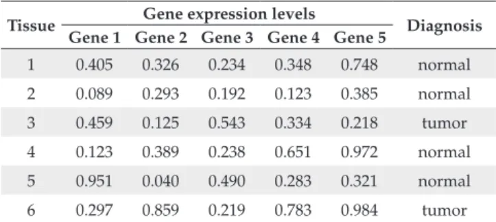
In the experiments reported in this paper, we used data sets obtained from gene expression analysis, particularly tissue classification. Gene expression analysis problems are, in general, represented by complex and high dimensional data sets, which are very susceptible to noise. Table 1 shows the format of the gene expression data sets used in the experi-ments. It shows that each data set can be represented by a table where the first row has the identification of a particular tissue, the expression levels of different genes for this tissue and the label associated to the tissue.
The main features of the gene expression data sets used in the experiments are described in Table 2. This table presents, for each data sets, its total number of instances, number of attributes or data dimensionality and existent classes.
Most of the data sets used in the experiments reported in this paper are related to the problem of cancer tissue classification. The development of efficient data analysis tools to support experts may allow better and earlier
diag-nosis of cancer, leading to more effective patient treatment and increase of survival rates. Several research groups are currently working with gene expression analysis of tumor tissues.
The ExpGen data set4 contains expression levels
measure-ments from 2467 genes obtained from 79 different laboratory experiments for genes functional classification. This applica-tion consists in categorize a gene in a given class that represent its function in the cellular environment. From these experi-ments, the data set is composed by only 207 genes, which could be categorized into five classes during the laboratorial experiments made.
The Golub data set15 has gene expression levels from
patients with acute leukemia. The gene expression data were obtained from 72 microarray images, and measure expres-sion levels of 6817 human genes. The disease was categorized in two different types, Acute Lymphoid Leukemia (ALL) and Acute Myeloid Leukemia (AML). The same pre-processing made in11 was applied to Golub data set to simplify its data.
The Leukemia data set is known in literature as St. Jude Leukemia38. It is composed by six different types of pediatric
acute lymphoid leukemia and another group with examples which could not be categorized as one of the previous six types. The original data set has 12558 genes and so a pre-pro-cessed version found in http://sdmc.lit.org.sg/GEDatasets and described by38 research was used, reducing the number
of genes to 271.
The Lung data set has examples related to lung cancer, where, for each patient, the label can be normal tissue or three different types of lung cancer. The three different types of lung cancer analyzed are adenocarcinomas (ADs), squa-mous cell carcinomas (SQs) and carcinoid (COID). This data set has 197 instances, with 1000 attributes each, and was presented in26.
The last data set analyzed, the Colon data set, is described in Alon et al.2, and includes patients with and without colon
cancer. The data set presents gene expression data obtained from 62 microarrays images, which measure expression levels of 6500 human genes. Pre-processing techniques reduced the number of input attributes to 2000.
For the SVMs training, the SVMTorch II7 software was
employed. The values of different SVMs parameters were the default values of the software used, kept the same for all experiments. For the C4.5, training was carried out by the software provided by Quinlan27 and For the RIPPER
algo-rithm training, the Weka simulator from Waikato university13
was adopted. The parameter values for the three algorithms were the default values suggested in the tools employed, which were kept the same for all experiments. Scripts in perl programming language were also developed to convert data sets to different formats demanded by Wilson’s35 code,
SVMTorch II, Weka simulator and C4.5 algorithm.
To evaluate results obtained in the experiments, the statis-tical test of Friedman14 and Dunn’s multiple comparisons
post-hoc test12 were employed, according to the
method-ology described in10. Friedman’s test was adopted since it is
recommended for the comparison of different ML algorithms Table 1. Format of gene expression data set.
Tissue Gene expression levels Diagnosis Gene 1 Gene 2 Gene 3 Gene 4 Gene 5
1 0.405 0.326 0.234 0.348 0.748 normal
2 0.089 0.293 0.192 0.123 0.385 normal
3 0.459 0.125 0.543 0.334 0.218 tumor
4 0.123 0.389 0.238 0.651 0.972 normal
5 0.951 0.040 0.490 0.283 0.321 normal
6 0.297 0.859 0.219 0.783 0.984 tumor
Table 2. Description of data sets analyzed.
Data set Instances Attributes Classes ExpGen 207 79 B, H, T, R, P
Golub 72 3571 ALL, AML
Leukemia 327 271 BCR, E2A, HYP, MLL, T-ALL, TEL, OTHERS
Lung 197 1000 AD, SQ, COID, NL
applied to multiple data sets, and has the advantage of not assuming that the measurements have to follow a Normal distribution.
The null hypothesis assume that all analyzed algorithms are equivalent if their respective mean ranks are the same. If the null hypothesis is rejected, and therefore the analyzed algorithms are statistically different, a post-hoc test might be applied to detect which of the algorithms differ. Dunn’s statistical post-hoc test was applied, since it is recommended to situations where all algorithms analyzed are compared to a control algorithm, the strategy employed in the experiments performed in this paper.
4. Experimental Results
In the pre-processing, the amount of removed instances was different for each data set analyzed. However, it was between 20 and 30% of the total number, except for the Colon data set, original and simplified versions, which presented reductions between 30 and 40%.
The time spent in the pre-processing phase was meas-ured to show how the application of the noise detection techniques investigated can affect the overall processing time. It is important to mention that pre-processing phase is only applied once for each data set analyzed, generating a pre-processed data set that can be used several times for different ML algorithms. The time consumed was always less than one minute. Another observation is related to data sets complexity: more time was spent in the pre-processing of more complex data sets.
In order to measure the effectiveness of noise detection techniques employed, the performance of the three ML algorithms concerning accuracy, complexity and processing time necessary to build the induced hypothesis were evalu-ated with the original and the pre-processed data. For all experiments, the statistical tests were applied with 95% of confidence level.
For SVMs, in general, the error rates of the classifiers generated after the application of noise detection techniques, for all evaluated k values, were the same as those obtained for the original data sets. The same was true for the Colon data set, but only for some values of k. The pre-processed data sets Leukemia and ExpGen had only some similar results, but none better than those obtained for the original data sets, while Golub data set presented the worst results in all cases. The obtained results can be seen in Table 3, where the best results are highlighted in bold and error rates similar to the best ones for each data set are shown in italics. Standard devi-ation rates are reported in parenthesis.
The analysis of the C4.5 classification error rates, which can be seen in Table 4, shows that the pre-processed data sets Leukemia, Lung and Golub presented similar and better results than those obtained for the original data sets. The ExpGen data set presented only few similar error rates compared to those obtained for the original data set. The pre-processed data set Colon provided only worst results.
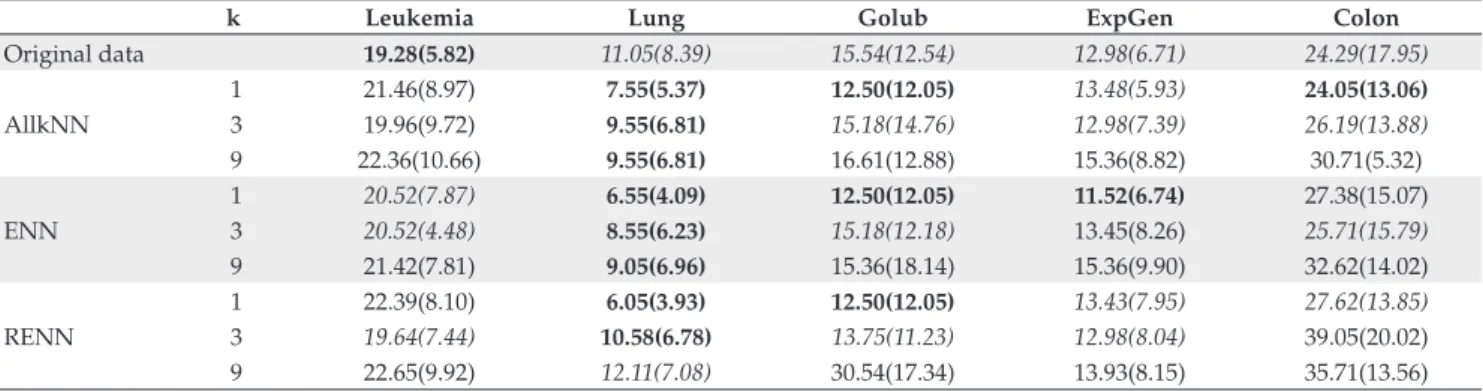
According to Table 5, the RIPPER algorithm presented similar error performance for the original and pre-processed data using the Leukemia, ExpGen and Colon data sets. In the last two data sets, some results were improved by the pre-processing. The remaining pre-processed data sets Lung and Golub presented more improvements in ML accuracy after the pre-processing phase. For these two data sets, error rates were lower after pre-processing, for the majority of the exper-iments carried out.
In the complexity analysis of the SVMs, the number of Support Vectors (SVs), data that determine the decision border induced by SVMs, was considered. A smaller number of SVs indicates less complexity of the induced model.
For the C4.5 algorithm, complexity was determined by the mean decision tree size induced. Reduced decision trees are easier to analyze and so result in comprehensiveness improvements for the model.
The complexity for RIPPER algorithm was observed by the number of rules produced during the training phase. The smaller the number of rules produced, the simpler the complexity of the generated model.
For all three ML algorithms investigated, the complexity was reduced when the pre-processed data sets were used, as presented in Tables 6, 7 and 8, respectively for the SVM, C4.5 and RIPPER algorithms. In these tables, the best results are highlighted in bold and complexities similar to the best ones, for each data set, are shown in italics. Standard devia-tion rates are reported in parenthesis.
According to Tables 6, 7 and 8, most of the complexities were reduced after pre-processing, except for the Golub data set and the RIPPER algorithm, in which not all complexities were reduced.
For the SVMs, the smaller the pre-processed data set produced by noise detection techniques, the lower the number of SVs obtained and, consequently, the complexity of the model. For the C4.5 algorithm, the model complexity has decreased until a lower bound from which further reduction in pre-processed data set would not reduce the complexity.
For the RIPPER algorithm, the final models were also simplified, but with less reduction in the complexity. The complexity obtained using the original data for the Golub data set was maintained for its pre-processed versions.
The time taken by the SVM, C4.5 and RIPPER algorithms to induce hypothesis using the pre-processed data sets was always reduced when compared to those obtained with the original data sets, taking at most 1 second. For SVMs, the processing time was only slightly reduced in comparison to the time obtained for the original data sets.
Table 3. SVMs error rates and standard deviation for the original and pre-processed data sets.
k Leukemia Lung Golub ExpGen Colon
Original data 7.05(4.39) 29.42(3.74) 29.28(10.75) 7.66(6.82) 35.71(13.56) 1 7.95(3.91) 29.42(3.74) 32.14(13.88) 7.69(5.13) 35.71(13.56) AllkNN 3 7.95(3.91) 29.42(3.74) 34.82(13.91) 8.19(3.90) 35.71(13.56) 9 7.94(2.96) 29.42(3.74) 34.82(13.91) 8.69(3.76) 35.71(13.56) 1 7.34(3.65) 29.42(3.74) 32.14(13.88) 8.67(4.34) 35.71(13.56) ENN 3 8.27(3.61) 29.42(3.74) 34.82(13.91) 7.71(3.32) 35.71(13.56) 9 11.00(4.83) 29.42(3.74) 34.82(13.91) 9.64(5.48) 42.38(18.60)
1 7.65(3.93) 29.42(3.74) 32.14(13.88) 8.67(4.34) 35.71(13.56)
RENN 3 11.01(5.08) 29.42(3.74) 34.82(13.91) 7.71(3.32) 44.28(19.35) 9 13.43(6.26) 29.42(3.74) 56.25(20.15) 9.17(4.16) 64.28(13.56)
Table 4. C4.5 error rates and standard deviation for the original and pre-processed data sets.
k Leukemia Lung Golub ExpGen Colon
Original data 17.18(6.98) 9.14(5.22) 16.44(8.12) 8.19(4.60) 20.97(13.45)
1 18.95(5.07) 6.06(5.15) 17.87(8.91) 8.16(7.46) 26.43(21.38) AllkNN 3 17.47(5.51) 7.56(4.21) 13.58(12.69) 8.65(4.91) 24.52(11.48)
9 18.70(5.58) 7.56(4.21) 11.97(14.24) 12.52(5.07) 30.70(5.29) 1 17.43(4.75) 5.56(4.97) 16.44(10.54) 9.18(6.10) 21.43(19.40) ENN 3 16.83(7.05) 8.08(4.83) 13.58(12.69) 12.03(7.47) 30.00(17.52) 9 17.43(6.19) 8.08(6.32) 11.08(12.66) 12.49(7.07) 32.86(19.30) 1 17.74(4.87) 6.06(4.58) 16.44(10.54) 9.66(6.32) 28.58(23.47) RENN 3 16.83(6.72) 7.58(4.87) 13.58(12.69) 12.50(7.10) 40.72(14.91) 9 16.81(4.98) 9.13(4.59) 29.48(18.04) 12.49(7.07) 35.72(13.55)
Table 5. Error rates and standard deviation of RIPPER algorithm applied to original and pre-processed data sets.
k Leukemia Lung Golub ExpGen Colon
Original data 19.28(5.82) 11.05(8.39) 15.54(12.54) 12.98(6.71) 24.29(17.95) 1 21.46(8.97) 7.55(5.37) 12.50(12.05) 13.48(5.93) 24.05(13.06) AllkNN 3 19.96(9.72) 9.55(6.81) 15.18(14.76) 12.98(7.39) 26.19(13.88) 9 22.36(10.66) 9.55(6.81) 16.61(12.88) 15.36(8.82) 30.71(5.32) 1 20.52(7.87) 6.55(4.09) 12.50(12.05) 11.52(6.74) 27.38(15.07) ENN 3 20.52(4.48) 8.55(6.23) 15.18(12.18) 13.45(8.26) 25.71(15.79)
9 21.42(7.81) 9.05(6.96) 15.36(18.14) 15.36(9.90) 32.62(14.02) 1 22.39(8.10) 6.05(3.93) 12.50(12.05) 13.43(7.95) 27.62(13.85) RENN 3 19.64(7.44) 10.58(6.78) 13.75(11.23) 12.98(8.04) 39.05(20.02)
9 22.65(9.92) 12.11(7.08) 30.54(17.34) 13.93(8.15) 35.71(13.56)
Table 6. Mean number of SVs produced by SVMs applied to original and pre-processed data sets.
k Leukemia Lung Golub ExpGen Colon
Original data 49.6(0.94) 177.3(0.48) 64.8(0.42) 35.7(1.09) 55.8(0.42) 1 40.0(0.90) 151.1(2.08) 54.6(0.70) 26.9(1.78) 38.8(2.97) AllkNN 3 38.1(1.56) 150.7(1.94) 51.9(1.91) 24.7(2.25) 34.3(2.67) 9 37.4(1.37) 149.6(2.17) 49.0(2.16) 22.5(1.85) 29.9(2.51) 1 40.3(0.68) 152.7(1.94) 54.8(0.92) 27.3(1.90) 39.4(3.10)
ENN 3 38.1(1.21) 153.5(1.08) 53.0(1.56) 25.3(2.88) 35.4(1.43)
9 36.5(1.35) 152.5(1.35) 49.1(2.51) 22.9(1.07) 27.5(14.56) 1 40.0(0.84) 152.3(2.62) 54.8(0.92) 26.3(2.18) 38.3(4.24) RENN 3 37.5(2.61) 150.6(2.87) 52.7(1.89) 24.1(2.30) 19.0(16.43)
Table 7. Mean decision tree size produced by C4.5 algorithm applied to original and pre-processed data sets.
k Leukemia Lung Golub ExpGen Colon
Original data 34.20(2.15) 9.40(0.84) 4.40(0.96) 14.00(1.41) 6.80(0.63)
1 24.60(2.27) 7.00(0.00) 4.00(1.05) 9.00(0.94) 4.40(0.96) AllkNN 3 21.40(1.84) 7.00(0.00) 3.40(0.84) 7.80(1.03) 3.40(0.84) 9 18.80(1.47) 7.00(0.00) 3.40(0.84) 7.00(0.00) 2.80(0.63) 1 23.80(1.68) 7.20(0.63) 4.00(1.05) 8.60(0.84) 4.40(0.96)
ENN 3 21.60(1.35) 7.00(0.00) 3.40(0.84) 8.60(0.84) 3.60(0.96)
9 19.00(1.34) 7.00(0.00) 3.40(0.84) 8.20(1.40) 2.20(1.03) 1 22.40(2.12) 7.00(0.00) 4.00(1.05) 8.60(0.84) 4.40(0.96) RENN 3 19.80(1.40) 7.00(0.00) 3.40(0.84) 8.40(0.96) 2.20(1.03) 9 17.00(0.94) 6.80(0.63) 2.00(1.70) 8.00(1.41) 1.00(0.00)
Table 8. Mean number of rules produced by RIPPER algorithm applied to original and pre-processed data sets.
k Leukemia Lung Golub ExpGen Colon
Original data 10.80(1.40) 5.00(0.67) 2.10(0.31) 5.70(0.67) 3.00(0.67) 1 9.30(1.06) 4.10(0.31) 2.20(0.42) 4.80(0.42) 2.40(0.51) AllkNN 3 8.70(1.06) 4.00(0.00) 2.30(0.48) 4.70(0.67) 2.40(0.51) 9 8.00(0.94) 4.00(0.00) 2.10(0.31) 4.10(0.57) 1.60(0.51) 1 9.60(1.07) 4.10(0.31) 2.20(0.42) 5.10(0.74) 2.30(0.48)
ENN 3 9.10(1.45) 4.10(0.31) 2.20(0.42) 4.70(0.67) 2.10(0.31)
9 7.80(0.79) 4.20(0.42) 2.20(0.00) 4.40(0.84) 1.20(0.42) 1 9.60(0.96) 4.00(0.00) 2.20(0.00) 5.20(0.79) 2.40(0.51) RENN 3 8.80(0.92) 4.10(0.31) 2.10(0.31) 4.70(0.67) 1.30(0.48) 9 7.90(0.56) 4.10(0.57) 1.30(0.48) 4.20(0.63) 1.00(0.00)
in these algorithms may not result in significant differences in the ML algorithms performance.
Most of the experiments presented satisfactory results, with lower error rates and better performance if compared to those obtained in the analysis of the original data sets, which demonstrates that noise detection techniques improved the performance of the ML algorithms evaluated. The C4.5 and RIPPER algorithms benefited from the application of noise detection techniques for most of the data sets investigated and reduced the complexity of the induced models. For the SVMs, the new results were slightly better, with lower complexity.
Furthermore, the gain in comprehensiveness and the reduction in time spent during training process is another advantage, since the complexities of all data sets were reduced after pre-processing (the noise detection and removal phase).
Therefore, the application of noise detection techniques in a pre-processing phase presents the advantage of reducing the complexity of classifiers induced by ML algorithms, as well as reducing the time spent in classifiers training, producing, in most experiments, better or similar classifica-tion error results than those obtained for the original data sets. This indicates that the distance-based noise detection techniques kept the most expressive patterns of the data sets and allowed ML algorithms to induce simpler classifiers, as shown in the reduced complexity and lower classification error rates obtained.
5. Conclusions
This paper investigated the application of distance-based noise detection techniques in different gene expression classi-fication problems. We did not found in the literature a single approach or algorithm able to detect noise without classifica-tion accuracy reducclassifica-tion that was tested in several data sets. We also were not able to find noise detection experiments using gene expression data sets able to detect tissues that are probably noise. The closest works we found in gene expres-sion analysis were the works from18, 24. However, these works
detect and eliminate only genes, not tissues. The data sets employed here are related to both gene classification and tissue classification.
In the experiments performed here, three ML algorithms were trained over the original and pre-processed data sets. They were employed to evaluate the power of these tech-niques in maintaining the most informative patterns. The results observed indicate that the noise detection techniques employed were effective in the noise detection process. These experiments shown the the incorporation of noise detection and elimination resulted in simplifications of the ML classifiers and in reduction in their classification error rates, specially for the C4.5 and RIPPER algorithms. Another advantage for these two algorithms was an increase in comprehensiveness.
detec-tion techniques aiming to further improve the gains obtained by the identification and removal of noisy data. Preliminary results, presented in Libralon23, suggest that ensembles of
distance-based techniques can be a good alternative for noise detection in gene expression data sets.
Acknowledgements
The authors would like to thank the São Paulo State Research Foundation (FAPESP) and CNPq for the financial support provided.
References
1. Aggarwal CC, Hinneburg A, Keim DA. On the surprising behavior of distance metrics in high dimensional space. In: Proceedings of the 8th Int. Conf. on Database Theory, LNCS - vol. 1973; 2001; London. Springer-Verlag; 2001. p. 420-434.
2. Alon U, Barkai N, Notterman DA, Gish K, Ybarra S, Mack D, Levine AJ. Broad Patterns of Gene Expression Revealed by Clustering Analysis of Tumor and Normal Colon Tissues Probed by Oligonucleotide Arrays. In: Proceedings of National Academy of Sciences of the United States of America; 1999. USA: The National Academy of Sciences; 1999. p. 6745-6750.
3. Barnett V, Lewis T. Outliers in statistical data. 3 ed. New York: Wiley Series in Probability & Statistics, John Wiley and Sons; 1994.
4. Brown M, Grundy W, Lin D, Christianini N, Sugnet CM Jr., Haussler D. Support vector machine classification of microarray gene expression data. Santa Cruz, CA 95065: University of California; 1999. Technical Report UCSC-CRL-99-09.
5. Chien-Yu C. Detecting homogeneity in protein sequence clusters for automatic functional annotation and noise detection. In: Proceedings of the 5th Emerging Information Technology Conference; 2005; Taipei.
6. Cohen WW. Fast effective rule induction. In: Proceedings of the 12th International Conference on Machine Learning; 1995. Tahoe City, CA: Morgan Kaufmann; 1995. p. 115-123.
7. Collobert R, Bengio S. SVMTorch: support vector machines for large-scale regression problems. The Journal of Machine Learning Research 2001; 1:143-160.
8. Corney DPA. Intelligent analysis of small data sets for food design. London: Computer Science Department, London University College; 2002.
9. Cristianini N, Shawe-Taylor J. An introduction to support vector machines and other kernel-based learning methods. Cambridge: Cambridge University Press; 2000.
10. Demsar J. Statistical comparisons of classifiers over multiple datasets. Journal of Machine Learning Research 2006; 7:1-30.
11. Dudoit S, Fridlyand J, Speed TP. Comparison of discrimination methods for the classication of tumors using gene expression data. UC Berkeley: Department of Statistics; 2000. Technical Report 576.
12. Dunn OJ. Multiple comparisons among means. Journal of American Statistical Association 1961; 56(293):52-64.
13. Frank E, Witten IH. Data mining: practical machine learning tools and techniques. San Francisco: Morgan Kaufmann; 2005.
14. Friedman M. The use of ranks to avoid the assumption of normality implicit in the analysis of variance. Journal of American Statistical Association 1937; 32(200):675-701.
15. Golub TR, Tamayo P, Slonim D, Mesirow J, Zhu Q, Kitareewan S, Dmitrovsky E, Lander ES. Interpreting patterns of gene expression with self-organizing maps: Methods and application to hematopoietic differentiation. In: Proceedings of National Academy of Sciences; 1999. USA: The National Academy of Sciences; 1999; 96(6):2907-2912.
16. He Z, Xu X, Deng S. Discovering cluster-based local outliers. Pattern Recognition Letters 2003; 24(9-10):1641-1650.
17. Hodge V, Austin J. A survey of outlier detection methodologies. Artificial Intelligence Review 2004; 22(2):85-126.
18. Hu J. Cancer outlier detection based on likelihood ratio test. Bioinformatics 2008; 24(19):2193-2199.
19. Khoshgoftaar TM, Rebours P. Generating multiple noise elimination filters with the ensemble-partitioning filter. In: Proceedings of the IEEE International Conference on Information Reuse and Integration; 2004. p. 369-375.
20. Knorr EM, Ng RT, Tucakov V. Distance-based outliers: algorithms and applications. The VLDB Journal 2000; 8(3-4):237-253.
21. Lavrac N, Gamberger D. Saturation filtering for noise and outlier detection. In: Proceedings of the Workshop in Active Learning, Database Sampling, Experimental Design: Views on Instance Selection, 12th European Conference on Machine Learning; 2001. p. 1-4.
22. Lorena AC, Carvalho ACPLF. Evaluation of noise reduction techniques in the splice junction recognition problem. Genetics and Molecular Biology 2004; 27(4):665-672.
23. Libralon GL, Lorena AC, Carvalho ACPLF. Ensembles of pre-processing techniques for noise detection in gene expression data. In: Proceedings of 15th International Conference on Neural Information Processing of the Asia-Pacific Neural Network Assembly; ICONIP2008; Auckland, New Zealand. 2008. p. 1-10.
24. Liu W. Outlier detection for microarray data. In: Proceedings of the 2nd International Conference on Bioinformatics and Biomedical Engineering– ICBBE; 2008; Shanghai. p. 585-586.
25. Mitchell T. Machine learning. USA: McGraw Hill; 1997.
26. Monti S, Tamayo P, Mesirov J, Golub T. Consensus clustering: a resampling-based method for class discovery and visualization of gene expression microarray data. Machine Learning 2003; 52(1-2):91-118.
27. Quinlan JR. C4.5: programs for machine learning. San Francisco, CA: Morgan Kaufmann; 1993.
28. Schlkopf B. SVMs: a practical consequence of learning theory. IEEE Intelligent Systems 1998; 13(4):36-40.
29. Stanfill C, Waltz D. Toward memory-based reasoning. Communications of the ACM 1986; 29(12):1213-1228.
Conference on Knowledge Discovery and Data Mining; 2002; Taipei. p. 535-548.
31. Tomek I. Two modifications of CNN. IEEE Transactions on Systems, Man and Cybernetics 1976; 7(11):769-772.
32. Van Hulse JD, Khoshgoftaar TM, Huang H. The pairwise attribute noise detection algorithm. Knowledge and Information Systems 2007; 11(2):171-190.
33. Vapnik VN. The nature of statistical learning theory. 2 ed. Berlim: Springer-Verlag; 1995.
34. Verbaeten S, Assche AV. Ensemble methods for noise elimination in classification problems. In: Proceedings of the 4th International Workshop on Multiple Classifier Systems; 2003. Berlim: Springer; 2003. p. 317-325.
35. Wilson DR, Martinez TR. Reduction techniques for instance-based learning algorithms. Machine Learning 2000; 38(3):257-286.
36. Wilson DR, Martinez TR. Improved heterogeneous distance functions. Journal of Artificial Intelligence Research 1997; 6(1):1-34.
37. Wilson DL. Asymptotic properties of nearest neighbor rules using edited data. IEEE Transactions on Systems, Man and Cybernetics 1972; 2(3):408-421.