Cost Optimization for Series-Parallel Petroleum Transportation Pape-Lines under Reliability Constraints

Cost Optimization for Series-Parallel Petroleum Transportation

Pape-Lines under Reliability Constraints

M. Amara, R. Meziane, A. Zeblah

Abstract

This paper uses an ant colony meta-heuristic optimization method to solve the cost-optimization problem in petrolum industry. This problem is known as total investment-cost minimization of series-parallel transportation pape lines. Redundant Electro-Pumpe coupled to the papes lines are included to achieve a desired level of availability. System availability is represented by a multi-state availability function. The Electro-pumpe (pape-lines) are characterized by their capacity, availability and cost. These electro-pumpes are chosen among a list of products available on the market. The proposed meta-heuristic seeks to find the best minimal cost of petrol transportation system configuration with desired availability. To estimate the series-parallel pape lines availability, a fast method based on universal moment generating function (UMGF) is suggested. The ant colony approach is used as an optimization technique. An example of petrol transportation system is presented.

Index Terms

—Ant colony; Electro-pumpe; Redundancy optimization; Multi-state systems; Universal generating function (UMGF), petrol transportation

I.

I

NTRODUCTION

One of the most important problems in petrole industry is the redundancy optimization problem. This latter is well known combinatorial optimization problem where the design goal is achieved by discrete choices made from papes available on the market. The natural objective function is to find the minimal cost configuration of a series-parallel petrole transportation pape lines system under availability constraints. The system is considered to have a range of performance levels. In this case the system is called a multi-state system (MSS). Let consider a multi-state pape lines system containing n subsystems Ci (i = 1, 2, …, n) in series

arrangement. For each subsystem Ci there are various

versions, which are proposed by the suppliers on the market. Electro-pumpe (pape lines) are characterized by their cost, capacity and availability according to their version. For example, these electro-pumpess can represent Electro-pumpes coupled to the pape lines in petrole station system to accomplish a task on fluide in our case they represent the chain of electro-pumpes and papes crring systems (Electo-pumpe station, transportation pape lines, ect..). Each subsystem Ci

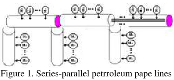
contains a number of electro-pumpe coupled to the pape lines connected in parallel, then a second station put in series ect... Different versions of electro-pumpes may be chosen for any given subsystem. Each subsystem can contain electro-pumpes of different versions as sketched in figure 1.

Figure 1. Series-parallel petrroleum pape lines transportation

1.1-Previous Work

The vast majority of classical reliability or availability analysis and optimization assume that electro-pumpes and system are in either of two states (i.e., complete working state and total failure state). However, in many real life situations we are actually able to distinguish among various levels of performance (capacity) for both system and electro-pumpess. For such situation, the existing dichotomous model is a gross oversimplification and so models assuming multi-state (degradable) systems and electro-pumpess are preferable since they are closer to reliability. Recently much works treat the more sophisticated and more realistic models in which systems and electro-pumpess may assume many states ranging from perfect functioning to complete failure. In this case, it is important to develop MSS reliability theory. In this paper, an MSS reliability theory will be used, where the binary state system theory is extending to the multi-state case. As is addresses in recent review of the literature for example in [1] or [2]. Generally, the methods of MSS reliability assessment are based on four different approaches:

(i)-The structure function approach, (ii)-The stochastic process, (iii)-The Monte-Carlo simulation technique, (iv)-The universal moment generating function (UMGF) approach. In reference [1], a comparison between these four approaches highlights that the UMGF approach is fast enough to be used in the optimization problems where the search space is sizeable.

The problem of total investment-cost minimization, subject to reliability constraints, is well known as the redundancy optimization problem (ROP). The ROP is studied in many different forms as summarized in [3], and more recently in [4]. The ROP for the multi-state reliability was introduced in [5]. In [6] and [7], genetic algorithms were used to find the optimal or nearly optimal transformation system structure. This work uses an ant colony optimization approach to solve the ROP for multi-state petroleum transpot system. The idea of employing a colony of cooperating agents to solve combinatorial optimization problems was recently proposed in [8]. The ant colony approach has been successfully applied to the classical travelling salesman problem in [9], and to the quadratic assignment problem in [10]. Ant colony shows very good results in each applied area. It has been recently adapted for the reliability design of binary state systems in [11]. The ant colony has also been adapted with success to other combinatorial optimization problems such as the vehicle routing problem in [12]. The ant colony method has not yet been used for the redundancy optimization of multi-state systems.

1.2- Approach and Aoutlines

The problem formulated in this paper lead to a complicated combinatorial optimization problem. The total number of different solution to be examined is very large, even for rather small problems. An exhaustive examination of all possible solutions is not feasible given reasonable time limitations. Because of this, the ant colony optimization (or simply ACO) approach is adapted to find optimal or nearly optimal solutions to be obtained in a short time. The newer developed meta-heuristic method has the advantage to solve the ROP for MSS without the limitation on the diversity of versions of electro-pumpess in parallel. During the optimization process, artificial ants will have to evaluate the availability of a given selected structure of the series-parallel petroleum transport system. To do this, a fast procedure of availability estimation is developed. This procedure is based on a modern mathematical technique: the z-transform or UMGF which was introduced in [13]. It was proven to be very effective for high dimension combinatorial problems: see e.g., in [2]. The universal moment generating function is an extension of the ordinary

moment generating function (UGF) in [14]. The method developed in this paper allows the availability function of reparable series-parallel MSS to be obtained using a straightforward numerical procedure. The rest of this paper is outlined as follows. We start in section 2 with the formulation of the optimization problem of petrole transportation. In section 3, we develop the reliability estimation of a series-parallel multi-state petroleum system method. In section 4, we describe the ant colony optimization approach to solve the redundancy optimization problem of petrole transportation industry. In section 5, illustrative examples and numerical results are presented in which the optimal choice of pape-lines in a system is found. Conclusions are drawn in section 6.

II.

F

ORMULATION

O

F

T

HE

O

PTIMIZATION

P

ROBLEM

O

F

P

ETROLEUM

T

RANSPORTATION

S

YSTEM Let consider a series-parallel petrole transportation system containing n subsystems Ci (i =

1, 2, …, n) in series arrangement as represented in figure 1. Every subsystem Ci contains a number of

different Electro-pumpe (pipe-lines) connected in parallel. For each subsystem i, there are a number of Electro-pumpe versions available in the market. For any given system Electro-pumpe, different versions and number of Electro-pumpes may be chosen. For each subsystem i, Electro-pumpes are characterized according to their version v by their cost (Civ),

availability (Aiv) and capacity or (Debit) (iv). The

structure of subsystem

i

can be defined by the numbers of parallel Electro-pumpes (of each version)

iv

k

for 1vV_i, where

V

_i is a number of versions available for Electro-pumpes of type i. Figure 1 illustrates these notations for a given subsystem i. The entire system structure is defined by the vectors ki =

 

kiv_i (1in,1vVi). For a given set of

vectors k1, k2, …, kn the total cost of the system can

be calculated as:

 

   n

1 i

V

1 v

iv iv

i C k

C (1)

2.1-Reliability of reparable multi-states petroleum system

but not to complete failure. An important MSS measure is related to the ability of the system to satisfy a given demand.

For instance in electric power systems, reliability is considered as a measure of the ability of the system to meet the load demand (D), i.e., to provide an adequate supply of electrical energy (฀). This definition of the reliability index is widely used in power systems: see e.g., in [14,15,16] and in [6-7]. The Loss of Load Probability index (LOLP) is usually used to estimate the reliability index in [17]. This index is the overall probability that the load demand will not be met. Thus, we can write R = Probab( D) or R = 1-LOLP with LOLP = Probab( D). This reliability index depends on consumer demand D. For reparable MSS, a multi-state steady-state availability E is used as Probab(  D) after enough time has passed for this probability to become constant in [16]. In the steady-state the distribution of states probabilities is given by equation (2), while the multi-state stationary availability is formulated by equation (3):

Pj = lim[Probab( j)]

t



(

t

)





(2)



 

 D

j

j

P

E (3)

If the operation period T is divided into

M

intervals (with duration's T1, T2, …, TM) and

each interval has a required demand level (D1, D2, …,

DM , respectively), then the generalized MSS

availability index A is:

j M

1 j

j M

1 j

j

T ) D ( obab Pr T 1

A









 

 (4)

We denote by D and T the vectors

 

Dj and

 

T j

(1jM), respectively. As the availability A is a function of k1, k2, …, kn, D and T, it will be written

A(k1, k2, …, kn, D, T). In the case of a power system,

the vectors D and T define the cumulative load curve (consumer demand). In reality the load curves varies randomly; an approximation is used from random curve to discrete curve see in [18]. In general, this curve is known for every power system.

2.2- Optimal design optimisation

The multi-state petroleum transport system redundancy optimization problem can be formulated as follows: find the minimal cost system configuration k1, k2, …, kn, such that the corresponding availability

exceeds or equal the specified availability A0. That is,

Minimize

 

   n

1 i

V

1 v iv iv

i C k

C (5) Subject to

A(k1, k2, …, kn, D, T) A0 (6)

The input of this problem is the specified availability and the outputs are the minimal investment-cost and the corresponding transport petroleum configuration. To solve this combinatorial optimization problem, it is important to have an effective and fast procedure to evaluate the availability index for a series-parallel plastic transport petroleum system. Thus, a method is developed in the next section to estimate the value of A(k1, k2, …, kn,

D, T).

III.

M

ULTI

-S

TATES

A

VAILABILITY

E

STIMATION

The procedure used in this paper is based on the universal z-transform, which is a modern mathematical technique introduced in [13]. This method, convenient for numerical implementation, is proved to be very effective for high dimension combinatorial problems. In the literature, the universal z-transform is also called universal moment generating function (UMGF) or simply u-function or u-transform. In this paper, we mainly use the acronym UMGF. The UMGF extends the widely known ordinary moment generating function in [14].

The UMGF of a discrete random variable  is defined as a polynomial:

j z P ) z ( u

J

1 j j







 (7)

where the variable ฀ has J possible values and P is j

the probability that ฀ is equal to ฀j.

The probabilistic characteristics of the random variable ฀ can be found using the function u(z). In particular, if the discrete random variable ฀ is the MSS stationary output performance, the availability E is given by the probability Probab(฀  D) which can be defined as follows:



_u(z)z D



) D

Probab(   ₍₈₎

where  is a distributive operator defined by expressions (9) and (10):

   

 

  

 

D if , 0

D if , P ) Pz









      _{ }          J 1 j D j J 1 j D j j

j _Pz

z P

(10)

It can be easily shown that equations (7)–(10) meet condition Probab(฀  D)=



  D

j

j

P . By using the

operator



, the coefficients of polynomial u(z) are summed for every term with ฀j  D, and the

probability that ฀ is not less than some arbitrary value D is systematically obtained. Consider single pumpess with total failures and each electro-pumpes i has nominal performance ฀i and availability

Ai. Then, Probab(฀ = ฀i) = Ai and Probab(฀ = ) = i

A

1 . The UMGF of such an electro-pumpes has only two terms can be defined as:

i z A z ) A 1 ( ) z ( u i 0 i i   

 = _{(1 A) Az} i

i i





 (11)

To evaluate the MSS availability of a series-parallel system, two basic composition operators are introduced. These operators determine the polynomial u(z) for a group of electro-pumpess.

- parallel Electro-Pumpes

Let consider a subsystem m containing Jm

electro-pumpess connected in parallel. As the performance measure is related to the system productivity, the total performance of the parallel subsystem is the sum of performances of all its electro-pumpess. In power systems engineering, the term capacity is usually used to indicate the quantitative performance measure of an electro-pumpes in [6]. It may have different physical nature. Examples of electro-pumpess capacities are: generating capacity for a generator, pipeline capacity for a water circulator, carrying capacity for an electric transmission line, etc. The capacity of an electro-pumpes can be measured as a percentage of nominal total system capacity. In a electrical network, electro-pumpess are generators, transformers and electrical lines. Therefore, the total performance of the parallel electro-pumpes is the sum of performances in [19]. The u-function of MSS subsystem m containing Jm

parallel electro-pumpess can be calculated by using the  operator:

)) z ( u ..., ), z ( u ), z ( u ( ) z (

up  1 2 n ,where



   n 1 i i n 2

1, g , ..., g ) g

g

( .

Therefore for a pair of electro-pumpess connected in parallel: )) z ( u ), z ( u

( 1 2

 = ( Pz , Q z )

m 1 j b j n 1 i a i j i





   =



   n 1 i m 1 j b a j i j i z Q P .

Parameters ai and bj are physically interpreted as the

respective performances of the two electro-pumpess. n and m are numbers of possible performance levels for these electro-pumpess. Pi and Qj are steady-state

probabilities of possible performance levels for electro-pumpess.

One can see that the  operator is simply a product of the individual u-functions. Thus, the subsystem UMGF is:





Jm

1 j

j p(z) u (z)

u

Given the individual UMGF of electro-pumpess defined in equation (11), we have:



     m i J 1 j j j

p(z) (1 A Az )

u .

- Series Electro-Pumpes

When the electro-pumpess are connected in series, the electro-pumpes with the least performance becomes the bottleneck of the system. This electro-pumpes therefore defines the total system productivity. To calculate the u-function for system containing n subsystems connected in series, the operator

 should be used:

)) z ( u ..., ), z ( u ), z ( u ( ) z (

us  1 2 m , where



1 2 m



m 2

1, g , ...,g ) ming, g ,..., g

g

( 

 so that





 





                n 1 i m 1 j b , a m in j i m 1 j b j n 1 i a i 2 1 j i j i z Q P z Q , z P )) z ( u ), z ( u (

Applying composition operators  and  consecutively, one can obtain the UMGF of the entire series-parallel system. To do this we must first determine the individual UMGF of each electro-pumpes.

- Electro-Pumpes with total failures

Let consider the usual case where only total failures are considered (K = 2) and each electro-pumpes of type i and version vi has nominal

performance ฀iv and availability Aiv. In this case, we

have:

Probab(฀ = ฀iv) = Aiv and Probab(฀ = ) = 1Aiv.

terms and can be defined as in equation (11) by

iv

z A z ) A 1 ( ) z (

u*i   _iv 0 _iv  = 1A_ivA_ivziv.

Using the  operator, we can obtain the UMGF of the i-th system electro-pumpes containing ki

parallel electro-pumpess as u_i(z)

 

u*i(z)ki =



_iv



ki

iv ivz (1 A )

A    .

The UMGF of the entire system containing n electro-pumpess connected in series is:















  

 

    

 

 

 

  



  

n nv

2 v

2

1 v

1

k nv nv

k v 2 v

2

k v 1 v

1

s

) A 1 ( z A ..., ,

) A 1 ( z A

, ) A 1 ( z A

) z (

u (12)

To evaluate the probability Probab(฀  D) for the entire system, the operator



is applied to equation (12):

Probab(฀  D) =



us(z)z D





 (13)

The above procedure was implemented and tested on a PC computer and shown to be effective and fast. The UMGF method, convenient for numerical implementation, is efficient for the high dimension combinatorial problem formulated in this work. In our optimization technique to solve this problem, artificial ants will evaluate the availability of given selected structures of the series-parallel transport petroleum system. To do this, the fast implemented procedure of availability estimation will be used by the optimization program. The next section presents the ant colony meta-heuristic optimization method to solve the redundancy optimization problem for multi-state plastic transport petroleum systems.

IV.

T

HE

A

NT

C

OLONY

A

PPROACH The problem formulated in this paper is a complicated combinatorial optimization problem. The total number of different solutions to be examined is very large, even for rather small problems. An exhaustive examination of the enormous number of possible solutions is not feasible given reasonable time limitations. Thus, because of the search space size of the ROP for MSS, a new meta-heuristic is developed in this section. This meta-heuristic consists in an adaptation of the ant colony optimization method.

The ACO principal

Recently, in [8] introduced a new approach to optimization problems derived from the study of

any colonies, called ―Ant System‖. Their system inspired by the work of real ant colonies that exhibit the highly structured behavior. Ants lay down in some quantity an aromatic substance, known as pheromone, in their way to food. An ant chooses a specific path in correlation with the intensity of the pheromone. The pheromone trail evaporates over time if no more pheromone in laid down by others ants, therefore the best paths has more intensive pheromone and higher probability to be chosen. This simple behavior explains why ants are able to adjust to changes in the environment, such as new obstacles interrupting the currently shortest path.

Artificial ants used in ant system are agents with very simple basic capabilities mimic the behavior of real ants to some extent. This approach provides algorithms called ant algorithms. The Ant System approach associates pheromone trails to features of the solutions of a combinatorial problem, which can be seen as a kind of adaptive memory of the previous solutions. Solutions are iteratively constructed in a randomized heuristic fashion biased by the pheromone trails, left by the previous ants. The pheromone trails, ij , are updated after the

construction of a solution, enforcing that the best features will have a more intensive pheromone. An Ant algorithm presents the following characteristics. It is a natural algorithm since it is based on the behavior of ants in establishing paths from their colony to feeding sources and back. It is parallel and distributed since it concerns a population of agents moving simultaneously, independently and without supervisor. It is cooperative since each agent chooses a path on the basis of the information, pheromone trails, laid by the other agents with have previously selected the same path. It is versatile that can be applied to similar versions the same problem. It is robust that it can be applied with minimal changes to other combinatorial optimization problems. The solution of the travelling salesman problem (TSP) was one of the first applications of ACO.

ACO-based Solution Approach

In our reliability optimization problem, we have to select the best combination of parts to minimize the total cost given a reliability constraint. The parts can be chosen in any combination from the available electro-pumpess. Electro-pumpess are characterized by their reliability, capacity and cost. This problem can be represented by a graph (figure 2) in which the set of nodes comprises the set of subsystems and the set of available electro-pumpess (i.e. max (Mj), j = 1..n) with a set of connections

partially connect the graph (i.e. each subsystem is connected only to its available electro-pumpess). An additional node (blank node) is connected to each subsystem

Figure 2. Series-Parallel Petrroleum Pape Lines Transportation Represented In Graph

In figure 2, a series-parallel petroleum transport system is illustrated. At each step of the construction process, an ant uses problem-specific heuristic information, denoted by ij to choose the

optimal number of electro-pumpess in each subsystem. Imaginary heuristic information is associated to each blank node. These new factors allow us to limit the search surfaces (i.e. tuning factors). An ant positioned on subsystem i chooses a electro-pumpes j by applying the rule given by:









_

_

_



  

o o im

im AC m

q

q

if

J

q

q

if

)

]

[

]

([

max

arg

j

i



(14)

and J is chosen according to the probability:

   

   





























 

 

otherwise

0

AC

j

if

p

i

AC m

im im

ij ij

ij

i (15)

 : The relative importance of the trail.

 : The relative importance of the heuristic information ij.

ACi: The set of available electro-pumpess choices for

subsystem i.

q: Random number uniformly generated between 0 and 1.

The heuristic information used is : ij =

1/(1+cij) where cij represents the associated cost of

electro-pumpes j for subsystem i. A ―tuning‖ factor ti= ij = 1/(1+ci(Mi+1)) is associated to blank

electro-pumpes (Mi+1) of subsystem i. The parameter qo

determines the relative importance of exploitation versus exploration: every time an ant in subsystem i have to choose a electro-pumpes j, it samples a random number 0q1. If qqo then the best edge,

according to (14), is chosen (exploitation), otherwise an edge is chosen according to (15) (biased exploration).

The pheromone update consists of two phases: local and global updating. While building a solution of the problem, ants choose electro-pumpess and change the pheromone level on subsystem-electro-pumpes edges. This local trail update is introduced to avoid premature convergence and effects a temporary reduction in the quantity of pheromone for a given subsystem-electro-pumpes edge so as to discourage the next ant from choosing the same electro-pumpes during the same cycle. The local updating is given by:

o old ij new

ij (1) 

 (16)

where  is a coefficient such that (1-) represents the evaporation of trail and ois an initial value of trail

intensity. It is initialized to the value (n.TCnn)-1 with n

is the size of the problem (i.e. number of subsystem and total number of available electro-pumpes) and TCnn is the result of a solution obtained through some

simple heuristic.

After all ants have constructed a complete system, the pheromone trail is then updated at the end of a cycle (i.e. global updating), but only for the best solution found. This choice, together with the use of the pseudo-random-proportional rule given by (14) and (15), is intended to make the search more directed: ants search in a neighborhood of the best solution found up to the current iteration of the algorithm. The pheromone level is updated by applying the following global updating rule:

ij old ij new

ij (1) 

 (17)

   

 _

  

otherwise 0

tour best ) j , i ( if TC

1

best

ij (18)

-The Algorithm

subsystem according to the Pseudo-random-proportional transition rule given by (14) and (15). When an ant selects a electro-pumpes, a local update is made to the trail for that subsystem-electro-pumpe edge according to equation (16). In this equation,  is a parameter that determines the rate of reduction of the pheromone level. The pheromone reduction is small but sufficient to lower the attractiveness of precedent subsystem-electro-pumpe edge. At the end

of a cycle, for each ant k, the value of the system‘s

reliability Ak and the total cost TCkare computed. The

best feasible solution found by ants (i.e. total cost and assignments) is saved. The pheromone trail is then updated for the best solution obtained according to (17) and (18). This process is iterated until the tour counter reaches the maximum number of cycles NCmax or all ants make the same tour (stagnation

behavior).

V.

I

LLUSTRATIVE

E

XAMPLE 1) Description of The System to be Optimized

In order to illustrate the proposed ant colony algorithm, a petroleum transportation pape-lines system is considered.

The petroleum feeding system station (Gaz or quandonsa liquid) supplies the boat transport. It consists of five basic subsystems (type of parallel electro pumpe coupled to diferrent section pape-lines).

1- Reservoir 1is composed by a set of parallel electro-pumpes, loads the liquid from reservoir to the first station distrubutor where it is evacuated. 2- The first station is composed by electro-pumpes

to carry the liquid and supply the second stations. 3- The second station accumulate the gaz or liquid which is distrubuate to other pape-lines with different sections with high debit by a specific electro-pumpes.

4- The third station received and select between different density of Gaz or liquid (rafiner) and supply the four station.

5- In the end the four station condense the Gaz and transform it to liquid with a set of refrigirator electro-pumpe and loded it to the boat transport. Each electro-pumpe of the system is considered as unit with one mode failures.

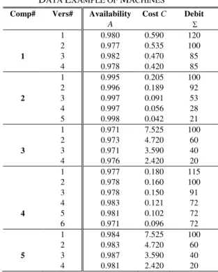
Table 1 shows the numerical data for each electro-pumpe. Each electro-pumpe of the subsystem is considered as a unit with total failures. Table 2 contains the data of cumulative demand.

The numbers of machines Chmax in parallel

are set to (4,5,4,6,4). The number of ants used to find the best solution is 30. The simulation results depend greatly on the values of the coefficients  and . Different ti values (tuning factors associated to blank

electro-pumpess) were tested and shown to influence

greatly the algorithm. The best found values of ti are

(t1= -0.13, t2= -0.04, t3= 2.3, t4= -0.35, t5= 0.35).

Several simulations are made for =5 and =1 and the best solution is obtained in 500 cycle . Table 3 presents the obtained configuration.

Figure 3. Detailled Series-parallel petrroleum Pape lines Transportation

The characteristics of the products available on the market for each type of electro-pumpe are presented in table 1. This table shows for each subsystem availability A, nominal capacity or debit  and cost per unit C. With out loss of generality both the electro-pumpes capacity and the demand levels table 2 can be measured as a percentage of the maximum capacity.

TABLE1

DATA EXAMPLE OF MACHINES

Comp# Vers# Availability

A

Cost C Debit 

1

1 2 3 4

0.980 0.977 0.982 0.978

0.590 0.535 0.470 0.420

120 100 85 85

2

1 2 3 4 5

0.995 0.996 0.997 0.997 0.998

0.205 0.189 0.091 0.056 0.042

100 92 53 28 21

3

1 2 3 4

0.971 0.973 0.971 0.976

7.525 4.720 3.590 2.420

100 60 40 20

4

1 2 3 4 5 6

0.977 0.978 0.978 0.983 0.981 0.971

0.180 0.160 0.150 0.121 0.102 0.096

115 100 91 72 72 72

5

1 2 3 4

0.984 0.983 0.987 0.981

7.525 4.720 3.590 2.420

TABLE2

PARAMETERS OF CUMULATIVE LOAD-DEMAND

CURVES

2) Optimal Design Solutionand Results Discussion

Our natural objective function is to define the minimal cost of design of petroleum transport system configuration which provides the requested level of availability. The whole of the results obtained by the proposed ant algorithm for different given values of A0 are illustrated in Table 3. This latter also

shows the computed availability index A, the cost C of the system and their corresponding structures. Three different solutions for A0 = 0.975 is

represented. In these experiments the values parameters of the ACO algorithm are the set of the following values:  = 5,  = 1, 0 = 0.05 and  =

0.080.The choice of these values affects strongly the solution. These values were obtained by a preliminary optimisation phase. The ACO algorithm is tested well for quite a range of these values. In the ACO algorithm 30 ants are used in each iteration. The stopping criterion is when the number of iterations attempt 500 cycles. The space search visited by the 30 ants is composed of 15000 solutions (30*500 cycles) and the huge space size of an exhaustive search (combinatorial algorithm) is not realistic. Indeed, a large comparison between the ACO and an exhaustive one, clearly the goodness of the proposed ACO meta- heuristic which respect to the calculating time.

TABLE3

OPTIMAL SOLUTION OBTAINED BY ANT COLONY

ALGORITHM

VI.

C

ONCLUSION

A new algorithm for choosing an optimal series-parallel electro-pumpes pape-lines structure configuration is proposed which minimizes total investment cost subject to availability constraints.

This algorithm seeks and selects electro-pumpes or pape-lines among a list of available products according to their availability, nominal capacity (debit) and cost. Also defines the number and the kind of parallel electro-pumpes in each subsystem. The proposed method allows a practical way to solve wide instances of reliability optimization problem of multi-state petroleum transport systems without limitation on the diversity of versions of electro-pumpes put in parallel. A combination is used in this algorithm is based on the universal moment generating function and an ant colony optimization algorithm

References

[1] Ushakov, Levitin and Lisnianski, Multi-state system reliability: from theory to practice. Proc. of 3 Int. Conf. on mathematical methods in reliability, MMR 2002, Trondheim, Norway, pp. 635-638.

[2] Levitin and Lisnianski, A new approach to solving problems of multi-state system reliability optimization. Quality and Reliability Engineering International, vol. 47, No. 2, 2001, pp. 93-104.

[3] Tillman, Hwang and Kuo, Tillman, F. A., C.

L. Hwang, and W. Kuo, ―Optimization

Techniques for System Reliability with

Redundancy – A review,‖ IEEE

Transactions on Reliability, Vol. R-26, no. 3, 1997, 148-155.

[4] Kuo and Prasad, An Annotated Overview of System-reliability Optimization. IEEE Transactions on Reliability, Vol. 49, no. 2, 2000, 176-187.

[5] Ushakov, Optimal standby problems and a universal generating function. Sov. J. Computing System Science, Vol. 25, N 4, 1987, pp 79-82.

[6] Lisnianski, Levitin, Ben-Haim and Elmakis, Power system structure optimization subject to reliability constraints. Electric Power Systems Research, vol. 39, No. 2, 1986, pp.145-152.

[7] Levitin, Lisnianski, Ben-Haim and Elmakis, Structure optimization of power system with different redundant electro-pumpess. Electric Power Systems Research, vol. 43, No. 1, 1997, pp.19-27.

[8] Dorigo, Maniezzo and Colorni, The Ant System: Optimization by a colony of cooperating agents. IEEE Transactions on Systems, Man and Cybernetics- Part B, Vol. 26, No.1, 1996, pp. 1-13.

[9] Dorigo and Gambardella, Ant Colony System: A Cooperative Learning Approach

to the Traveling Salesman Problem‖, IEEE

Demand level (%) 100 80 50 20

Duration (h) 4203 788 1228 2536

Probability 0.479 0.089 0.140 0.289

A0 Structure Optimal

Structure Electro-pumpes

Availability A

Cost C $

0.975

Electro-pumpes 1

Electro-pumpes 2

Electro-pumpes 3

Electro-pumpes 4

Electro-pumpes 5

1-2-3-4 1-2-3-4-5

2-3-4-4 1-2-3-4-5-6

2-3-4-4

Transactions on Evolutionary computation, Vol. 1, No.1, 1997, pp. 53-66.

[10] Maniezzo and Colorni, The Ant System Applied to the Quadratic Assignment Problem. IEEE Transactions on Knowledge and data Engineering, Vol. 11, no. 5, 1997, pp 769-778.

[11] Liang and Smith, An Ant Colony Approach to Redundancy Allocation. Submitted to IEEE Transactions on Reliability.2001. [12] Bullnheimer, Hartl and Strauss, Applying the

Ant System to the vehicle Routing problem. 2nd Metaheuristics International Conference (MIC-97), Sophia-Antipolis, France, 1997, pp. 21-24.

[13] Ushakov, Universal generating function. Sov. J. Computing System Science, Vol. 24, N 5, 1996, pp 118-129.

[14] Ross, Introduction to probability models. Academic press.1993.

[15] Murchland, Fundamental concepts and relations for reliability analysis of multi-state systems. Reliability and Fault Tree Analysis, ed. R. Barlow, J. Fussell, N. Singpurwalla. SIAM, Philadelphia.1975.

[16] Levitin, Lisnianski, Ben-Haim and Elmakis, Redundancy optimization for series-parallel multi-state systems. IEEE Transactions on Reliability vol. 47, No. 2, 1998, pp.165-172. [17] Billinton and Allan, Reliability evaluation of

power systems. Pitman.1990.

[18] Wood, A.J. & R.J Ringlee. Frequency and duration methods for power reliability

calculations ‗, Part II, ‗ Demand capacity

reserve model,IEEE Trans. On PAS, vol 94, PP 375-388, 1970.