Tasks Scheduling using Ant Colony Optimization

ISSN 1549-3636

© 2012 Science Publications

Corresponding Author: Umarani Srikanth G., Department of PG Studies, S.A. Engineering College, Chennai, Tamilnadu, India 1314

Tasks Scheduling using Ant Colony Optimization

1

Umarani Srikanth G.,

V. Uma Maheswari,

.P. Shanthi and

Arul Siromoney

Department of PG Studies, S.A. Engineering College, Chennai, Tamilnadu, India

Department of Information Science and Technology

Department of Computer Science and Engineering

College of Engineering, Anna University, Chennai, Tamilnadu, India

Abstract: Problem statement: Efficient scheduling of the tasks to heterogeneous processors for any

application is critical in order to achieve high performance. Finding a feasible schedule for a given task set to a set of heterogeneous processors without exceeding the capacity of the processors, in general, is NP-Hard. Even if there are many conventional approaches available, people have been looking at unconventional approaches for solving this problem. This study uses a paradigm using Ant Colony Optimisation (ACO) for arriving at a schedule. Approach: An attempt is made to arrive at a feasible schedule of a task set on heterogeneous processors ensuring load balancing across the processors. The heterogeneity of the processors is modelled by assuming different utilisation times for the same task on different processors. ACO, a bio-inspired computing paradigm, is used for generating the schedule.

Results: For a given instance of the problem, ten runs are conducted based on an ACO algorithm and the

average wait time of all tasks is computed. Also the average utilisation of each processor is calculated. For the same instance, the two parameters: average wait time of tasks and utilisation of processors are computed using the First Come First Served (FCFS). The results are tabulated and compared and it is found that ACO performs better than the FCFS with respect to the wait time. Although the processor utilisation is more for some processors using FCFS algorithm, it is found that the load is better balanced among the processors in ACO. There is a marginal increase in the time for arriving at a schedule in ACO compared to FCFS algorithm. Conclusion: This approach to the tasks assignment problem using ACO performs better with respect to the two parameters used compared to the FCFS algorithm but the time taken to come up with the schedule using ACO is slightly more than that of FCFS.

Key words: Ant Colony Optimisation (ACO), First Come First Served (FCFS), average utilisation,

conventional approaches available, computational demands

INTRODUCTION

The heterogeneous computing platform meets the computational demands of various problems. In such platforms the tasks can be executed in sequence or in parallel on two or more processors. One of the key challenges of such heterogeneous processor system is effective tasks scheduling (Srikanth et al., 2012). The problem of scheduling tasks to processing units has a major impact on the performance of a system (Shih-Tang

et al., 2008). The scheduling problem is NP-Complete.

Scheduling of tasks is mapping of a set of tasks to a set of processors in order to achieve some goal. An efficient task scheduling avoids the situation in which some of the processors are overloaded while some others are idle (Mao, 2010). The goal is usually represented as some cost function which may consider the combination of several criteria: Fair load sharing between the processors, maximizing the degree of parallelism, reducing the average execution times of the program, minimizing the amount of

communication among the processors, minimizing the makespan of the path and so on. In order to be of use in achieving a satisfactory solution, this cost function may include the constraints like tasks execution time, deadline of the tasks, inter-task communication time, precedence between tasks, speed of the processors, memory system properties.

1315 Ant Colony Optimization, inspired by the ants foraging behaviour, is a popular technique for approximate optimization (Blum and Roli, 2003). The core of this behaviour is the indirect communication between the ants by means of chemical pheromone trails which enables them to find short paths between their nest and food sources (Blum, 2005). A major advantage of ACO over other meta-heuristic algorithms is the problem instance may change dynamically. In this framework, the decisions made by all ants are purposeful and the experiences of all ants are utilised in each iteration to construct the new optimal solution.

MATERIALS AND METHODS

Task scheduling problem: Let Heterogeneous Multi

Processors (HMP) = {P1, P2,…, Pm} denote m

processors and each processor Pj run at variable speed

(Chen and Cheng, 2005). A Tasks Set (TS) = {T1,

T2,…,Tn) has n tasks. The utilisation matrix U of size

n*m, where n is the number of tasks and m is the number of processors, whose elements are real numbers in (0,1) give the proportional utilisation of a processor by a task. In other words, the value ui,j denotes the

fraction of the computing capacity of Pj required to

execute Ti. ui,j is also referred as utilisation of Ti on Pj.

The Task Scheduling Problem (TSP) can be formally described as follows: Given HMP and TS, determine a schedule that assigns each of the tasks in TS to a specific processor in HMP in such a way that the cumulative utilisation of the tasks on any processor is no greater than the utilisation bound of that processor which is 1.0 (Chen et al., 2011).

Processor characteristics: The processors are assumed

to be heterogeneous. The heterogeneity of the processors is defined by the varied proportional utilisation of the same task on different processors.

Tasks characteristics: Tasks are assumed to be

independent and thus there are no precedence constraints among them. Also there is no inter-task communication. The utilisation of a processor by a task is known a priori and it does not change with time. All the tasks are assumed to arrive at the same instant at 0 time units.

Problem formulation: TSP can be represented by a

bipartite graph with two classes of nodes: TS and HMP. A task is mapped to a TS node and a processor is mapped to a HMP node. The graph is directed graph with the edges leaving from the class of tasks nodes to the class of processor nodes. There is a directed edge from a TS node to a HMP node if and only if the corresponding task can be assigned to that processor without exceeding its available computing capacity. More than one task can be scheduled on the same processor.

A sample utilisation matrix is shown in Table 1. The number of rows is equal to the number of tasks and the number of columns is equal to the number of processors. A typical entry ui,j specifies the proportional

time of the processor Pj used by the task Ti.

A schedule can be represented as a n*m binary matrix where n represents number of tasks and m denotes the number of processors. A typical entry of this matrix is denoted as si,j. The entry si,j =1 if task Ti is

scheduled on processor Pj. Note that there are no two

1’s in the same row. This means that a task is assigned to only one processor. A column can have many 1’s indicating that all the corresponding tasks are scheduled on that processor. But the proportional utilisation of all the tasks on a processor should not exceed 1. In other words:

m i, j j 1

s 1for i 1, n

=

= =

∑

n i, j i, j i 1

u s 1 for j 1, m

=

∗ <= =

∑

Applying ACO to TSP: Given a set of HMP and TS,

the artificial ant stochastically assigns each task to one processor until each of the tasks is assigned to some specific processor. We introduce an artificial pheromone value τi,j with an edge between Ti and Pj,

that indicates the favourability of assigning the task Ti

to the processor Pj. Initially τi,j is the same for all i, j.

After each iteration, the pheromone value of each edge is reduced by a certain percentage to emulate the real-life behaviour of evaporation of pheromone count over time. The fraction ρ specifies the percentage of the τ

value after evaporation. (i.e.,) 1-τ is the evaporation rate. We use na artificial ants. Each ant behaves as

follows: From a node i in TS an ant choose a node j in HMP with a probability given by:

m j 1

(i, j) p (i, j)

(i, j) = τ = τ

∑

After all the tasks are considered and scheduled by an ant, the feasibility of the schedule is verified using the utilisation value of individual processors. If any processor’s utilisation exceeds 1.0, that schedule is infeasible. This procedure is repeated for all na ants. The

quality q of a feasible schedule S generated by an ant is computed by considering the total utilisation of all the processors. This quality is used in the pheromone update of the next iteration. This is given by:

τi,j = ρ* τi,j +q(S) if Ti is assigned to Pj in the schedule S

1316 Table 1: Utilisation matrix with 4 tasks and 3 processors

P1 P2 P3

T1 u1,1 u1,2 u1,3

T2 u2,1 u2,2 u2,3

T3 u3,1 u3,2 u3,3

T4 u4,1 u4,2 u4,3

For our experiment ρ=0.7 and the utilisation matrix is generated randomly. The same utilisation matrix is used for all the trials and the FCFS algorithm. The parameters considered in our experiment are the utilisation of each processor, the average waiting time of all the tasks and the time taken for generating a feasible schedule. For each problem instance, ten trials are run for ACO and the average values of the parameters are taken which are then compared with those of the FCFS scheduling algorithm and the results are tabulated. The iterations continue till all the ants come up with the same schedule. Then the solution is said to converge.

Procedure: Tasks Scheduling Algorithm:

do while (solution not converged) for each ant k

for each task i

select the processor

stochastically using the τ matrix If the schedule is feasible, compute its quality.

Update the pheromone based on the quality of each feasible schedule

Generate the τmatrix for the next iteration

RESULTS

A scheduling algorithm based on ACO is implemented and the algorithm is run for 8 problem instances with the number of processors as 8 and number of tasks as 80, 90, 100, 110, 120, 130, 140 and 150. The number of ants used for ACO is 100 and ρ = 0.7. Ten trials are done for each problem instance with ACO and the average value of wait time of tasks and utilisation of each processor are obtained. For each problem instance, FCFS is run with the utilisation matrix used by ACO algorithm. The wait time of tasks and utilisation of each processor are computed and compared with that of ACO and the results are tabulated.

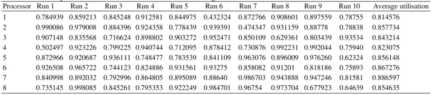
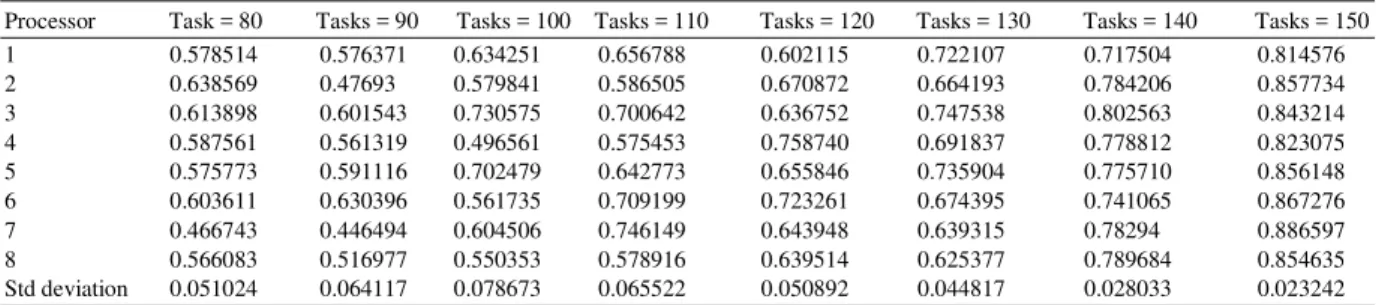
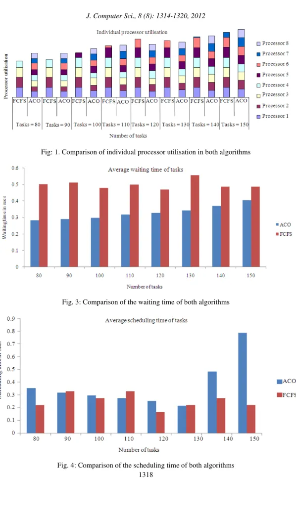
Table 2 and 3 indicate the individual processor utilisation obtained for ten trial runs for tasks sets of size 80 and 150 respectively. Similar results are generated for the other tasks sets but are not shown here. The average utilisation of each of the eight processors using ACO is shown in Table 4, for all problem instances. Table 5 shows the same for the FCFS algorithm. Figure 1 pictorially depicts this fact. Table 6 shows the average waiting time of all the tasks and Table 7 the average time taken for generating the schedule using ACO for all the eight problem instances. Table 8 gives a comparison of the two parameters, average waiting time and scheduling time of both the algorithms. Figure 3 and 4 pictorially represent the average waiting time and average scheduling time of the tasks using ACO and FCFS algorithms respectively.

Table 2: Individual processor utilisation for a task set of size = 80 using ACO

Processor Run 1 Run 2 Run 3 Run 4 Run 5 Run 6 Run 7 Run 8 Run 9 Run 10 Average utilisation

1 0.656084 0.700213 0.885165 0.406228 0.763305 0.773982 0.298284 0.364099 0.573676 0.3641 0.578514 2 0.582901 0.674038 0.663830 0.842179 0.686192 0.548480 0.466564 0.721615 0.478275 0.72162 0.638569 3 0.395874 0.671931 0.289019 0.695151 0.734577 0.704704 0.824187 0.710339 0.402859 0.71034 0.613898 4 0.670888 0.313425 0.689824 0.590311 0.562306 0.549707 0.705603 0.714157 0.365236 0.71416 0.587561 5 0.428755 0.729906 0.593352 0.659602 0.788282 0.601688 0.669223 0.278909 0.729103 0.27891 0.575773 6 0.417844 0.524486 0.605786 0.644437 0.351635 0.535320 0.653824 0.818237 0.666307 0.81824 0.603611 7 0.742216 0.524340 0.410301 0.466626 0.466619 0.337011 0.466235 0.321595 0.610891 0.32160 0.466743 8 0.688504 0.780932 0.584626 0.367148 0.538258 0.328475 0.513205 0.590841 0.678001 0.59084 0.566083

Table 3: Individual processor utilisation for a task set of size = 150 using ACO

Processor Run 1 Run 2 Run 3 Run 4 Run 5 Run 6 Run 7 Run 8 Run 9 Run 10 Average utilisation

1317 Table 4: Average Processor utilisation for ACO for all 8 problem instances

Processor Task = 80 Tasks = 90 Tasks = 100 Tasks = 110 Tasks = 120 Tasks = 130 Tasks = 140 Tasks = 150

1 0.578514 0.576371 0.634251 0.656788 0.602115 0.722107 0.717504 0.814576

2 0.638569 0.47693 0.579841 0.586505 0.670872 0.664193 0.784206 0.857734

3 0.613898 0.601543 0.730575 0.700642 0.636752 0.747538 0.802563 0.843214

4 0.587561 0.561319 0.496561 0.575453 0.758740 0.691837 0.778812 0.823075

5 0.575773 0.591116 0.702479 0.642773 0.655846 0.735904 0.775710 0.856148

6 0.603611 0.630396 0.561735 0.709199 0.723261 0.674395 0.741065 0.867276

7 0.466743 0.446494 0.604506 0.746149 0.643948 0.639315 0.78294 0.886597

8 0.566083 0.516977 0.550353 0.578916 0.639514 0.625377 0.789684 0.854635

Std deviation 0.051024 0.064117 0.078673 0.065522 0.050892 0.044817 0.028033 0.023242

Table 5: Processor utilisation table for FCFS for all 8 problem instances

Processor Task = 80 Tasks = 90 Tasks = 100 Tasks = 110 Tasks = 120 Tasks = 130 Tasks = 140 Tasks = 150

1 0.999868 0.997173 0.998363 0.999082 0.999750 0.999876 0.998197 0.999695

2 0.993046 0.996016 0.998884 0.999709 0.999904 0.999869 0.999198 0.999930

3 0.997989 0.997549 0.999344 0.999262 0.998091 0.999686 0.998984 0.999368

4 0.638526 0.792437 0.996648 0.998617 0.996428 0.991380 0.999906 0.998867

5 0.000000 0.000000 0.465335 0.987451 0.998315 0.999198 0.997494 0.997635

6 0.000000 0.000000 0.000000 0.206958 0.802481 0.657856 0.977435 0.996723

7 0.000000 0.000000 0.000000 0.000000 0.000000 0.000000 0.092169 0.524179

8 0.000000 0.000000 0.000000 0.000000 0.000000 0.000000 0.000000 0.000000

Std deviation 0.498996 0.509959 0.495432 0.484447 0.452179 0.451279 0.440108 0.368644

Table 6: Average waiting time of all the tasks for ACO for all the 8 problem instances

Waiting time

Tasks Run 1 Run 2 Run 3 Run 4 Run 5 Run 6 Run 7 Run 8 Run 9 Run 10 (sec) Average

80 0.272352 0.298573 0.306115 0.283122 0.269575 0.284789 0.272519 0.290696 0.265357 0.29070 0.283379 90 0.23708 0.261958 0.275055 0.250937 0.278498 0.310585 0.471085 0.276304 0.263216 0.28554 0.291026 100 0.280952 0.321592 0.28699 0.289454 0.332356 0.276751 0.287561 0.327144 0.288574 0.28454 0.297592 110 0.336543 0.364722 0.321728 0.284489 0.316022 0.32348 0.340149 0.290859 0.302946 0.31270 0.319363 120 0.284736 0.304845 0.368304 0.363478 0.345521 0.310871 0.299553 0.330165 0.335844 0.35510 0.329842 130 0.369743 0.315029 0.360452 0.341435 0.366506 0.327045 0.351238 0.320950 0.348863 0.33560 0.343686 140 0.393407 0.34719 0.354999 0.377763 0.382686 0.363617 0.350132 0.419890 0.391613 0.32555 0.370685 150 0.399324 0.421531 0.391251 0.418564 0.400483 0.415324 0.417409 0.418305 0.420223 0.36060 0.406301

Table 7: Average time to generate a schedule using ACO for all the 8 problem instances

Scheduling time

Tasks Run 1 Run 2 Run 3 Run 4 Run 5 Run 6 Run 7 Run 8 Run 9 Run 10 (sec) Average

80 0.549451 0.329670 0.329670 0.219780 0.384615 0.274725 0.329670 0.384615 0.32967 0.384620 0.351648 90 0.384615 0.549451 0.329670 0.274725 0.274725 0.274725 0.219780 0.274725 0.274725 0.329670 0.318681 100 0.439560 0.219780 0.274725 0.274725 0.439560 0.219780 0.274725 0.274725 0.274725 0.274725 0.296703 110 0.274725 0.219780 0.219780 0.219780 0.549451 0.274725 0.274725 0.219780 0.274725 0.219780 0.274725 120 0.274725 0.274725 0.274725 0.384615 0.219780 0.219780 0.219780 0.219780 0.219780 0.219780 0.252747 130 0.219780 0.274725 0.274725 0.219780 0.219780 0.164835 0.164835 0.219780 0.219780 0.164835 0.214286 140 0.439560 0.329670 1.923077 0.439560 0.329670 0.329670 0.274725 0.329670 0.219780 0.219780 0.483516 150 0.549451 0.439560 1.648352 0.329670 0.989011 0.494505 1.703297 0.824176 0.549451 0.329670 0.785714

Table 8: Comparison of the waiting time and the scheduling time of both algorithms

Average waiting time of tasks (sec) Average scheduling time of tasks (sec)

--- ---

Tasks ACO FCFS ACO FCFS

80 0.283379 0.503323 0.351648 0.219780

90 0.291026 0.513061 0.318681 0.329670

100 0.297592 0.479564 0.296703 0.274725

110 0.319363 0.501489 0.274725 0.329670

120 0.329842 0.471085 0.252747 0.164835

130 0.343686 0.557086 0.214286 0.219780

140 0.370685 0.488277 0.483516 0.274725

1318

Fig: 1. Comparison of individual processor utilisation in both algorithms

Fig. 3: Comparison of the waiting time of both algorithms

1319

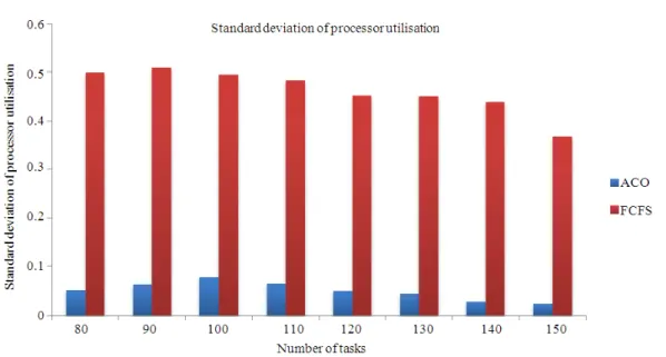
Fig. 2: The comparison of the standard deviation of the utilisation of all the processors using the two algorithms

DISCUSSION

It is seen from Table 5 that the number of processors not utilised by the FCFS scheduling algorithm varies from 1 to 4. But all the processors are utilised by the ACO algorithm as shown in Table 4. The last row of Table 4 and Table 5 give the standard deviation of the utilisation across all the 8 processors for the respective algorithms. Figure 2 shows the comparison of the standard deviation of the utilisation of all the processors using the two algorithms. This substantiates our claim that the load is fairly shared among all the processors in ACO. It is shown from Figure 3 that the average waiting time for the tasks is more in the case of FCFS compare to ACO. There is however a marginal increase in the scheduling time in case of ACO wih respect to FCFS as shown in Figure 4.

CONCLUSION

A different approach to task scheduling on heterogeneous processors based on ACO is presented. Our approach attempts to find a feasible task assignment with the objective of keeping all the processors more or less equally loaded. On comparison with the FCFS approach, the ACO method balances the load fairly among the different processors. The average waiting time of the tasks is also found to be less than that of FCFS algorithm. But there is a slight increase in the scheduling time for the ACO algorithm.

REFERENCES

Blum, C. and A. Roli, 2003. Metaheuristics in combinatorial optimization: Overview and conceptual comparison. ACM Comput. Surv. 35: 268-308. DOI: 10.1145/937503.937505

Blum, C., 2005. Ant colony optimization: Introduction and recent trends. Phys. Life Rev., 2: 353-373. DOI: 10.1016/j.plrev.2005.10.001

Braun, D.T., H.J. Siegel, N. Beck, L.L. Boloni and M. Maheswaran et al., 2001. A comparison of eleven static heuristics for mapping a class of independent tasks onto heterogeneous distributed computing systems. J. Parallel Distributed Comput., 61: 810-837. DOI: 10.1006/jpdc.2000.1714

Chen, H. and A.M.K. Cheng, 2005. Applying ant colony optimization to the partitioned scheduling problem for heterogeneous multiprocessors. ACM USA., 2: 11-14. DOI: 10.1145/1121788.1121793 Chen, H., A.M.K. Cheng and Y.W. Kuo, 2011.

Assigning real-time tasks to heterogeneous processors by applying ant colony optimization. J. Parallel Distributed Comput., 71: 132-142. DOI: 10.1016/j.jpdc.2010.09.011

1320 Radulescu, A. and V.J.C. Gemund, 2002. Low-cost task

scheduling for distributed-memory machines. IEEE Trans. Parallel Distributed Syst., 13: 648-658. DOI: 10.1109/TPDS.2002.1011417

Shih-Tang, L., C. Ruey-Maw, H. Yueh-Min and W. Chung-Lun, 2008. Multiprocessor system scheduling with precedence and resource constraints using an enhanced ant colony system. Expert Syst. Appli., 34: 2071-2081. DOI: 10.1016/j.eswa.2007.02.022

Srikanth, G.U., V.U. Maheswari, A.P. Shanthi and A. Siromoney, 2012. A survey on real time task scheduling.Eur. J. Sci. Res., 69: 33-41.