Solving the Travelling
Salesman Problem Using the
Ant Colony Optimization
Ivan Brezina Jr. Zuzana Čičková
Article Info:
Management Information Systems, Vol. 6 (2011), No. 4, pp. 010-014
Received 12 July 2010 Accepted 23 September 2011
UDC 005.658.6
Summary
In this article, we study a possibility of solving the well-known Travelling Salesman Problem (TSP), which ranges among NP-hard problems, and offer a theoretical overview of some methods used for solving this problem. We discuss the Ant Colony Optimization (ACO), which belongs to the group of evolutionary techniques and presents the approach used in the application of ACO to the TSP. We study the impact of some control parameters by implementing this algorithm. The quality of the solution is compared with the optimal solution.
Keywords
travelling salesman problem, met heuristics, ant colony optimization
1. Introduction
Travelling salesman problem (TSP) consists of finding the shortest route in complete weighted graph G with n nodes and n(n-1) edges, so that the start node and the end node are identical and all other nodes in this tour are visited exactly once. The most popular practical application of TSP are: regular distribution of goods or resources, finding of the shortest of costumer servicing route, planning bus lines etc., but also in the areas that have nothing to do with travel routes. We will mention some of them as an illustration:
Drilling holes for electrical circuits for flat machines;
Starlight interferometer satellite positioning;
Applications in crystallography;
Chain diagram optimization;
Computer motherboard components layout;
Industrial robot control;
2. Problem Formulation
Let C be the matrix of shortest distances
(dimension nxn), where n is the number of nodes of graph G. The elements of matrix C represents
the shortest distances between all pairs of nodes (i, j), i, j=1, 2, …,n. The travelling salesman problem can be formulated in the category programming binary, where variables are equal to 0 or 1, depending on the fact whether the route from node I to node j is realized (xij= 1) or not (xit= 0).
Then, the mathematical formulation of TSP (Brezina, 2003) is as follows (the idea of this formulation is to assign the numbers 1 through n
to the nodes with the extra variables ui, so that this
numbering corresponds to the order of the nodes
in the tour. It is obvious that this excludes sub-tours, as a sub-tour excluding the node 1 cannot have a feasible assignment of the corresponding ui
variables):
1 1
min n n
ij ij i j
c x
(1)subject to
1
1 n
ij i
x
j1, 2,...ni
j
(2)1
1 n
ij j
x
i1, 2,...ni
j
(3)1 i j ij
u u nx n i j, 2, 3,...n i j (4)
0,1ij
x i j, 1, 2,...n
i
j
(5)3. Solving the Travelling Salesman Problem (TSP)
The Travelling Salesman Problem is one of the best known NP-hard problems, which means that there is no exact algorithm to solve it in polynomial time. The minimal expected time to obtain optimal solution is exponential. So, for that reason, we usually use heuristics to help us to obtain a “good” solution. Many algorithms were applied to solve TSP with more or less success. There are various ways to classify algorithms, each with its own merits. The basic characteristic is the ability to reach optimal solution: exact algorithms or heuristics.
well only for solving the problems with no more than 40-80 nodes (we suppose the use of one computer). For the practical relevance, it is necessary to solve the larger-scale problems with the help of heuristics. Heuristic methods vary from exacts methods in that they give no guarantee to find the optimal solution to the given problem (so that solution is called suboptimal), but in many cases this is the solution of good quality and we can obtain it in acceptable time. Heuristic methods are usually focused on solving the special type of problems.
The significant part of heuristics comprises metaheuristic methods, which differs from the classical methods in that they combined the stochastic and deterministic composition. It means that they are focused on global optimization, not only for local extremes. The big advantage of met heuristics is that they are built not only for solving a concrete type of problem, but they describe general algorithm in that, they show only the way, how to apply some procedures to become solution of the problem. This procedure is defined only descriptively, by black-box, and the implementation depends from the specific type of problem. The group of the most known met heuristics includes evolutionary algorithms, which are inspired by process in nature (for example genetic algorithms, particle swarm optimization, differential evolution, ant colony optimization, etc.).
4. Ant Colony Optimization for Solving the Travelling Salesman Problem
Ant colony optimization (ACO) belongs to the group of metaheuristic methods. The idea was published in the early 90s for the first time. The base of ACO is to simulate the real behaviour of ants in nature. The functioning of an ant colony provides indirect communication with the help pheromones, which ants excrete. Pheromones are chemical substances which attract other ants searching for food. The attractiveness of a given path depends on the quantity of pheromones that the ant feels. Pheromones excretion is governed by some rules and has not always the same intensity. The quantity of pheromones depends on the attractiveness of the route. The use of more attractive route ensures that the ant exudes more pheromones on its way back and so that path is more also attractive for other ants. The important characteristic of pheromones is evaporation. This process depends on the time. When the way is no
longer used, pheromones are more evaporated and the ants begin to use other paths.
What is important for ACO algorithm the moving of ants. This motion is not deterministic, but it has stochastic character, so the ants can find the path, which is firstly unfavourable, but which is ultimately preferable for food search. The important characteristic is that a few individuals continuously use non-preferred path and look for another best way.
ACO was formulated based on experiments with double path model, where the quantification was made similar to Monte Carlo method. The base of this simulation was two artificial connections between the anthill and a food source. The simulation demonstrated that ants are able to find the shorter these two paths. A significant impact of this simulation was to quantify the behaviour of ants.
For practical use of ACO, it was necessary to project virtual ants. It was important to set their properties. These properties help virtual ants to scan the graph and find the shortest tour. Virtual ants do not move continuously; they move in jumps, which means that, after a time unit, they will always be in another graph node. The absolved path is saved in ant memory. The created cycles are detected in ant memory. In the next tour, the ant decides on the base of pheromones power. Just because the property of pheromone evaporation, pheromones on shortest edges are stronger, because of the fact that the ant goes across these edges faster.
Based on these facts we can mathematically describe the behaviour of the virtual ants (Onwubolu & Babu, 2004, p. 712):
4.1. Design of the Solution
Moving of virtual ant depends on the amount of pheromone on the graph edges. The probability pik
of transition of a virtual ant from the node i to the node k is given by formula (6). We assume the existence of internal ant’s memory.
∑ (6)
where
τi - indicates the attractiveness of transition in
the past
ηi - adds to transition attractiveness for ants, Ni - set of nodes connected to point i, without
the last visited point before i,
4.2. Reverse
Virtual ant is using the same reverse path as the path to the food resource based on his internal memory, but in opposite order and without cycles, which are eliminated. After elimination of the cycles, the ant puts the pheromone on the edges of reverse path according to formula (7).
t t ij t
ij
1 (7) where
τijt- value of pheromone in step t,
Δτ- value by ants saved pheromones in step t. Values Δτ can be constant or they can be changed depends of solution quality.
4.3. Evaporation of Pheromones
At last, the pheromones on the edges are evaporated. The evaporation helps to find the shortest path and provide that no other path will be assessed as the shortest. This evaporation of pheromones has an intensity ρ (8).
tij t
ij
1 1(8) This formula is applied on all graph edges with intensity ρ (interval (0, 1)).
On this knowledge we can compose an algorithm of ACO, which can be used for solving the travelling salesman problem. It is necessary to keep information about quantity of pheromones τij
in memory, which has stochastic character and actually represents state of graph scan. Further on, there is a need to memorize the edge costs, or information derived from this information (ηij).
Information of pheromones value τij is changing
during the simulation, but values of ηij stay the
same during the calculation. Virtual ants use this information during their moving across the graph. On the basis of these considerations, we can describe the ACO algorithm as system of steps (Chu, 2009, p. 107):
1. Ants scan graph G. The aim of this scan is to find an optimal solution
2. Every ant has its own memory, which is used for saving information about travelled path (for example about travelled nodes). This memory can also serve to ensure constraints or to evaluate of the solution.
3. The process begins in state xsk and has one or
more ending constraints ek. Let the actual state
of an ant be the state xr = (xr–1, i) and no
ending constraint is complied, so the ant moves to node j in neighbourhood of the state Nk(xr)
and the ant moves to the new state (xr, j) X.
In case that some ending constraint is complied
with, the ant ends with process of scan. The transition to a state that represents unacceptable solution is usually banned by appropriate implementation of internal ant memory.
4. The next ant motion depends on the probability, which is calculated on the base of pheromone quantity on edges of graph, and it also takes into consideration its local memory and the acceptance of this step.
5. If the ant can to add new component of graph
GC, it can update the value of corresponding
pheromone information (information is bound with corresponding edge, or aim node).
6. The ant can update pheromone values after reverse path construction by editing associate pheromone values.
5. Computational Experiments
The moving of ants provides the parallel and independent search of the route with the help of dynamical change of pheromone trail. The ant represents an elementary unit with the ability to learn, and due to collective-cooperative work with other members of population, it is able to find acceptable solution to the given problem.
For experiment, we used the problem of 32 cities in Slovakia. We were able to get an optimal solution to that problem with the help of GAMS (Solver Cplex, 17498 iterations, optimal length of route 1453 km). Secondly, we try to solve that problem using ACO algorithm (6 functions in Matlab _information, Ants_primaryplacing, Ants_cycle, Ants_cost, Ants_traceupdatin and script Main (MATLAB, 2007).
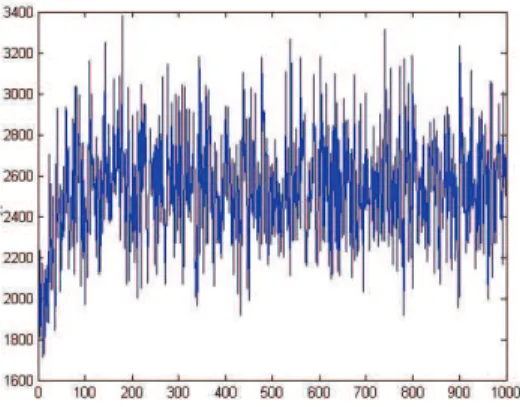
Chu (2009) recommends parameters = 1, =5. The number of iterations was set to 1000 (iter=1000) simultaneously with the changing number of ants (m = 100, 1000, 5000, 10000) scanning the graph the number of ants (m) were changed as well.
Figure 1 Running of simulation for m=100
Subsequent simulations were realized with
m=1000. The result was the tour with length
k=1621 in 34th iteration (difference 11.56% from optimal route). The running of search is shown in Figure 2.
Figure 2 Running of simulation for m=1000
Further on, we set the number of ants to 5000 (m=5000). Algorithm ACO finds the tour with length k=1532 in 21st iteration (difference 5.44% from optimal route). The searching process is shown in Figure 3.
Figure 3 Running of simulation for m=5000
At last, the number of ants was set to 10000 (m=10000). Algorithm ACO find the tour with length k=1465 in 242nd iteration, (deviation from optimal solution was 0.83%). The progress of searching (route length decreasing) is shown in Figure 4.
Figure 4 Running of simulation for m=10000
6. Conclusion
Based on the experiments, it can be concluded that the quality of solutions depends on the number of ants. The lower number of ants allows the individual to change the path much faster. The higher number of ants in population causes the higher accumulation of pheromone on edges, and thus an individual keeps the path with higher concentration of pheromone with a high probability. The final result differs from optimal solution by 12 km (deviation is less than 0-9 %). The great advantage over the use of exact methods is that ACO algorithm provides relatively good results by a comparatively low number of iterations, and is therefore able to find an acceptable solution in a comparatively short time, so it is useable for solving problems occurring in practical applications.
The results of simulations are summarized in Table 1.
Table 1 Summary of results of ACO simulations
Parameter Iter m k l
1000 100 1713 10
1000 1000 1612 34 1000 5000 1532 21
References
Brezina, I. (2003). Kvantitatívne metódy v logistike. Bratislava: Ekonóm. Chu, A. (2009). Metaheuristická metóda mravčej kolónie pri riešení
kombinatorických optimalizačných úloh. Praha: Vysoká škola ekonomická v
Praze.
MATLAB. (2007, May 21). Solving tsp with ant colony system. Retrieved October 12, 2009, from The MathWorks:
http://www.mathworks.com/matlabcentral/fileexchange/15049
Onwubolu, G. C., & Babu, B. V. (2004). New Optimization Techniques in
Engineering. Berlin-Heidelberg: Springer-Verlag.
Ivan Brezina Jr.
University of Economics in Bratislava Faculty of Economic Informatics
Department of Operations Research and Econometrics Dolnozemská cesta 1/b
852 35 Bratislava Slovakia
Email: [email protected]
Zuzana Čičková
University of Economics in Bratislava Faculty of Economic Informatics
Department of Operations Research and Econometrics Dolnozemská cesta 1/b
852 35 Bratislava Slovakia