www.nonlin-processes-geophys.net/15/783/2008/ © Author(s) 2008. This work is distributed under the Creative Commons Attribution 3.0 License.
Nonlinear Processes
in Geophysics
Solute transport in fractured media – analysis of non-reversibility in
tracer tests
N. E. V. Rodrigues1, J. L. M. P. de Lima2, and F. F. Cruz3
1Earth Sciences Department, Faculdade de Ciˆencias e Tecnologia da Universidade de Coimbra, Largo Marquˆes de Pombal,
3000-272 Coimbra, Portugal
2Civil Engineering Department, Faculdade de Ciˆencias e Tecnologia da Universidade de Coimbra, Rua Lu´ıs Reis Santos –
P´olo II Universidade de Coimbra, 3030-788 Coimbra, Portugal
3Civil Engineering Department, Escola Superior de Tecnologia e Gest˜ao de Leiria, Morro do Lena – Alto do Vieiro, 2411-901
Leiria, Portugal
Received: 11 December 2007 – Revised: 3 September 2008 – Accepted: 3 September 2008 – Published: 23 October 2008
Abstract. This paper describes several small-scale (lab-oratory) experiments designed to simulate solute transport through fractured formations. A block of granite was bro-ken to produce a fracture similar to those found in natural environments. Seven holes were drilled in the block to in-tersect the fracture. Later these holes functioned as either inlet or outlet points. All the possible combinations of pairs of inlet-outlet points were used to set up the tracer tests that provided the data analysed in this paper.
The results indicate that reverse tracer tests do not neces-sarily provide symmetric results. Under some circumstances, the non-reversibility might be used to detect differences in the morphology of the fracture. The results also indicate that it is possible to estimate reasonably well the volume avail-able for the circulation of the fluid by using transport models that neglect diffusion.
1 Introduction
It is important to study solute transport in fractured forma-tions because the fractures can create conduits which become fast flow paths for the circulation of fluids and/or dissolved species. Fractured formations represent a large portion of the solid Earth. For instance, in Portugal, they cover about two thirds of the surface of the country. Even those formations that are considered porous media are affected by faulting, and the distribution of flow is far from uniform. Applications for accurate tests can be found, for instance, in the following ar-eas: oil fields (e.g. Zemel, 1995), hydrogeology (e.g. Bear et
Correspondence to:N. E. V. Rodrigues ([email protected])
al., 1993; K¨ass, 1998; Hill and Tiedman, 2007), radioactive waste disposal (e.g. Gylling et al., 1998). The simplifica-tions that have been introduced give rise to inaccuracies that are not usually taken into account.
784 N. E. V. Rodrigues et al.: Solute transport in fractured media
−
Fig. 1. Set-up of the laboratory experiments (adapted from Cruz, 2000).
fits into the context of the second question, focusing on solute transport. The propagation rate (Rodrigues, 1994) of solute transport is a fast process (e.g. Novakowski et al., 2004).
Current modelling of solute transport in fractured media is a two-step procedure: (1) resolution of the flow problem, and (2) resolution of the transport problem (e.g. Bear and Verruijt, 1987; Hill and Tiedman, 2007). The flow problem supplies medium flow velocity values for the transport prob-lem. Analytical and numerical solutions exist for a number of cases (recent attempts can be found, for instance, in Chen et al., 2007; Novakowski and Bogan, 1999; Carlier et al., 2006; Coronado and Ram´ırez-Sabag, 2005). These methods can lead to wrong estimates because the distribution of velocities can create flow paths very different from those foreseen by the modelling (Rodrigues, 1994).
The initial aim of this work was the evaluation of proce-dures for the calculation of the volume available for the cir-culation of the fluids in fractured media. However the exper-iments raised difficulties like the non-uniqueness of answers for similar flow conditions, and so some of the questions and proposed explanations are shared in this paper.
In the laboratory, an artificial fracture in a granite block was intersected by several holes. Several tracer tests were then conducted. The tests intended to: (i) analyse the ad-vection and dispersion of solutes in fractured media and (ii) assess the importance of the velocity field in the dispersion of solutes in fractured media.
2 Experimental procedure and set-up
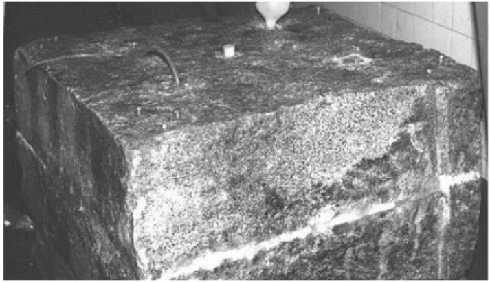
One granite block was used for the laboratory tests. The block came from a quarry which is located about 100 km north-east of Coimbra (Portugal). The quarry site is domi-nated by late Hercynian granite (Geological Map of Portugal, Sheet 17-C, scale 1:50000). This rock is porphyritic granite, grey with no preferential orientation of the feldspathic phe-nocrysts. This is a light-coloured rock with 10–15% mafic minerals.
Fig. 2.Granite block and detail of the sealed fracture.
The block was split longitudinally in order to create an ar-tificial fracture (Figs. 1 and 2) that was later used as the flow path of the water. The sides of the fracture were sealed with a silicone sealant, to guarantee that all the water circulated inside the block and to prevent possible leaks.
Tap water was used in the tests and some of its character-istics are given in Table 1.
The block of granite used in the laboratory tests measured approximately 1 m×1 m×0.60 m. The artificial horizontal fracture was intersected by seven vertical holes, 0.025 m in diameter (Figs. 1 and 2).
During each test a constant flow of water was injected in one of the holes and extracted from another, while all the oth-ers were kept shut. An injection-extraction pair of wells was simulated in each case. The measured volume corresponding to two holes plus the fracture was 2.6 litres.
At the beginning of each test, small amounts of soluble chemicals were injected into the water (pulse injection) and from that moment on (initial time, t0)the variation of the
concentration of the solute in the outlet hole was registered. The tests were organized in two groups: (i) using the com-binations of five holes (A, B, C, D, and E, respectively, centre and vertices of a square) and (ii) a dipole with two holes (des-ignated “X” and “Y”). With this framework it was possible to plan 22 (twenty-two) different configurations (A (in) to B (out), B to A, . . . , E to D, X to Y and Y to X). As three chemical solutes were used in the tracer tests (sodium chlo-ride, sulphorhodamine and uranine), a total of 66 (sixty-six) tracer tests were carried out. Table 2 summarizes the general conditions of the tests.
On average each test lasted one hour. It was observed that most of injected tracer left the system within thirty minutes. The temperature of the water and the pH remained constant for the duration of the tests (around 18◦C and pH of 6.8).
Table 1.Characteristics of the water used in the experiments (SMASC, 2001).
Temperature Conductivity pH Cl SO4 NH4 (◦C) (µS cm−1) (–) (mg L−1) (mg L−1) (mg L−1)
18 107 7.0 12.5 10.9 0.032
NO3 NO2 HCO3 Na Ca K Fe Zn
(mg L−1) (mg L−1) (mg L−1) (mg L−1) (mg L−1) (mg L−1) (µg L−1) (µg L−1)
3.8 0.003 27.6 10.3 7.9 1.3 70 140
Table 2.General conditions of the tracer tests.
Tracer Concentration(g/L) Amount injected (ml) Mean flow rate (L/s)
Sodium chloride 250 10 0.0167
Sulphorhodamine 0.0001 10 0.0167
Uranine 0.0001 10 0.0167
The concentrations of sulphorhodamine and uranine (sodium fluorescein) were measured with a portable fluo-rimeter. This device recorded the measurements on a disk and they were later transferred to a computer. The software converts the measured fluorescence values into concentra-tion values. The system was able to record two simultaneous tracer tests.
3 Methodology
The tests involved the continuous injection of water through the fractured block of granite. The flow rate and the temper-ature were kept constant during each tracer test.
It is useful to recall the notion of characteristic time,tc(s),
the time necessary for some transport phenomena to propa-gate a certain distanceL(m), which applies to diffusion type equations with the parameters adapted to each case (e.g. Ro-drigues, 1994):
tc= L2
4D (1)
whereD (m2/s) is the diffusivity coefficient of the specific phenomena.
The rock matrix is, for practical purposes, impermeable in relation to fluid flow, taking into account the presence of a rather more permeable joint. For the tracer tests the diffusiv-ity coefficient is a diffusivdiffusiv-ity of momentum and consequently it is given byvL∗ (whereV is the fluid flow velocity (m/s)
andL∗is a characteristic length). In this case the character-istic time is of the order of a couple of minutes.
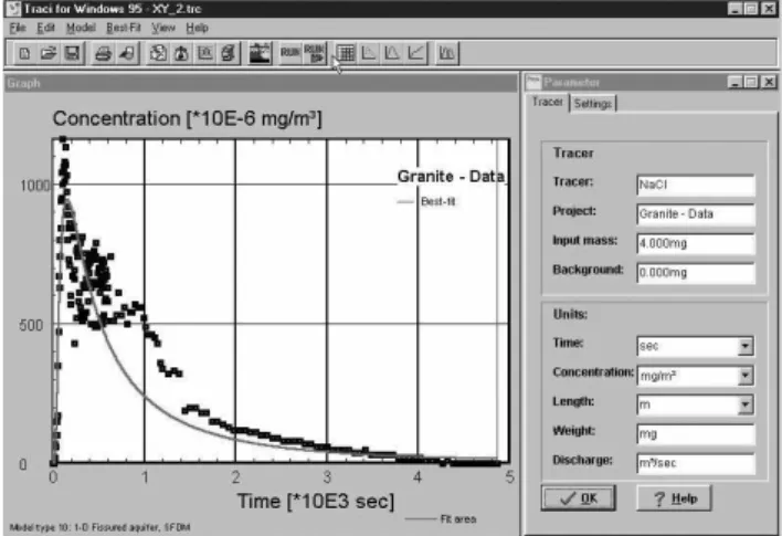
Fig. 3.Example of a tracer test (X to Y) and the best fit curve from Traci95.
By recording the concentration of the solutes (in the cases of uranine and sulphorhodamine) or the conductivity of the water (in the case of sodium chloride) it was possible to cal-culate the moments of the tracer test curves or the parameters of the “Single Fissure Dispersion Model” (SFDM) developed by Maloszewski and implemented in the software Traci95 (K¨ass, 1998). Figure 3 below shows the screen output of one of the interpreted results obtained with this software.
outlined in Appendix A. Further details are available in the literature (e.g., K¨ass, 1998; Bear and Verruijt, 1987; Leven-spiel, 1972; Cook, 2003).
In this study two different approaches have been used to estimate system parameters. One is probabilistic and it is based on the characterisation of the probability density func-tions of the residence times (e.g. Levenspiel, 1972). The sec-ond approach is deterministic. First a geometric model of the system is assumed. Then the flow problem followed by the transport problem are solved (e.g. Bear and Verruijt, 1987).
The residence time distribution function,f (t )dt, (Leven-spiel, 1972) represents the probability that a particle picked at random has a time of residence inside the system between
tandt+dt. This can be expressed as:
f (t )dt= ∞ C(t )
R
0
C(t′) dt′
dt= Q
MC(t )dt (2)
where f (t ) is the density function of the residence time
(s−1); C(t )is the mass concentration measured at the exit
(kg/m3);Qrepresents the flow rate (m3/s) andMis the mass of tracer injected “instantaneously” (kg).
Recalling that in the tests with sodium chloride the electri-cal conductivity was measured instead of the concentration and knowing that the relation between conductivity and con-centration is linear:
C(t )=K Cv(t ) (3)
where C(t ) is the sodium chloride mass concentration (kg/m3),Cv(t )is the conductivity (S),Kis a proportionality
constant (kg/m3/S), andtis the time (s).
Substituting in (2) the relationship (3) we obtain:
f (t ) dt = ∞K Cv(t ) dt
R
0
K Cv(t′) dt′
= ∞Cv(t ) dt
R
0
Cv(t′) dt′
(4)
It should be pointed out that the concentration and conductiv-ity values used in the equations above are corrected values: in the concentration case the values do not take into account the initial background concentration, and in the conductivity case the values do not take into account the initial conductiv-ity of the water. This means that:
Cv(t )=Cvmeasured(t )−Cvwater(t ) (5)
In the data processing it was assumed that the conductivity of the water remained constant and that it was equal to the value read at the beginning of each test before the injection of the sodium chloride.
Finally for the numerical calculation off (t )dt a simple discretization has been used:
f (tj)=
Cv(t )
∞
R
0
Cv(t′) dt′
∼
= n Cv(tj)
P
i=1
Cv(ti) 1ti
(6)
with1ti=ti−ti−1andt0=beginning of the test andtn=time
at the end of the test.
¯
t =
∞
Z
0
t f (t ) dt ∼=
n P
j=1
tjCv(tj) 1tj
n P
i=1
Cv(ti) 1ti
(7)
where,t¯is the mean time and
Vf =Qt¯ (8)
is the “volume of fluid circulation”.
Dispersion parameters were not calculated using this ap-proach because they would be moments of order two of the density function (variance or standard deviation) and they would not have an obvious physical meaning (i.e. they would not be directly related to physical characteristics of the flow). Assuming a deterministic model, the data were processed with the software “Traci95” (K¨ass, 1998). It implements the SFDM model (“Single Fissure Dispersion Model– simula-tion of the transport through a fractured system with the pos-sibility of diffusion into the solid matrix). This model was developed by Maloszewski (K¨ass, 1998). In the software the functionf (t )assumes the role of a normalized concentration function, resulting from an injection of a mass of tracer given by:
M= 1
Q
∞
R
0
C(t ) dt
(9)
whereQis the flow rate (m3/s),Mis the mass of the injected
tracer (kg).
The program allows the experimental data to be adjusted to the model. The adjustment parameters are: the mean time, the Peclet number and a parameter,a1, which is defined as:
a= np
p
Dp
2b (10)
where 2bis the fracture aperture (m),npis the porosity of the
solid matrix (m3/m3)andDp is the coefficient of diffusion
(m2/s). This parameter describes the diffusion process for the solid.
As usual, the Peclet number is defined asP e=LV
D , where Lis some characteristic length, which, in the current context, represents the shortest distance between the injection and the extraction holes (m); V is the average velocity of the flow
(m/s); andDis the coefficient of molecular diffusion (m2/s). High Peclet numbers represent solute transport dominated by advection, while low Peclet numbers correspond to transport where molecular diffusion dominates.
1Symbolsa,bandn
pof this equation correspond to the
Table 3.Tracer tests in the dipole X and Y.
Sodium Chloride
X→Y Y→X Delta
Mean time (s)∗ 1142 82 1.732 Mean time (s)∗∗ 994 251 1.194 Mean Volume (l)∗ 17.8 1.2 1.747 Mean Volume (l)∗∗ 15.5 3.7 1.229 Peclet Number 0.6 8.8 –1.745
Fluorescein Sulphorhodamine
X→Y Y→X Delta X→Y Y→X Delta
Mean time (s)∗ 92 62 0.390 78 63 0.213
Mean time (s)∗∗ 292 286 0.021 250 218 0.137
Mean Volume (l)∗ 1.5 1.0 0.400 1.5 1.4 0.069
Mean Volume (l)∗∗ 4.9 4.8 0.021 4.2 3.6 0.154
Peclet Number 18.2 19.2 –0.053 12.2 1.6 1.536
∗– Values obtained from the output of Traci95.
∗∗– Values calculated using Eqs. 7 (mean time) or 8 (mean
volume).
4 Results and discussion
First it is convenient to visualize the general framework. What we have here is a set up made of a fracture plus a set of holes that provide the points into and out of the system. The volume available for the fluid flow is known. When a test is carried out two holes are open and all the others are shut so the volume is at the most 2.6 litres (fracture plus two holes). In chemical engineering this is also usually the case: the vol-ume of the chemical reactor is known and so is the mean time. However this is not the usual case in geosciences: the volume of the system and the mean time are the main param-eters being sought. So we were able to test the interpretations that are made with the models in current use and that have been described in the previous section.
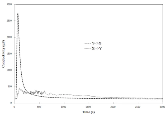
The results for the dipole X and Y are summarized in Ta-ble 3 and Fig. 4 below. TaTa-ble 3 shows the calculated param-eters for the tracer testes that have used the holes “X” and “Y”. A parameter (Delta) has been devised for the purpose of comparing reverse tracer tests:
Delta=[(H1→H2)−(H2→H1)]/0.5×[(H1→H2)+(H2→H1)]
where H1→H2 (H2→H1) represent the parameters calcu-lated when the fluid flows from hole H1 to hole H2 (or from hole H2 to hole H1). The parameter Delta provides a mea-sure of the deviation from symmetrical results (if the tests where symmetrical thenDelta=0).
The most noticeable aspect of the results is the difference between the tests with sodium chloride and the tests with flu-orescein or sulphorhodamine. Also remarkable is the differ-ence between (X→Y) tests and (Y→X) tests, especially in
Fig. 4.Reverse tracer tests with noticeably different shapes.
the sodium chloride tests (Fig. 4). The most probable rea-son in both cases is the fact that the sodium chloride solution injected had a higher density than the water. As a result, if there are significant openings near the injection hole then the solution might sink there initially. It will be released later as it diffuses into the flowing water. If there are no pits near the injection point then the solution gets mixed with the flowing water more easily and so it travels faster through the system. The results show that there were some pits next to hole “X”, acting as initial receivers of the heavier sodium chloride solu-tion. Thus, one conclusion is that the transport might depend on the morphology of the areas around the injection holes, and the residence time of the sodium chloride molecules will be proportional to openings next to these areas. Therefore, the parameters calculated in the tests with sodium chloride do not correspond to the parameters of the flowing water.
For the remaining tests, the calculated results are synthe-sised in Fig. 5. In the figure there are pairs of values. The first value represents the volume, in litres, estimated from the parameters of the Traci95 simulation output and the sec-ond values (in brackets) represents the volume estimated af-ter Eq. 8 (for instance, for the pair E (inlet) and D (outlet) the estimated volumes where 0.9 litres and 6.7 litres). It is quite clear that all flow paths are different, thus highlighting the non-reversibility of these processes.
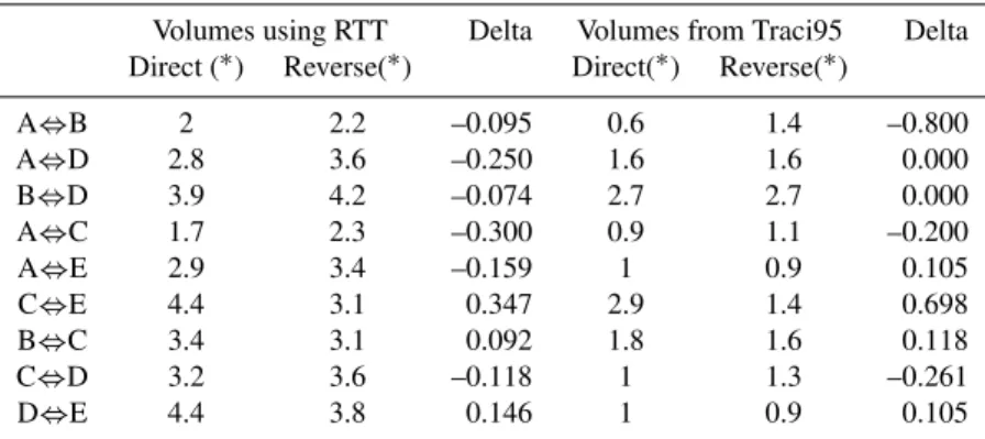
Parameters characterizing the flow pattern without being affected by exogenous factors can be obtained from the tests with fluorescein or sulphorhodamine because they behave as inert tracers (e.g. K¨ass, 1998; Rodrigues, 1994). In addition to values from Tables 3, 4a and b give the calculated volumes for each pair of reverse tracer tests, using either the residence time theory (RTT, Eq. 8) or Traci95.
−
Fig. 5.Tests with NaCl – Volumes (l) from Traci95 and Eq. (8) (in brackets).
measured by thedeltaparameter, may be a order of magni-tude different. Even the results from the mathematical model (used by Traci95), which are less affected by the tail of the tracer curve (unlike the RTT results), show consistent dif-ferences. This indicates that the flow paths in reverse tracer tests are not necessarily the same, and that the existing mod-els are unable to simulate this non-reversibility. Comparing the shapes of the tracer curves it becomes clear that the dif-ferences are most significant in the tails of the reverse tracer tests. This fact is amplified if the data are plotted in a semi-logarithmic graph. An example of tests using sulphorho-damine in holes A and B is shown in Fig. 6.
The volumes calculated in the tests (using Eq. 8) with fluorescein and sulphorhodamine varied between 1.7 and 4.9 litres. About eighty percent of the values, calculated us-ing the residence time theory, were greater than 2.6 litres (the correct measured volume). This overvaluing of the calcu-lated volumes is due, in principle, to the effects of molec-ular diffusion from areas of low flow, resulting in particles with very long residence times distorting the calculation of the mean residence times.
If we consider the results from Traci95, the calculated vol-umes vary from 0.6 to 2.9 litres, and only three of them are larger than 2.6 litres. These values are acceptable but it should be kept in mind that the model only explains the initial part of the curve, and it does not consider the values of the tail of the test. Thus in a situation where the volume is not known it is recommended to use Traci95 or some similar program, but keeping in mind that the value is a lower limit because it represents the portion of the total volume open to fluid flow where most of the fluid circulates.
The calculated values using the residence time should be regarded as upper limits and they should be analysed taking into account the possible existence of “dead ends”.
Tests with Sulphorodamine
0.01 0.1 1 10 100 1000 10000
0 200 400 600 800 1000 1200
Time (s)
Conc
ent
ra
tion (
p
pb) A to B
B to A
−
Fig. 6.Reverse tracer tests in holes A and B.
To sum up, the tests with fluorescein and sulphorhodamine confirm that these dye products are inert during the trans-port. Even though the results with sodium chloride were in-fluenced by the density of the ejected fluid, they provided a positive side effect: they can be used to amplify the differ-ences in the circulation between pairs of wells and thus give clues about the morphology of the fractures in the vicinity of the injection wells.
5 Conclusions
These experimental results allow the following conclusions to be drawn:
1. For the tests in the laboratory, the fluorescein and the sulphorhodamine were revealed to be good tracers, and no significant differences were found in the results. As expected, the observed transport was advection (high Peclet numbers). In fast tests, like those performed in the laboratory, the two tracers do not indicate hetero-geneities in the surface of the fractures. Having said that, different results from the tests in pairs of holes have been obtained and the differences are clearer in the tails of the curves.
2. The tests with sodium chloride revealed an interesting side effect: the use of NaCl as a trace can be used to amplify morphological differences in flow paths. The “pulse” of injected sodium chloride might get caught in the bottom of the injection holes and their vicinity due to the higher density. It will be delayed in relation to the flowing water and this will give some indication about the heterogeneities of the fracture surface.
Table 4a.Calculated volumes for the tests with sodium fluorescein.
Volumes using RTT Delta Volumes from Traci95 Delta Direct (∗) Reverse(∗) Direct(∗) Reverse(∗)
A⇔B 2.7 2.5 0.077 0.7 1.1 –0.444
A⇔D 2.9 4.2 –1.115 1.6 1.2 0.286
B⇔D 3.8 4.3 –0.123 1.9 2.2 –0.146
A⇔C 2.1 2.3 –0.091 1 1.1 –0.095
A⇔E 3.6 3.6 0.000 0.8 0.8 0.000
C⇔E 4.6 3.5 0.272 1.8 1.6 0.118
B⇔C 4.0 4.2 –0.049 1.4 1.3 0.074
C⇔D 4.6 4.0 0.140 1.1 1.1 0.000
(∗) – Direct meaning first hole to second hole and Reverse means second hole to first hole; for instance, for A⇔B Direct means injection in A and extraction of the fluid in B.
Table 4b.Calculated volumes for the tests with sulphorhodamine.
Volumes using RTT Delta Volumes from Traci95 Delta Direct (∗) Reverse(∗) Direct(∗) Reverse(∗)
A⇔B 2 2.2 –0.095 0.6 1.4 –0.800
A⇔D 2.8 3.6 –0.250 1.6 1.6 0.000
B⇔D 3.9 4.2 –0.074 2.7 2.7 0.000
A⇔C 1.7 2.3 –0.300 0.9 1.1 –0.200
A⇔E 2.9 3.4 –0.159 1 0.9 0.105
C⇔E 4.4 3.1 0.347 2.9 1.4 0.698
B⇔C 3.4 3.1 0.092 1.8 1.6 0.118
C⇔D 3.2 3.6 –0.118 1 1.3 –0.261
D⇔E 4.4 3.8 0.146 1 0.9 0.105
(∗) – Direct meaning first hole to second hole and Reverse means second hole to first hole; for instance, for A⇔B Direct means injection in A and extraction of the fluid in B.
disregarding places where there is slow fluid circulation. The use of models based on residence time theory will give upper limits.
4. For the set up that has been used here it was expected that reverse tracers tests would provide similar results. However, reverse tracer tests can differ from one an-other quite a lot. The existing models cannot explain all the relevant features of the fluid flow.
Appendix A
Solute transport and the advection-dispersion equation
The advection-dispersion equation has been used to describe the transport of material in solution at a microscopic level (e.g. Bear and Verruijt, 1987):
∂c
∂t = −∇ ·(cV−D∇c)+ρŴ (A1)
whereC(t )is the mass concentration, V is the velocity of the fluid (vector),Dis the coefficient of molecular diffusion (tensor),ρis the density of the fluid andŴis the rate at which
the mass of material is added to (or removed from) the fluid. This equation states that the concentration of solute at a point varies as a result of (i) transport by the fluid (C(t )v) (a linear process) and (ii) differences in concentration between points(D.∇C(t )), a non-linear process). The last term (ρŴ)
denotes the change in concentration due to chemical reac-tions or decay phenomena.
Analytical solutions exist only for a limited number of simplified cases (e.g. K¨ass, 1998) Most of the solutions are for the one-dimensional (1-D) flow with no chemical reac-tion. In this case the equation reduces to:
∂C
∂t =D
∂2C
∂x2 −V
∂C
∂x (A2)
790 N. E. V. Rodrigues et al.: Solute transport in fractured media
Fig. A1.Channel with wings (Rodrigues, 1994).
The complex geometry of porous media prevents the use of these equations. The definition of averaged variables (ve-locity and concentration) over a small portion of the porous media (“representative elementary volume” – REV) is one of the methods proposed to break this impasse (Bear and Ver-ruijt, 1987). The total flux of solute through a porous medium is expressed as (Bear and Verruijt, 1987):
qc,total=ω(CV−Dh· ∇C) (A3)
whereqc,totalis the total flux of solute by advection,
disper-sion and diffudisper-sion,ωis the kinematic porosity,Cis the aver-age concentration,V is the pore water velocity,Dh=D+D∗
is the coefficient of hydrodynamic dispersion (second order rank symmetrical tensor),Dis the coefficient of molecular diffusion in a porous medium (second order rank tensor),D∗
is the coefficient of mechanical dispersion (second order rank tensor).
The main effect of the averaging process is the introduc-tion of an addiintroduc-tional dispersive term. Three mechanisms cause this dispersion: (i) velocity variations across the pores; (ii) velocity variations between pores; (iii) differences in streamline path length.
For a macroscopic balance of solute transport, Eq. (A2) becomes (Bear and Verruijt, 1987):
∂ωC
∂t =−∇(Cu−ωD·∇C−ωD
∗·∇
C)−f+ωρŴ−P C+RCr (A4)
whereωC is the mass of solute per unit volume of porous medium,uis the seepage or Darcy’s velocity,f is the quan-tity of solute that leaves the fluid as a result of ion exchange and adsorption,P is the pumping rate flow (per unit volume of porous medium per unit time),Ris the recharge rate flow (per unit volume of porous medium per unit time) andCr is
the concentration of added fluid. Other terms have the same meaning as before.
With no interaction with the solid matrix, no decay and no pumping or recharge of fluid, Eq. (A4) simplifies to:
∂C
∂t = ∇(Dh· ∇C−vC) (A5)
whereV=u/ω is the pore water velocity, C=concentration
of solute in the fluid and Dh=coefficient of hydrodynamic
dispersion.
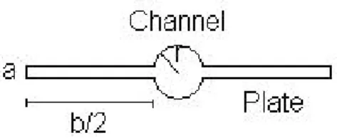
Equation (A5) is the one normally adopted in studies of so-lute transport through porous media. In the case of fractured media there is a combination of several effects; the most im-portant of which is the fact that the fluid flow is controlled by channelling. This means that most of the flow occurs in a number of dendritic pathways in the fracture surface, with average apertures greater than the average aperture of the fracture. The volume of the channels represents a small fraction of the total volume open to flow. A simplified model can be used to show that most of the fluid flows through a small percentage of the volume available for the flow. The model is a combination of a parallel plate with a pipe, re-ferred to below as a “channel with wings” (Fig. A1, adapted from Rodrigues, 1994).
The formulas, that describe the fluid flow between smooth parallel plates and in smooth pipes assuming Poiseuille flow, are used in the calculations below.
The distribution of flow mentioned (10% of the fracture’s volume open to fluid flow is swept along by more than 80% of the fluid) is used to constrain the volumes of the plate and of the pipe. The volume of the pipe is assumed to be 10 times smaller than the volume of the plate. In the calculations the radius of pipe,r, is 10 times the aperture of the plate,a
(assume 100µm and 10µm, respectively).
The calculated velocity of the fluid flowing through the pipe is 150 times larger than the velocity of the fluid caught in the plate for the same hydraulic gradient and viscosity of the fluid:
upipe
uplate
=150 (A6)
whereurepresents the velocity of the fluid in the pipe or in the plate.
So a particle of tracer travelling in the plate is, on average, 150 times slower than one circulating through the pipe. The ratio between flow rates is:
Qpipe
Qplate
=15 (A7)
i.e. through a volume which is 10 times smaller flows 15 times more fluid.
The value of the breadth of the plate is b∼=3 cm or
b/2=1.5 cm each side of the pipe, which is a physically ac-ceptable figure.
The volume associated with regions of slow-moving fluid (“the wings”) can be an order of magnitude larger than the volume of the “channels” but most of the fluid flows through the “channels” even though they have a much smaller volume than the plates.
Acknowledgements. Fundac¸˜ao para a Ciˆencia e Tecnologia (Por-tuguese Foundation for Science and Technology) provided financial support through the Project PTDC/ECM/70456/2006.
of the University of Coimbra. The support from the Department of Earth Sciences of the University of Coimbra and IMAR – Institute of Marine Research is also acknowledged.
The comments of the anonymous reviewers helped to improve significantly this paper. Their effort is commended.
Edited by: A. Tarquis
Reviewed by: four anonymous referees
References
Bear, J. and Verruijt, A.: Modeling Groundwater Flow and Pollu-tion, D. Reidel Pub. Comp., Dordrecht, The Netherlands, 1987. Bear, J., Tsang, C. F., and de Marsily, G.: Flow and Contaminant
Transport in Fractured Rock, Academic Press, New York, 1993. Carlier, E., El Khattabi, J., and Potdevin, J. L.: Solute transport in sand and chalk: a probabilistic approach, Hydrological Pro-cesses, John Wiley & Sons, 20, 1047–1055, 2006.
Chen, J. S., Chen, C. S., and Chen, C. Y.: Analysis of solute trans-port in a divergent flow tracer test with scale-dependent disper-sion, Hydrological Processes, John Wiley & Sons, 21, 2526– 2536, 2007.
Cook, P. G.: A guide to regional groundwater flow in fractured rock aquifers, CSIRO, Australia, 2003.
Coronado, M. and Ram´ırez-Sabag, J.: A New Analytical Formula-tion for Interwell Finite-Step Tracer InjecFormula-tion Tests in Reservoirs, Transport in Porous Media, Springer, 60, 339–351, 2005. Cruz, F. F.: Dispers˜ao de Contaminantes em Meios Fracturados
– Ensaios Experimentais com Trac¸adores. (Contaminant disper-sion in fractured media – Experimental tests with tracers), M. Sc. Thesis, Faculty of Science and Technology of the Coimbra University, Portugal, 2000 (in Portuguese).
Gylling, B., Birgersson, L., Moreno, L., and Neretnieks, I.: Anal-ysis of a long-term pumping and tracer test using the channel network model, J. Contam. Hydrol., 32, 203–222, 1998. Hill M. C. and Tiedman C. R.: Effective Groundwater Model
Cali-bration, John Wiley, 2007.
K¨ass, W.: Tracing Technique in Geohydrology, Taylor & Francis Ltd, Rotterdam, The Netherlands, 1998.
Lee, C.-H. and Farmer, I.: Fluid Flow in Discontinuous Rocks, Chapman & Hall, London, UK, 1993.
Levenspiel O.: Chemical Reaction Engineering, 2nd edition, John Wiley & Sons., New York, USA, 1972.
Louis, C.: Introduction `a l’hydraulique des roches (Introduction to rock hydraulics). Bulletin Bureau de Recherches G´eologiques et Mini`eres 1974; III-4: 283–356, 1974.
Montazer, P.: Monitoring hydrologic conditions in the vadose zone in fractured rocks, Yucca Mountain, Nevada, in: Flow and Trans-port through Unsaturated Fractured Rock, edited by: Evans, D. D. and Nicholson, T. J., Geophys. Monogr. Ser., Vol. 42, 1st ed., AGU, Washington, D. C., 31–42, 1987.
Novakowski, K. S. and Bogan, J. D. A.: Semi-analytical model for the simulation of solute transport in a network of fractures hav-ing random orientations, International Journal for Numerical and Analytical Methods in Geomechanics, John Wiley & Sons, 23, 317–333, 1999.
Novakowski, K. S., Bickerton, G., and Lapcevic, P.: Interpretation of injection-withdrawal tracer experiments conducted between two wells in a large single fracture, Jo. Contam. Hydrol., Else-vier, 73, 227–247, 2004.
NRC: Committee on Fracture Characterization and Fluid Flow, Na-tional Research Council, Rock Fractures and Fluid Flow – Con-temporary Understanding and Applications, National Academy Press, Washington, D.C., USA, 1996.
Rasmussen, T. C. and Evans D. D.: Unsaturated flow and transport through fractured rock related to high-level waste repositories. Tech. Rep. NUREG/CR-4655, US Nucl. Reg. Comm., Washing-ton, D.C., 1987.
Rodrigues, N.: The Interpretation of Tracer Curves in Hot Dry Rock Geothermal Reservoirs. Ph.D. Thesis, Exeter University, UK, 1994.
SMASC: Boletim peri´odico n.◦ S17/01, Laborat´orio Controlo Qualidade dos Servic¸os Municipalizados de ´Agua e Saneamento de Coimbra (SMASC), Coimbra, Portugal, 2001 (in Portuguese). Snow, D. T.: Anisotropic permeability of fractured media, Water
Resour. Res., 5(6), 1273–1289, 1969.