Guia para a formatação de teses Versão 4.0 Janeiro 2006
Watershed-scale runoff routing and solute transport
in a spatially aggregated hydrological framework
MASTERS PROGRAM IN GEOSPATIAL TECHNOLOGIES
Watershed-scale runoff routing and solute
transport in a spatially aggregated hydrological
framework
Master thesis
by
Jairo Arturo Torres Matallana
Institute for Geoinformatics, ifgi,
Westf¨
alische Wilhelms-Universit¨
at, M¨
unster, Germany
Instituto Superior de Estat´ıstica e Gest˜
ao de Informa¸c˜
ao, ISEGI,
Universidade NOVA de Lisboa, Portugal
Deptartamento de Lenguajes y Sistemas Informaticos, LSI,
Universitat Jaume I, Castell´
on, Spain
Watershed-scale runoff routing and solute transport in a
spatially aggregated hydrological framework
Dissertation
Supervised by
Prof. Dr. Edzer Pebesma
ifgi - Institute for Geoinformatics
Westf¨
alische Wilhelms-Universit¨
at
M¨
unster, Germany
Co-supervised by
Dra. Ana Cristina Costa
ISEGI - Instituto Superior de Estat´ıstica e Gest˜
ao de Informa¸c˜
ao
Universidade NOVA de Lisboa
Lisboa, Portugal
Co-supervised by
Dr. Jorge Mateu
LSI - Departamento Lenguajes y Sistemas Informaticos
Universitat Jaume I
Disclaimer
Author’s Declaration
I hereby declare that this Master thesis has been written independently by me, solely based on the specified literature and resources. All ideas that have been adopted directly or indirectly from other works are denoted appropriately. The thesis has not been submitted for any other examination purposes in its present or a similar form and was not yet published in any other way.
Signature: ...
Acknowledgments
The author expresses acknowledgment to the Consortium of Universities: the Institute for Geoinformatics, ifgi, of the University of M¨unster, the Instituto Su-perior de Estat´ıstica e Gest˜ao de Informa¸c˜ao, ISEGI, of the Universidade Nova de Lisboa and the Departmento de Lenguajes y Sistemas Informaticos, LSI, of the Universitat Jaume I, Castell´on, Spain, for all the high quality academic support.
Also, the author gives his acknowledgment to the Consortium of Universities and the European Comission for its financial support through the Scholarship Erasmus Mundus.
The author gives a special acknowledgment to professor Edzer Pebesma, principal advisor of the present document, for his total support both academic and personal, and for motivating the author for developing R code and to go beyond and search for challenging ideas.
Also, the author gives his acknowledgment to the professors in the first semester developed at ISEGI, specially to professors Marco Painho, Cristina Costa, Pedro Cabral and Roberto Henriques, for all his academic and personal support. Also, the administrative personal deserves a kind acknowledgment.
In the same way, the author gives his acknowledgment to the professors in the second semester developed at ifgi, specially to professors Christoph Brox, Werner Kuhn and Pedro Ribeiro, for all his academic and personal support. Also, the Committee of the Graduate School and the administrative personal deserves a kind acknowledgment.
The author gives special attention to the medical body of the Santa Maria Hospital in Lisbon and the Uniklinikum in M¨unster for all the medical support along finishing the studies.
To my loved wife, Paola
and
Abstract
This document presents the implementation of several methods for geo-spatial analysis of river networks and watersheds for runoff routing and solute trans-port in Rin order to contribute in a comprehensive hydrological modelling to the current framework of theRpackage ”hydromad”.
The main aim of the study is to developRroutines to coupled the outputs of the hydrological framework of theRpackage ”hydromad” to the selected solute transport model looking forward better simulation of water-quality determinants transport at watershed scale.
Following the research scheme presented in this proposal it is possible to prove the hypothesis behind the study. The simulation of solute transport at specific places of the river network was improved by implementing a runoff routing method at watershed-scale, the ”hydromad” package, and by coupling it into a suitable modeling framework for representing solute transport processes. The developed package, ”watersheds”, allows geo-spatial river network anal-ysis and makes use of the Catchments and Rivers Network System (ECRINS) version 1.1, which constitutes the hydrographical system currently in use at the European Environment Agency as well as widely serving as the reference sys-tem for the Water Information Syssys-tem for Europe (WISE). The versatility of the code generated lets to implement geo-spatial analysis in any watershed included into the ECRINS, as a consequence, watersheds along entire Europe could be analyzed. This constitutes an important fact because several institutions or scientific community related with the WISE system could take advantage of the package and this document.
Keywords
Contents
1 Introduction 1
1.1 Justification . . . 1
1.2 Hypothesis . . . 2
1.3 Objectives . . . 2
2 Literature review 2 2.1 Hydrological modelling. . . 2
2.1.1 Soil Moisture Accounting models . . . 3
2.1.2 Routing models. . . 4
2.1.3 Calibration methods . . . 5
2.2 Geo-spatial and Geo-temporal capabilities . . . 5
2.2.1 sp . . . 5
2.2.2 rgeos . . . 5
2.2.3 rgdal . . . 6
2.2.4 maptools . . . 6
2.2.5 raster . . . 6
2.2.6 lattice . . . 6
2.2.7 multicore . . . 6
2.2.8 Watersheds . . . 7
2.3 Runoff routing and solute transport . . . 7
2.3.1 General reaction transport equation in 1-Dimension . . . 7
2.3.2 Boundary conditions in 1-D models. . . 8
2.3.3 Numerical approximation of the Advection Dispersion Equa-tion . . . 9
2.3.4 1-D finite difference grids and properties in ReacTran . . 9
2.3.5 Stability . . . 10
2.4 RPackages for routing and solute transport modelling . . . 11
2.4.1 ReacTran . . . 11
2.4.2 deSolve . . . 12
2.4.3 rootSolve . . . 12
3 Materials and methods 12 3.1 Datasets . . . 12
3.1.1 The ECRINS dataset . . . 12
3.1.2 Water quality determinants . . . 12
3.1.3 River discharge stations . . . 13
3.1.4 Further datasets available . . . 13
3.2 Methodology . . . 14
3.3 Site study: river Weser basin, Germany . . . 17
3.3.1 Subsets . . . 17
4 Results 19 4.1 Geo-spatial analysis of zhyd subbasins . . . 19
4.1.1 TheWatershedsobject . . . 23
4.1.2 TheWatersheds.Ordermethod . . . 25
4.1.3 TheWatersheds.Order2method . . . 26
4.1.4 TheWatersheds.IOR1function . . . 27
4.1.6 TheWatersheds.IOR3function . . . 29
4.1.7 TheWatersheds.IOR4function . . . 30
4.1.8 The Karlshafen and Wahmbeck Stations watersheds . . . 31
4.2 Precipitation time series management . . . 32
4.3 Flow time series management . . . 33
4.4 Runoff routing and hydrological modelling . . . 34
4.5 Routing and solute transport modelling . . . 36
5 Conclusions 40 6 Further work 41 References 42 7 Appendices 44 7.1 TheWatersheds.Ordermethod . . . 44
7.2 TheWatersheds.Order2method . . . 46
7.3 TheWatersheds.IOR1function . . . 49
7.4 TheWatersheds.IOR2function . . . 51
7.5 TheWatersheds.IOR3function . . . 53
7.6 TheWatersheds.IOR4function . . . 55
7.7 The Karlshafen and Whambeck Stations watersheds . . . 57
7.8 Precipitation time series management . . . 60
7.9 Routing and solute transport modelling . . . 62
List of Figures
1 The modelling framework in the hydromad package. . . 3
2 Overview of thehydromadpackage. . . 4
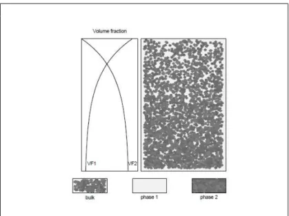
3 An illustration of multiple phases in ReacTran. From Soetaert and Meysman (2012), Figure 1 . . . 8
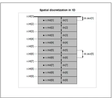
4 Spatial 1-D discretization in ReacTran. From Soetaert and Meysman (2012), Figure 2. . . 10
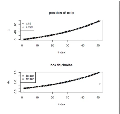
5 Exponential grid cell size in ReacTran. From Soetaert and Meysman (2012), Figure 3. . . 11
6 Flow and level stations on river Weser . . . 14
7 Flow and level stations at Germany available in the BfG portal . 15 8 River Rhein level at K¨oeln station . . . 15
9 River Rhein level at D¨usseldorf station . . . 16
10 Strahler stream order. Illustration. . . 16
11 River Weser basin . . . 19
12 River Weser subbasin and tributaries . . . 20
13 River Weser and intersecting zhyd subbasins. . . 20
14 River Weser and all zhyd subbasins . . . 21
15 River Weser and river network . . . 21
16 River Weser and all zhyd subbasins . . . 22
17 Flow chart of the Watersheds package. Red=data input; blue rectangle = process; green rectangle = algorithm; diamond shape = decision. . . 24
18 Current zhyd watershed (1) and first order tributary watersheds (1.1 , 1.2) . . . 26
19 Current zhyd watershed and 1st and 2nd order tributary watersheds 27 20 Spatial analysis of watershed outlet, case I . . . 28
21 Spatial analysis of watershed outlet, case II . . . 29
22 Spatial analysis of watershed inlet and outlet, case III . . . 30
23 Spatial analysis of watershed inlet and outlet, case IV . . . 31
24 The Karlshafen and Wahmbeck Stations watersheds . . . 32
25 Precipitation time series at Wahmbeck Station . . . 33
26 Precipitation time series at Wahmbeck Station . . . 34
27 Modelled and observed streamflow time series . . . 35
28 Flow chart of the hydrological modelling. Red=data input; blue rectangle = process; green rectangle = algorithm . . . 36
29 Simulation time series of OC and flow between the Wahmbeck and Kalshafen stations on 01.01.1995 . . . 37
30 Simulation time series of OC and flow between the Wahmbeck and Kalshafen stations on 02.01.1995 . . . 38
31 Simulation time series of OC and flow between the Wahmbeck and Kalshafen stations on 03.01.1995 . . . 38
32 Simulation time series of OC and flow between the Wahmbeck and Kalshafen stations on 04.01.1995 . . . 39
33 Simulation time series of OC and flow between the Wahmbeck and Kalshafen stations on 05.01.1995 . . . 39
List of Tables
1 Flow and level measurement stations, river Weser. . . 13
2 Parameter definition . . . 35
3 Parameter calibration results . . . 35
List of Acronyms
AWBM: Australian Water Balance Model
BfG: Federal Institute of Hydrology, Germany
CCM: Catchment Characterisation and Modelling
CMD: Catchment Moisture Deficit
CORINE: Coordination of Information on the Environment
CWI: Catchment Wetness Index
ECRINS: Catchments and Rivers Network System
ECA&D: European Climate Assessment & Dataset
EEA: European Environment Agency
EOBS: Observational dataset for precipitation, temperature and sea level pressure in Europe
FEC: Functional Elementary Catchment
HEC-HMS: Hydrologic Engineering Center - Hydrological Modeling Sys-tem
IHACRES: Identification of unit Hydrographs And Component flows from Rainfall, Evaporation and Streamflow
LISFLOOD: GIS-based hydrological rainfall-runoff-routing model
NetCDF: network Common Data Form
SMA: Soil Moisture Accounting
SWAT: Soil Water Assessment Tool Model
USACE: United States Army Corps of Engineers.
USGS: United States Geological Survey
WATFLOOD: Integrated set of computer programs to forecast flood flows
WaSiM: Water balance Simulation Model
WFD: Water Framework Directive
WISE: Water Information System for Europe
1 Introduction
In a comprehensive environmental modelling in the water resources domain, is of paramount importance to understand the interaction between the mate-rial flows to coastal waters that are constrained by catchment boundaries and the human activities therein, and those materials that are tied to trade and other trans-boundary processes (e.g. residence time, transport and fate of phys-ical, chemical and microbiological water-quality determinants) and their global implications on preserving the quality of the natural environment.
In a similar sense, applications in river and environmental engineering, specif-ically related with hydrological modelling, are related to the analysis of rainfall and hydrometric time series in order to implement rainfall-runoff models as a conceptual mathematical basis in flood risk management e.g. the study of the probable maximum precipitation and probable maximum flood for basin water resources management. In this case, the modelling framework is for creating the conceptual basis to simulate flood events in probable scenarios of storm events. The present document has the purpose of illustrating the implementation of the spatial analysis and the runoff routing and solute transport in the framework of the ECRINS river network a reference system for hydrological and climate change modelling in order to contribute in a comprehensive modelling framework by means of the understanding and representation of the flow celerities dynamics and spatial distribution in the river network at the watershed scale.
In the following sections are presented the justification of the proposal (Sec-tion 1.1), the hypothesis behind the study (Section 1.2) and the objectives (Section 1.3). Also, in the Section 2, the preliminary review of literature is introduced; the software and datasets required, and the methods to follow are presented in Section 3. The Section 4 presents the results of the study. The conclusions (Section 5) and some considerations for further work are presented (Section6). Finally, references and appendices (Section7) are presented.
1.1 Justification
The ultimate aim of flow prediction using models must be to improve deci-sion making e.g. in water resources planning, flood protection and mitigation of contamination (K. J. Beven,2012). From the Millenium Development Goals (MDGs) point of view (United Nations - UN,2012), to secure water-quality and predict floods have an impact on reducing child mortality (Goal 4) and ensure environmental sustainability (Goal 7). Currently, UN (2012) also recognizes that improving monitoring systems is paramount due to reliable, timely and internationally comparable data on the MDG indicators are crucial for devis-ing appropriate policies and interventions needed to achieve the MDGs and for holding the international community to account. In this sense, rainfall-runoff models are a primary component in the monitoring system for real-time flow and water-quality prediction.
In the literature exists several hydrological models for rainfall-runoff mod-elling. However, there are few studies that attempt to model both flow and water-quality in a totally consistent way because before is required to represent adequately the complexity of the system e.g. the dynamics of celerities and the complete distribution of water pore velocities (K. J. Beven,2012). Some studies that points toward this direction are provided byBotter et al.(2009,2010) and
Moreover, for addressing a comprehensive hydrological modelling, specifi-cally looking forward on the validation of the hydrological cycle, and the trans-port and fate of sediments and solutes in surface water resources, it is paramount to recognize that in environmental modelling all model structures, regardless of their complexity, are to some extent in error (K. J. Beven,1989;Grayson et al.,
1992;Freer et al.,2004).
Therefore, model comparison in structure, calibration methods and simu-lation events, is essential for choosing objectively the suitable configuration of the model for addressing a specific task related with hydrological modelling. To accomplish this, a novel, versatile, and open source application is provided with the R Project for Statistical Computing (Ihaka & Gentleman, 1996; R Development Core Team,2013). Rmore than a statistical software is a model-ing framework that provides for standardised tests and comparisons of models. Also, theRenvironment allows the reproducibility of methods and results, as is often required by science and research.
The implementation of a method for runoff routing in the river network contributes to the existing hydrological modelling framework and intends for the representation of the solute transport in the river network at the watershed-scale domain.
1.2 Hypothesis
The simulation of solute transport at specific places of the river network (measurement stations) could be improved by implementing a runoff routing method at watershed-scale and by coupling it into a suitable modeling frame-work for representing transport processes.
1.3 Objectives
• Primary objective
– To coupled the selected runoff routing model to Rfor representing solute transport in the river network at the watershed-scale domain.
• Secondary objectives
– To implement several methods for geo-spatial analysis of river net-works inR.
– To implement the selected runoff routing in R.
– To define a simulation configuration for testing.
2 Literature review
2.1 Hydrological modelling
Figure 1: The modelling framework in the hydromad package. FromF. Andrews(2011).
of hydrological models is done as the conceptual basis to simulate flood events in probable scenarios of storm events (Torres & Pebesma, 2013).
Regarding to the challenges for modern hydrological and environmental re-search as it is depicted in current rere-searches –e.g. McDonnell et al. (2010);
Swaney et al. (2011)– is essential to understand and develop a comprehensive modelling framework that includes as an important step the uncertainty anal-ysis in order to identify primary physical controls, and henceforth for coupling, in a most suitable way, inland hydrological models with the coastal system at regional, transboundary and global scales.
Henceforth, in hydrological applications a main aim is to consider a suit-able and reproducible modelling framework that takes into account data input, spatial interpolation, calibration and simulation, and includes geospatial capa-bilities for querying, updating, sharing and visualization of data, methods and results (Torres & Pebesma, 2013). This focus is addressed in the following subsections where is presented in a succinct manner the existing open source softwarehydromadaRpackage for hydrological modelling.
hydromadis an interesting hydrological modelling framework presented by
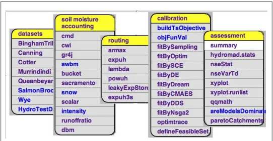
F. T. Andrews, Croke, and Jakeman (2011). The framework is based loosely on the unit hydrograph theory of rainfall-runoff modelling. The documentation of the methods in hydromad could be found in the web page of the project (http://hydromad.catchment.org). The Figure1 illustrates the work-flow of the modelling framework in the hydromad package and the following subsections present a description of the three main components of the hydromad package: the Soil Moisture Accounting (Section2.1.1), the routing models (Section2.1.2) and the calibration methods (Section2.1.3). The Figure2 resumes the compo-nents and structure of the packagehydromad(F. Andrews,2011).
2.1.1 Soil Moisture Accounting models
hydromadcounts with 11 Soil Moisture Accounting (SMA) models (F. Andrews,
Figure 2: Overview of thehydromadpackage. Adapted fromF. Andrews(2014).
the Sacramento Soil Moisture Accounting model. Developed by the US National Weather Service; 7) snow: a simple degree day factor snow model coupled with IHACRES CMD soil moisture model; 8) scalar: a simple constant runoff pro-portion: a constant fraction of rainfall reaches the stream; 9) intensity: Runoff as rainfall to a power. This allows an increasing fraction of runoff to be gener-ated by increasingly intense/large rainfall events (for power >0). The fraction increases up to a full runoff level at maxP; 10) runoffratio: simple time-varying runoff proportion. Rainfall is scaled by the runoff coefficient estimated in a moving window; and 11) dbm: Typical initial model used in Data-Based Mech-anistic modelling. Rainfall is scaled by corresponding streamflow values raised to a power.
The models 10 and 11 use streamflow data, so can not be used for prediction.
2.1.2 Routing models
stores from streamflow.
2.1.3 Calibration methods
Accordingly with F. Andrews(2011), currently implemented calibration meth-ods inhydromadinclude simple sampling schemes (fitBySampling), general op-timisation methods with multistart or presampling (fitByOptim) and the more sophisticated Shuffled Complex Evolution (fitBySCE) and Differential Evolu-tion (fitByDE) methods. All attempt to maximise a given objective funcEvolu-tion. Other 8 calibration algorithms are available (seeF. Andrews(2014)).
Accordingly to F. Andrews (2014) the ”fitBySampling” method fit a hy-dromad model by sampling the parameter space. Returns best result from sampling in parameter ranges using random, latin hypercube sampling, or a uniform grid (all combinations). The function also retains the parameter sets and objective function values, which can be used to define a feasible parame-ter set. The ”fitByOptim” method fits a hydromad model using R’s optim or nlminb functions. Has multi-start and pre-sampling options. The ”fitBySCE” fit a hydromad model using the SCE (Shuffled Complex Evolution) algorithm, and finally, the ”fitByDE” fit a hydromad model using the DE (Differential Evolution) algorithm.
2.2 Geo-spatial and Geo-temporal capabilities
Several packages developed in the programming languageRProject for Sta-tistical Computing (Ihaka & Gentleman, 1996; R Development Core Team,
2013) are available for Geo-spatial and Geo-temporal analysis. The packages sp (Pebesma & Bivand, 2005-2012), rgeos (Bivand & Rundel, 2012), rgdal (Bivand et al., 2003-2013), maptools (Lewin-Koh & Bivand, 2012), raster (Hijmans,2014),Lattice(Sarkar,2012),multicore(Urbanek,2013) andWatersheds was used in the present study and are described in the following subsections.
The present subsection has the purpose of introducing the packages devel-oped in the programming languageRavailable for Geo-spatial and Geo-temporal analysis and used and implemented in the present work.
2.2.1 sp
The packagesp(Pebesma & Bivand,2005-2012), provides classes and methods for spatial data. The classes document where the spatial location information resides, for 2D or 3D data. Utility functions are provided, e.g. for plotting data as maps, spatial selection, as well as methods for retrieving coordinates, for subsetting, print, and summary.
The package has i.a. the class SpatialPolygons which is a data object equivalent to an ESRI polygon shapefile containing information for polygons, and additional similar definitions for spatial points and lines are defined through the objectsSpatialPointsandSpatialLines, respectively.
2.2.2 rgeos
i.a. garea, gBoundary, gBuffer, gCentroid, gContains, gConvexHull, gCrosses, gDifference, gDistance, gEnvelope, gEquals, gIntersection, gIntersects, gRelate, gSimplify, gSymdifference, gTouches, gUnion, SpatialCollections, SpatialRings.
2.2.3 rgdal
A binding package for the Frank Warmerdam’s Geospatial Data Abstraction Library (GDAL, http://www.gdal.org) is available in Rthrough the package rgdal (Bivand et al., 2003-2013). It allows to deploy multiple classes defined in thesppackage and access to the projection/transformation operations from the PROJ.4 library (https://trac.osgeo.org/proj/) and to the OGR library. The OGR Simple Features Library is a C++ open source library for reading, and in some cases writing, a variety of vector file formats including ESRI Shapefiles and PGDBs .mdb files via ODBC (Warmerdam,2013). Therefore, using rgdal both GDAL raster and OGR vector map data can be imported into R and exported, and the ECRINS database could be handled properly.
2.2.4 maptools
The maptools package (Lewin-Koh & Bivand, 2012) is a set of tools for ma-nipulating and reading geographic data, in particular ESRI shape- files; C code used from shapelib. It includes binary access to GSHHS shoreline files. The package also provides interface wrappers for exchanging spatial objects with packages such as PBSmap- ping, spatstat, maps, RArcInfo, Stata tmap, Win-BUGS, Mondrian, and others.
2.2.5 raster
Therasterpackage (Hijmans,2014) has capabilities for reading, writing, ma-nipulating, analyzing and modeling of gridded spatial data. The package im-plements basic and high-level functions and processing of very large files is supported.
2.2.6 lattice
Lattice (Sarkar, 2012), is a powerful and elegant high-level data visualization system, with an emphasis on multivariate data, that is sufficient for typical graphics needs, and is also flexible enough to handle most nonstandard require-ments.
2.2.7 multicore
2.2.8 Watersheds
The package Watershedsdeveloped by the author for the present work, allows spatial analysis for watersheds aggregation and ordering accordingly to an outlet point and size of tributary watershed of the current watershed. Also, enables spatial drainage networks analysis inside the aggregated watersheds. It makes use of the functionalities of the spatial classes, functions and methods of theR packagesp(Pebesma & Bivand,2005-2012). Also is build on the capabilities of theRpackagesrgeos,maptools,lattice,splancs, and multicore.
TheWatershedspackage allows creation and handling of objects class Water-shed for identifying the subbasin that contains the current station (class Spatial- Points) and subsets the zhyd object to subbasin and extract the currentzhyobject that containsstationvia the S4 methodWatershed.Order. Identification of the inlet and outlet stretches and inlet and outlet nodes of the zhyd. Implementation of the functions Watershed.IOR1, .IOR2, .IOR3, and .IOR4 for determining the actual inlet and outlet nodes. S4 methods Watershed.Order2andWatershed.Tributaryfor defining tributary nodes and tributary catchments of the currentzhyd watershed.
2.3 Runoff routing and solute transport
A large-scale runoff routing with an aggregated network-response function is presented by Gong et al.(2009). A scale dependency of routing dynamics is evaluated, as well as the flow velocities and the routing performance at different spatial resolutions. Also, some limitations of aggregated networks are evaluated. An example of runoff routing at large scales that involves development of low-resolution flow networks, with spatial resolutions of which range from 1 Km is presented with the model HYDRO1k (USGS, 1996).
Regarding to identify different schemes of runoff routing in the river network, some distributed and semi-distributed models could be evaluated i. a. WAT-FLOOD (Kouwen, 1988); TOPMODEL (K. Beven et al., 1995; K. J. Beven,
1997; Buytaert, 2012); SASHI (Sistema de An´alise de Simula¸c˜ao Hidrol´ogica, INPE, Renn´o(2003)); SCS-TerraMe (INPE,Pereira (2009)); LISFLOOD (van der Knijff et al., 2010); SWAT (Soil Water Assessment Tool Model, Neitsch et al. (2011)); WaSiM (Water balance Simulation Model, Schulla (2012)); and aggregated models as the Hydrological Modeling System HEC-HMS (USACE, HEC, 2006).
2.3.1 General reaction transport equation in 1-Dimension
Accordingly with Soetaert and Meysman (2012), the general 1-D reaction-transport equation in multi-phase environments and for shapes with variable geometry is:
∂ξC ∂t =−
1 A·
∂(A·J)
∂x +reac (1)
where1
• tis time
Figure 3: An illustration of multiple phases in ReacTran. From Soetaert and Meysman (2012), Figure 1
• xis space
• Cis concentration of a substance in its respective phase
• ξis the volume fraction (-), i.e. the fraction of a phase in the bulk volume (see Figure3). In most of cases, when one phase is consideredξ= 1. For sediments,ξ would be porosity (solutes), or 1-porosity (solids)
• A is the total surface area (L2) • J are fluxes (M L−2t−1)
The Fluxes, J, are estimated per unit of total surface, and represents a dispersive and a advective component:
J=−ξD·∂C
∂x +ξu·C (2)
where:
• Dis the diffusion (or dispersion) coefficient (L2t−1) • uis the advection velocity (Lt−1)
2.3.2 Boundary conditions in 1-D models
Accordingly withSoetaert and Meysman(2012), the boundaries at the extremes of the model domain e.g. atx= 0 could be one of the following options:
• A concentration boundary,C|x=0=C0
• A diffusive + advective flux boundary,Jx=0=J0
2.3.3 Numerical approximation of the Advection Dispersion Equa-tion
Following Soetaert and Meysman (2012), the reaction-transport formula is a partial differential equation (PDE), as a consequence it is solve by approximating the spatial gradients using the numerical differences by the method-of-lines, MOL, approach. This converts the PDE into ordinary differential equations (ODE).
Thus, the model is divided into a number of grid cells, and for each grid cell iis writen:
dξiCi ∂t =−
1 A·
∆i(A·J) ∆xi
+reaci (3)
where ∆i denotes that the flux gradient is to be taken over boxi, and ∆xi is the thickness of the boxi:
∆i(A·J) =Ai,i+1·Ji,i+1−(Ai−1,i·Ji−1,i) (4) wherei, i+ 1 denotes the interface between boxiandi+ 1.
The fluxes at the box interfaces are discretized as:
Ji−1,i=−ξi−1,iDi−1,i·
Ci−Ci−1 ∆xi−1,i
+ξi−1,iui−1,i·(ϑi−1,i·Ci−1+ (1−ϑi−1,i)·Ci) (5) where ∆xi−1,iis the distance between the centre of the grid cellsi−1 and i, and ϑthe upstream weighing coefficients for the advective term.
2.3.4 1-D finite difference grids and properties in ReacTran
the spatial discretization grid could be generated with the functionsetup.grid.1D of the package ReacTran. The generated grid comprises several zones:
setup.grid.1D = function(x.up = 0,x.down = NULL, L = NULL, N = NULL, dx.1 = NULL, p.dx.1 = rep(1,length(L)), max.dx.1 = L,
dx.N = NULL, p.dx.N = rep(1,length(L)), max.dx.N = L)
with the following arguments:
• x.up, the position of the upstream boundary
• x.down, the position of the downstream boundaries in each zone
• L, N, the thickness and the number of grid cells in each zone.
• dx.1, p.dx.1, max.dx.1, the size of the first grid cell, the factor of increase near upstream boundary, and maximal grid cell size in the upstream half of each zone
Figure 4: Spatial 1-D discretization in ReacTran. From Soetaert and Meysman (2012), Figure 2
The function returns an element of classgrid.1Dthat contains the following elements (units L) (see Figure4):
• x.up, x.down, the position of the upstream and downstream boundary
• x.int, the position of the grid cell interfaces, where the fluxes are specified, a vector of length N+1
• x.mid, the position of the grid cell centres, where the concentrations are specified, a vector of length N. This is equivalent to ∆xi−1,i
• dx, the thickness of boxes, i.e. the distance between the grid cell interfaces, a vector of length N. Equivalent to ∆xi
• dx.aux, the distance between the points where the concentrations are spec-ified, a vector of length N+1. This is equivalent to ∆xi−1,i
For example, to represent a subdivision of a river streach of 100 Km long into 50 boxes, with the first box size of 1 Km, is established by:
grid = setup.grid.1D(L=90, dx.1=1, N=50)
and the grid is plotted with the command:
plot(grid)
2.3.5 Stability
Figure 5: Exponential grid cell size in ReacTran. From Soetaert and Meysman (2012), Figure 3
C= ∆t ∆x u
=u∆t
∆x (6)
where:
• Cis the Courant number
• ∆tis the time interval
• ∆xis the space interval
• uis velocity
2.4 R Packages for routing and solute transport modelling
2.4.1 ReacTran
TheRpackage ReacTrancontains routines that enable the development of re-active transport models in aquatic systems (rivers, lakes, oceans), porous media (floc aggregates, sediments,...) and even idealized organisms (spherical cells, cylindrical worms,...) (Soetaert & Meysman,2012).
The geometry of the model domain is either one-dimensional, two-dimensional or three-dimensional. The package contains (Soetaert & Meysman,2012):
• Functions to setup a finite-difference grid (1D or 2D)
• Functions to calculate the advective-diffusive transport term over the grid (1D, 2D, 3D)
2.4.2 deSolve
CitingSoetaert, Petzoldt, and Setzer (2013) from the users manual, the pack-agedeSolve provides ”Functions that solve initial value problems of a system of first-order ordinary differential equations (ODE), of partial differential equa-tions (PDE), of differential algebraic equaequa-tions (DAE), and of delay differential equations. The functions provide an interface to the FORTRAN functions lsoda, lsodar, lsode, lsodes of the ODEPACK collection, to the FORTRAN functions dvode and daspk and a C-implementation of solvers of the Runge-Kutta fam-ily with fixed or variable time steps. The package contains routines designed for solving ODEs resulting from 1-D, 2-D and 3-D partial differential equations (PDE) that have been converted to ODEs by numerical differencing”.
2.4.3 rootSolve
Accordingly Soetaert (2014) from the users manual, the package rootSolve provides ”routines to find the root of nonlinear functions, and to perform steady-state and equilibrium analysis of ordinary differential equations (ODE). Includes routines that: (1) generate gradient and Jacobian matrices (full and banded),(2) find roots of non-linear equations by the Newton-Raphson method,(3) estimate steady-state conditions of a system of (differential) equations in full, banded or sparse form, using the Newton-Raphson method, or by dynamically running, (4) solve the steady-state conditions for uni-and multicomponent 1-D, 2-D, and 3-D partial differential equations, that have been converted to ODEs by numerical differencing (using the method-of-lines approach).”
3 Materials and methods
This section presents a summary of the specific techniques used in the study, procedures, statistical design, and data collection and analysis.
3.1 Datasets
Primary datasets for the present study are defined in the following subsec-tions.
3.1.1 The ECRINS dataset
The European Environment Agency (EAA) has been developed the Catchments and Rivers Network System (ECRINS) version 1.1 (EAA,2012). The ECRINS is the hydrographical system currently in use at the EEA as well as widely serving as the reference system for the Water Information System for Europe (WISE)(EAA, 2012, p. 49).
3.1.2 Water quality determinants
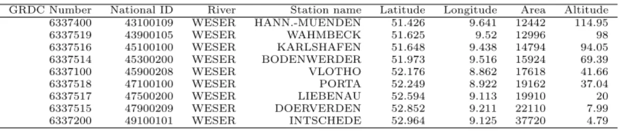
Hy-Table 1: Flow and level measurement stations, river Weser
GRDC Number National ID River Station name Latitude Longitude Area Altitude 6337400 43100109 WESER HANN.-MUENDEN 51.426 9.641 12442 114.95
6337519 43900105 WESER WAHMBECK 51.625 9.52 12996 98
6337516 45100100 WESER KARLSHAFEN 51.648 9.438 14794 94.05
6337514 45300200 WESER BODENWERDER 51.973 9.516 15924 69.39
6337100 45900208 WESER VLOTHO 52.176 8.862 17618 41.66
6337518 47100100 WESER PORTA 52.249 8.922 19162 37.04
6337517 47500200 WESER LIEBENAU 52.594 9.113 19910 20
6337515 47900209 WESER DOERVERDEN 52.852 9.211 22110 7.99
6337200 49100101 WESER INTSCHEDE 52.964 9.125 37720 4.79
drology (BfG):
• water level, cm
• water temperature, degree Celsius
• conductivity,µS/cm
• pH, pH units
• oxygen content, mg/l
• turbidity, TE/F
3.1.3 River discharge stations
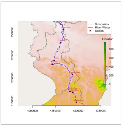
The data for flow level and discharge are also available at Department of Hy-drometry and Hydrological Survey of the German Federal Institute of Hydrol-ogy. The Table1presents the details of the nine stations analyzed in this study and Figure6 shows their location.
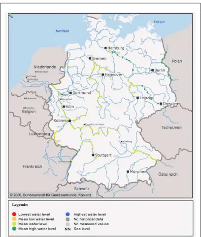
More stations in Germany could be used for implementing the methods for runoff routing and solute transport analysis. Figure 7 presents the available measurement stations in Germany, and Figures 8 and 9 show, as an example, the river Rhein level retrieved at K¨oeln station and D¨usseldorf, respectively.
3.1.4 Further datasets available
• The world-wide repository of river discharge data and associated metadata of theGlobal Runoff Data Centre - GRDC(2013).
• Water levels data at selected gauging stations on German federal water-ways from theGerman Federal Institute of Hydrology - BfG(2013).
• The land cover dataset fromEuropean Environment Agency - EAA(1995). This data project is part of the CORINE programme and is intended to provide consistent localized geographical information on the land cover of the Member States of the European Community.
• Climate data for Germany from the Federal Ministry of Transport, Build-ing and Urban Developmenthttp://www.dwd.de/. From this is created the layer ”dwd PrecipitationStations” and the ODS spreadsheet
0 200 400 600 800
4200000 4250000 4300000 4350000
3150000 3200000 3250000 3300000 HANN.-MUENDEN WAHMBECK KARLSHAFEN BODENWERDER VLOTHO PORTA LIEBENAU DOERVERDEN INTSCHEDE Elevation Sub-basins River Weser Station Sub-basins River Weser Station
Figure 6: Flow and level stations on river Weser
3.2 Methodology
The Catchments and Rivers Network System (ECRINS) version 1.1. from theEAA(2012) is the hydrographical system currently in use at the European level as well as widely serving as the reference system for the Water Information System (WISE).
According with the European Water Framework Directive (WFD), the small-est unitary catchment suggsmall-ested is 10 Km2. The overall aim of ECRINS, how-ever, is to centre the watersheds between 50 km2 and 100 km2, since such a small area is not compatible with production constraints and the source data available. The FEC, or Functional Elementary Catchment, stands as the cen-tral element of ECRINS. FEC refers to the smallest catchment identified as an ECRINS elementary catchment. A FEC is built via aggregating elementary CCM (Catchment Characterisation and Modelling) catchments. It could be ei-ther a ’continental FEC’ when built by aggregating elementary CCM catchments from a non-coastal basin, or a ’coastal FEC’ when elementary CCM catchments belong to a coastal basin (EAA,2012, p. 49).
The average area of possible FEC building from basins at Strahler 3 level is 39 Km2, which is compatible with both this WFD threshold and specific requirements; using basins at level 4 would not allow small enough FECs (EAA,
2012, p. 49). The Figure10presents an illustration of the Stralher stream order 1 to 4.
Figure 7: Flow and level stations at Germany available in the BfG portal
Figure 9: River Rhein level at D¨usseldorf station
Figure 10: Strahler stream order. Illustration.
Personal GeoDatabases (PGDBs) format (a Microsoft�R proprietary format, handed with both MS Access�R and ArcGIS �), is done by using open sourceR GIS methods and database managers. In this sense, R packages as foreign (R Core Team et al., 1999-2013) for importing a .dbf file into a R dataframe, and the S4 methods for manipulating spatial data provided bysp(Pebesma & Bivand,2005-2012) was applied.
The followed methodology was to create a R package (”Waterssheds”) for geospatial analysis of the ECRINS river network for runoff routing and water-shed aggregation based on the order of contribution of tributaries waterwater-sheds (accordingly Strahler order) in the basin of the river Weser, Germany. Although the site of study is defined in the package, it is possible to implement similar analysis for other places contained into the ECRINS dataset (European level).
3.3 Site study: river Weser basin, Germany
The site study is presented along with the package ”Watersheds”. The pack-age has an example dataset of the ECRINS database for the river Weser basin, Germany. The European Environment Agency (EEA) has been developed the Catchments and Rivers Network System (ECRINS) version 1.1. The ECRINS is the hydrographical system currently in use at the European level as well as widely serving as the reference system for the Water Information System (WISE). The current version of ECRINS is based on previous work carried out by the Joint Research Centre (JRC) Catchment Characterisation and Mod-elling (CCM) and the EEA (European Lakes, Dams and Reservoirs Database (Eldred2), European Rivers and Catchments (ERICA), (EAA,2012).
3.3.1 Subsets
The dataset contains the following subsets:
• basin: an objectSpatialPolygonsDataFrameas is defined in packagesp that represents the river Weser basin. Thedata slot contains 6 variables as attributes of 1 observation.
• ctry: an objectSpatialPolygonsDataFrame as is defined in packagesp that represents the administrative boundary of Germany. Thedata slot contains 6 variables as attributes of 1 observation.
• node: an object SpatialPointsDataFrame as is defined in package sp that represents the nodes of the ECRINS river network of the river Weser basin. Thedataslot contains 13 variables as attributes of 3882 observa-tions.
• rAller an object SpatialLinesDataFrame as is defined in package sp that represents the basin of the river Aller, a major tributary of the river Weser. Thedataslot contains 74 variables as attributes of 88 observations.
• rDiemelan object SpatialLinesDataFrame as is defined in package sp that represents the basin of the river Diemel, a major tributary of the river Weser. Thedataslot contains 74 variables as attributes of 39 observations.
• rFulda an object SpatialLinesDataFrame as is defined in package sp that represents the basin of the river Fulda, a major tributary of the river Weser. Thedataslot contains 74 variables as attributes of 82 observations.
• riveran objectSpatialLinesDataFrameas is defined in packagespthat represents the ECRINS river network of the river Weser basin. Thedata slot contains 52 variables as attributes of 3874 observations.
• rWerra an object SpatialLinesDataFrame as is defined in package sp that represents the basin of the river Werra, a major tributary of the river Weser. Thedata slot contains 74 variables as attributes of 120 observa-tions.
• rWeser an object SpatialLinesDataFrame as is defined in package sp that represents the basin of the river Weser. The data slot contains 74 variables as attributes of 104 observations.
• rWiummean object SpatialLinesDataFrame as is defined in package sp that represents the basin of the river Wiumme, a major tributary of the river Weser. Thedataslot contains 74 variables as attributes of 18 obser-vations.
• stationan object SpatialPoints as is defined in packagesp that rep-resents a point of interest for which the watershed will be aggregated an ordered. Could be a point with the coordinates of a measurement station.
• subbasinan objectSpatialPolygonsDataFrameas is defined in package spthat represents the subbasins of the tributaries of the river Weser. The dataslot contains 4 variables as attributes of 4 observations.
• zhyd an object SpatialPolygonsDataFrame as is defined in package sp that contains the primary hydrological units of the river Weser basin ac-cordingly with ECRINS. Thedataslot contains 50 variables as attributes and 915 observations.
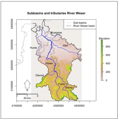
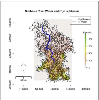
Some examples for visualising the dataset are presented in the following Figures. Figure 11illustrates the River Weser basin location into the German territory. The river Weser is formed after the confluence of the rivers Werra and Fulda. The Figure 12 presents the River Weser subbasin and its main tributaries: the rivers W¨umme, Aller, Hunte and Diemel, and its former rivers Werra and Fulda. The Figure 14 shows the River Weser and its intersecting zhyd subbasins along its trajectory, which represent the primary hydrological units that contribute with the runoff toward the main course.
Figure 11: River Weser basin
outlet nodes of each zhyd and the river network inside them. This is the main effort for developing the package ”Watersheds” a contribution for geo-spatial analysis of the river network of one zhyd unit.
4 Results
This section presents the data acquired for the research and their meaning and analysis. The Section4.1 include some examples for illustrating the capa-bility of geo-spatial analysis in the river network before applying the technique of solute transport in the desired stretch of river. Here are presented the func-tionality of the Watersheds object and the Watersheds.Order method, the Watersheds.Order2 method and the functions Watershed. ,IOR1, IOR2, IOR3,IOR4.
Posteriorly, in Section4.2 is presented the result of the precipitation time series management; in Section4.3is presented the flow time series management; in Section4.4the Runoff routing and hydrological modelling setup is presented; and finally in Section 4.5 are presented the result of applying the numerical approximation of the Advection-Dispersion Equation as the main component of the solute transport modelling.
4.1 Geo-spatial analysis of zhyd subbasins
el-Figure 12: River Weser subbasin and tributaries
Figure 14: River Weser and all zhyd subbasins
Figure 16: River Weser and all zhyd subbasins
ementary catchment. A FEC is built via aggregating elementary CCM (Catch-ment Characterisation and Modelling) catch(Catch-ments. It could be either a ’con-tinental FEC’ when built by aggregating elementary CCM catchments from a non-coastal basin, or a ’coastal FEC’ when elementary CCM catchments be-long to a coastal basin (EAA,2012). The FECs database contains feature class C Zhyd, hereinafter zhyd, which is the most important data set in ECRINS because it constitutes the primary hydrological unit. The structure of zhyd is reported in EAA(2012), Annex 1. This table sets out the FEC IDs (field ZHYD) and all the required IDs of the useful data sets: aggregation water-sheds and reference waterwater-sheds, the connection between FECs and sources of information.
Some examples done via the package ”Watersheds” with the application of the method Watershed.Order and the functionsWatershed. ,IOR1, IOR2, IOR3,IOR4are presented in the next subsections.
Environmental Agency (EAA) and the last one the evaluation of the ”Water-sheds.IOR4” method and the ”stop” node.
After the definition of the ”ECRINS dataset” there are three important task to be developed. These task are the ”identification of the measurement station”, ”the identification of the current zhyd object” and the ”identification of the probable inlet and outlet nodes”, and corresponds to the levels 2 to 4 of the flow chart, respectively.
In the level 5 of the flow chart is created the object ”Watersheds” as is illus-trated in the Section4.1.1. Subsequently, in the level 6 is executed the method ”Watershed.Order” which constitutes the core of the algorithm because through this method are invoked the ”Watersheds. IOR1, IOR2, IOR3 or IOR4” func-tions (level 8 to 11). Each one of these funcfunc-tions constitute a decision node where is checked if the inlet and outlet stretches of the river network inside the current zhyd are of length 1 to 4, respectively. Each one of these functions per-forms the different spatial operations for identifying the inlet and outlet nodes and stretches of river inside and around the current zhyd. Subsequently after the definition of the inlet and outlet object (nodes and stretches of river) in the level 8 right side of the flow chart, is executed the method ”Watershed.tributary”, which performs the spatial operations for identifying the tributary nodes and subsequently the tributary zhyd watersheds of the current zhyd.
Finally after being applied the ”Watershed.Tributary” method, is checked in the level 9, right side of the flow chart, if the object ”Station” from ”Wa-tershed.Tributary” is of length equal to 2, which means that two tributary catchments contributes to the current zhyd watershed. In this positive case is executed the method ”Watershed.Order2” which internally calls the method ”Watershed.Order” for identifying the structure of the inlet and outlet objects (nodes and stretches of river) in each one of the tributary zhyd watersheds. In the negative case, the object ”Station” from ”Watershed.Tributary” is length equal to 1, which mean that just one zhyd watershed is tributary to the current zhyd and as a consequence the method ”Watershed.Order” is invoked again (see right side of the level 9 of the flow chart that return to level 6 ) for determining the inlet and outlet nodes and stretches of river and the river network of this tributary watershed.
In Appendix 7.10 is presented the user manual of the developed package ”Watersheds”.
4.1.1 The Watersheds object
The package Watersheds contains a class"Watershed"for representing"Watershed" objects. In the following lines is presented an example for the definition of a "Watershed"object.
# definition of the current station point station1 = WatershedsData["station"][[1]]
# definition of the current subbasin of study. IN thi case the river Weser # basin
subbasin1 = WatershedsData["subbasin"][[1]]
ECRINS Dataset (river network) EEA identify mea-surement station identify current zhyd object identify prob-able inlet and outlet nodes
”Watersheds” object
”Watershed.Order” Method
Has been applied ”Watersheds. IOR...” method update model (riverIO)==1 ”Watersheds.IOR1” Method (riverIO)==2 ”Watersheds.IOR2” Method (riverIO)==3 ”Watershed.Tributary” method
”Station” == 2
”Watershed.Order2” method ”Watersheds.IOR3” Method (riverIO)==4 ”Watersheds.IOR4” Method stop Level 1 Level 2 Level 3 Level 4 Level 5 Level 6 Level 7 Level 8 Level 9 Level 10 Level 11 no yes yes yes no yes no yes no yes no no
# subbasin
zhyd1 = WatershedsData["zhyd"][[1]]
# definition of the river network inside the subbasin river1 = WatershedsData["river"][[1]]
# definition of the nodes of the river network node1 = WatershedsData["node"][[1]]
# definition of the 'Watersheds' object:
station1 = SpatialPoints(station1, proj4string = slot(subbasin1, "proj4string")) watershed = new("Watershed", station = station1, subbasin = subbasin1, zhyd = zhyd1,
river = river1, c1 = subbasin1, node = node1) class(watershed)
4.1.2 The Watersheds.Ordermethod
The Method for function Watershed.Orderallows definition of the properties of the currentzhydwatershed over Watershedobjects.
The function takes the object of classWatershedand identifies the subbasin that contains the currentstation(classSpatialPoints) and subsets thezhyd object to subbasin and extract the current zhyobject that contains station. Posteriorly, identifies the inlet and outlet stretches and probable inlet and outlet nodes of thezhyd. Then, runs the functionsWatershed .IOR1, .IOR2, .IOR3, or.IOR4for determining the actual inlet and outlet nodes. Finally, the method executes the S4 methodWatershed.Tributaryfor defining tributary nodes and tributary catchments of the currentzhydwatershed. As orientation, the method is located in the level 6 of the flow chart presented in Figure17.
4315000 4320000 4325000 4330000 4335000 4340000
3110000
3115000
3120000
3125000
3130000
3135000
0 100 200 300 400 500
600
1
1.1
1.2
200
154156
162
162
165
Current zhyd watershed (1)
First order tributary watersheds (1.1, 1.2) Station
Input node Output node
Current zhyd
Tributary zhyd
River network Elevation (m)
0 1 2
2.5 km
N
Figure 18: Current zhyd watershed (1) and first order tributary watersheds (1.1 , 1.2)
4.1.3 The Watersheds.Order2 method
The S4 Method for functionWatershed.Order2is a definition of the tributary zhyd watersheds of the currentzhyd watershed.
The method takes the object of classWatershedwhen objectnode trib is length 2. The method identifies thezhyd watershed that contains the current station (class SpatialPoints) and apply the method Watershed.Order on each point of node trib returning a list of objects Watershed.Order. The computation is done via parallel processes for optimizing and take advance of multicore functionalities.
4320000 4330000 4340000 4350000 4360000 4370000
3130000
3140000
3150000
3160000
3170000
3180000
3190000
0
200
400
600
800
Current zhyd watershed and 1st and 2nd order tributary watersheds
Station
Current zhyd
Tributary zhyd, 1st order
Tributary zhyd, 2nd order River network
Elevation (m)
0 1 2
5 km
N
Figure 19: Current zhyd watershed and 1st and 2nd order tributary watersheds
4.1.4 The Watersheds.IOR1function
4210000 4220000 4230000 4240000 4250000
3290000
3300000
3310000
3320000
3330000
0
20
40
60
2
Watershed outlet, case I
Station outlet node
Current zhyd
River network
Elevation (m)
0 1 2
5 km
N
Figure 20: Spatial analysis of watershed outlet, case I
4.1.5 The Watersheds.IOR2function
4280000 4290000 4300000 4310000
3160000
3170000
3180000
3190000
100 200 300 400 500
126
Watershed outlet, case II
Station outlet node Current zhyd
River network
Elevation (m)
0 1 2
2.5 km N
Figure 21: Spatial analysis of watershed outlet, case II
4.1.6 The Watersheds.IOR3function
4180000 4190000 4200000 4210000 4220000 4230000
3330000
3340000
3350000
3360000
3370000
3380000
-10 0 10
20
30 40 50
0
0
Watershed outlet and inlet, case III
Station inlet node outlet node Current zhyd
River network
Elevation (m)
0 1 2
5 km
N
Figure 22: Spatial analysis of watershed inlet and outlet, case III
4.1.7 The Watersheds.IOR4function
4345000 4355000 4365000 4375000
3260000
3270000
3280000
3290000
0
20
40
60
80 100 120
55 52
Watershed outlet and inlet, case IV
Station
inlet node
outlet node
Current zhyd
River network
Elevation (m)
0 1 2
5 km
N
Figure 23: Spatial analysis of watershed inlet and outlet, case IV
4.1.8 The Karlshafen and Wahmbeck Stations watersheds
4275000 4280000 4285000 4290000 4295000 3160000 3165000 3170000 3175000 3180000 0 200 400 600 800 95 103 95 95
Karlshafen and Wahmbeck Stations watersheds
Station Wahmbeck Station Karlshafen inlet node outlet node Current zhyd River network
4275000 4280000 4285000 4290000 4295000
3160000
3165000
3170000
3175000
3180000
0 1 2
2.5 km
N
Elevation (m)
Figure 24: The Karlshafen and Wahmbeck Stations watersheds
4.2 Precipitation time series management
The primary data source of precipitation data are gridded daily precipita-tion time series obtained from the gridded dataset from ENSEMBLES (E-OBS) dataset for precipitation, temperature and sea level pressure in Europe and provided by the European Climate Assessment & Dataset (ECA&D) project (Haylock et al.,2008). This project presents information on changes in weather and climate extremes, as well as the daily dataset needed to monitor and anal-yse these extremes. A resolution of 0.25o (21 Kilometres east, 28 Kilometres north) precipitation gridded data is used. The gridded datasets is available for downloading from the web page of the ENSEMBLES project (ECA&D(2012), http://eca.knmi.nl).
The format of the gridded data is NetCDF (network Common Data Form) which is a set of interfaces for array-oriented data access and a freely-distributed collection of data access libraries for C, Fortran, C++, Java, and other lan-guages. The netCDF libraries support a machine-independent format for rep-resenting scientific data (Unidata, 2012). The Open Geospatial Consortium membership has approved the Enhanced Data Model Extension to the OGC Network Common Data Form (netCDF) Core Encoding Standardhttp://www .unidata.ucar.edu/blogs/news/entry/ogc adopts netcdf enhanced data.
fromR, was possible through thencdfpackage (Pierce,2013). The data down-loaded was 1.29 GB as a consequence for reading and working whit the file is necessary to subset the retrieval of information, in this case were retrieved 1096 attributes (precipitation) which represents the precipitation time series from netCDF for Wahmbeck station (9.875◦E , 51.625◦N) between the dates 01.01.1995 and 31.12.1997. The original file was downloaded directly from the European Climate Assessment & Dataset repository and comprises data from 01.01.1995 to 12.31.2013. The Figure 25 presents the time series extracted from the netCDF for the Wahmbeck station in the time window 01.01.1995 and 31.12.1997.
1995 1996 1997 1998
0
5
10
15
20
25
30
35
time
D
a
ily
p
re
ci
p
it
a
ti
o
n
(mm)
Figure 25: Precipitation time series at Wahmbeck Station
4.3 Flow time series management
Data for flow level and discharge are also available at Department of Hy-drometry and Hydrological Survey of the German Federal Institute of Hydrology was used. In the Table1was presented the details of the nine stations analyzed in this study and in Figure 6was showed their location.
1995 1996 1997 1998
0
200
400
600
800
1000
Time
F
lo
w
(mcs)
Figure 26: Precipitation time series at Wahmbeck Station
4.4 Runoff routing and hydrological modelling
An important contribution in hydrological modelling is done byF. T. An-drews et al.(2011) with theRpackagehydromad(http://hydromad.catchment .org). It is based loosely on the unit hydrograph theory of rainfall-runoff mod-elling. More than a single hydrological model hydromad is a framework with several options of configurations that includes different Soil Moisture Account-ing (SMA) models and objective calibration methodologies. In consequence, it can be used cohesively with workflows based onR. Two areas of focus for the package are discrete event separation and the design of fit statistics, and how event-based data analysis can be useful in a modelling context (F. T. Andrews et al., 2011).
For this case, the model will be calibrated using the fitBy- Optim function, which accordingly toF. Andrews(2011) performs parameter sampling over the pre-specified ranges, selecting the best of these, and then runs an optimisation algorithm from that starting point.
After the calibration process two parameters are returned for the SMA (Soil Moisture Accounting) component: 1) rrthresh, a theshold value of the runoff ratio, below which there is no effective rainfall; and 2) scale, a constant multiplier of the result, for mass balance. If this parameter is set to NA (as it is by default) in hydromad it will be set by mass balance calculation.
Table 2: Parameter definition SMA Parameters:
lower upper
rrthresh 0 0.2
scale NA NA
Routing Parameters: lower upper
tau s 2 100
v s 0 1
Table 3: Parameter calibration results
Hydromad model with
”runoffratio” SMA and ”expuh” routing: Start = 1995-01-01, End = 1998-01-01 SMA Parameters:
rrthresh scale
0.1152 1.1191
Routing Parameters
tau s v s
14.77 1.00
TF Structure: single store: Poles:0.9345
Fit: ($fit.result)
fitByOptim(MODEL = modx)
128 function evaluations in 28.09 seconds
components.
A quick way to view the modelled and observed streamflow time series to-gether is to call xyplot() on the model object, as in Figure27.
Time
0
1
2
3
4
streamflow
0
10
20
30
1995−07 1996−01 1996−07 1997−01 1997−07 1998−01
rainfall observed modelled
In summary, the Figure28presents the flow chart of the process of hydrolog-ical modelling discussed before. The flow chart presents in the initial level the input data that is the ECRINS dataset, in the first and second level are repre-sented the geospatial analysis performed by the package ”Watersheds” (see flow chart in Figure17). In the third and fourth level is represented the hydrological modelling framework executed within the package ”hydromad” with input data from the EOBS dataset (time series of precipitation) and the BfG (flow time series). ECRINS Dataset (river network) EEA Geospatial Analysis ”Watersheds” package Hydrological modelling ”Hydromad” package Precipitation time series EOBS
Flow time series BfG Level 0 Level 1 Level 2 Level 3 Level 4
Figure 28: Flow chart of the hydrological modelling. Red=data input; blue rectangle = process; green rectangle = algorithm
4.5 Routing and solute transport modelling
After have been done the hydrological routing, is applied the numerical ap-proximation of the Advection Dispersion Equation, an application is performed for transporting and decaying of organic carbon (OC) in the river Weser, in a widening stretch at Wahmbeck station as upstream boundary and Karlshafen station as downstream boundary. Two scenarios are simulated: the baseline includes only input of organic matter upstream. The second scenario simulates the input of an important side river half way the river. The theoretical descrip-tion of the numerical approximadescrip-tion of the Advecdescrip-tion Dispersion Equadescrip-tion was presented in Section2.3.
The Table 4 presents the boundaries conditions for simulating the solute transport (organic carbon) for the first five days of the year 1995, where ”flow.up” is the flow in upper boundary, ”factor” is a scalar for internal computations, ”flow.lat.0” is the inflow in the stretch, ”F.OC” is the concentration of organic carbon in the upper boundary, ”F.lat.0” is the concentration of organic carbon in the inflow and ”k” is the reaction rate of organic carbon.
The resulting code in R is adapted fromSoetaert and Meysman(2012) and is presented in the Appendix 7.9for the conditions on river Weser between the stations Wahmbeck and Kalshafen on 01.01.1995, similar code is generated for each one of the fifth first days of 1995 year as illustrated in the Figures 29to
Table 4: Initializing parameter and boundary conditions
flow.up [mcs] factor flow.lat.0 [mcs] F.OC [mols−1] F.lat.0 [mols−1] k [s−1]
Q1 63 2.85 63 63 63 3.17E-007
Q3 59 3.06 59 59 59 3.17E-007
Q4 55 3.28 55 55 55 3.17E-007
Q5 51 3.51 51 51 51 3.17E-007
0 1 2 3 4 5 6
1.003
1.005
1.007
Organic carbon decay in the river on 01.01.1995
distance [km]
O
C
C
o
n
ce
n
tra
ti
o
n
[
mM]
0 1 2 3 4 5 6
50
60
70
80
90
Longitudinal change in the water flow rate on 01.01.1995
distance [km]
F
lo
w
ra
te
[
m3
s-1
] baseline
+ side river input
0 1 2 3 4 5 6
0.9988
0.9994
1.0000
Organic carbon decay in the river on 02.01.1995
distance [km] O C C o n ce n tra ti o n [ mM]
0 1 2 3 4 5 6
70
90
110
Longitudinal change in the water flow rate on 02.01.1995
distance [km] F lo w ra te [ m3 s-1 ] baseline
+ side river input
Figure 30: Simulation time series of OC and flow between the Wahmbeck and Kalshafen stations on 02.01.1995
0 1 2 3 4 5 6
0.9988
0.9994
1.0000
Organic carbon decay in the river on 03.01.1995
distance [km] O C C o n ce n tra ti o n [ mM]
0 1 2 3 4 5 6
60
80
100
120
Longitudinal change in the water flow rate on 03.01.1995
distance [km] F lo w ra te [ m3 s-1 ] baseline
+ side river input
0 1 2 3 4 5 6
0.9986
0.9992
0.9998
Organic carbon decay in the river on 04.01.1995
distance [km] O C C o n ce n tra ti o n [ mM]
0 1 2 3 4 5 6
60
80
100
Longitudinal change in the water flow rate on 04.01.1995
distance [km] F lo w ra te [ m3 s-1 ] baseline
+ side river input
Figure 32: Simulation time series of OC and flow between the Wahmbeck and Kalshafen stations on 04.01.1995
0 1 2 3 4 5 6
0.9986
0.9992
0.9998
Organic carbon decay in the river on 05.01.1995
distance [km] O C C o n ce n tra ti o n [ mM]
0 1 2 3 4 5 6
50
70
90
Longitudinal change in the water flow rate on 05.01.1995
distance [km] F lo w ra te [ m3 s-1 ] baseline
+ side river input
Figure 33: Simulation time series of OC and flow between the Wahmbeck and Kalshafen stations on 05.01.1995
ECRINS Dataset (river network) EEA Geospatial Analysis ”Watersheds” package Hydrological modelling ”Hydromad” package Precipitation time series EOBS
Flow time series BfG
solute transport
Flow simulation
R routines for so-lute transport Flow simulation Solute transport simulation Level 0 Level 1 Level 2 Level 3 Level 4 Level 5 Level 6 Level 7 no yes
Figure 34: Flow chart of the solute transport simulation. Red=data input; blue rectangle = process; green rectangle = algorithm; diamond shape = decision.
the decision diamond in the level 5, the ”no” route concludes with only flow simulation (level 6) as the result of the process of hydrological modelling, the ”yes” route enables an additional processes (level 7) related with the routing for solute transport via the R routines implemented through the R packages discussed in Section 2.4. This additional process deploys new functionality of a typical model in hydromad by adding the capabilities for solute transport simulation which constitutes one of the major aims of the present work.
5 Conclusions
Has been presented the implementation of several methods for geo-spatial analysis of river networks and watersheds for runoff routing and solute transport in R in order to contribute in a comprehensive hydrological modelling to the current framework of theRpackage ”hydromad”.
The main aim of the study is fulfilled because the versatile code developed lets to coupled the outputs of the hydrological framework of the R package ”hydromad” to the selected solute transport model looking forward better sim-ulation of water-quality determinants transport at watershed scale.
prove the hypothesis behind the study. The simulation of solute transport at specific places of the river network was improved by implementing a runoff routing method at watershed-scale, the ”hydromad” package, and by coupling it into a suitable modeling framework for representing solute transport processes. The developed package, ”watersheds”, allows geo-spatial river network anal-ysis and makes use of the Catchments and Rivers Network System (ECRINS) version 1.1, which constitutes the hydrographical system currently in use at the European Environment Agency as well as widely serving as the reference sys-tem for the Water Information Syssys-tem for Europe (WISE). The versatility of the code generated lets to implement geo-spatial analysis in any watershed included into the ECRINS. As a consequence, watersheds along entire Europe could be analyzed, this constitutes an important fact because several institutions or sci-entific community related with the WISE system could take advantage of the package and this document.
6 Further work
Further development for hydrograph and solute transport calibration may be done through a versatile open source, multiple platform programming lan-guage asR. A useful tool for model calibration and sensitivity analysis processes in Ris thehydroPSOpackage (Zambrano-Bigiarini & Rojas,2013). This pack-age implements several state-of-the-art enhancements and fine-tuning options to the Particle Swarm Optimisation (PSO) algorithm. hydroPSOinterfaces the calibration engine to different model codes through ASCII files and/orR wrap-per functions for exchanging information on the calibration parameters. The optimisation is based on evaluating the goodness-of-fit functions until a maxi-mum number of iterations or a convergence criterion are met. The evaluation of the calibration process is supported by plotting functions that facilitate the interpretation of results (Zambrano-Bigiarini & Rojas,2013).