www.hydrol-earth-syst-sci.net/18/3109/2014/ doi:10.5194/hess-18-3109-2014
© Author(s) 2014. CC Attribution 3.0 License.
A comparison of particle-tracking and solute transport methods for
simulation of tritium concentrations and groundwater transit times
in river water
M. A. Gusyev1, D. Abrams2, M. W. Toews1, U. Morgenstern1, and M. K. Stewart1,3
1GNS Science, Avalon, Lower Hutt, 5011, New Zealand 2Illinois State Water Survey, Champaign, IL 61820, USA
3Aquifer Dynamics & GNS Science, P.O. Box 30368, Lower Hutt, New Zealand
Correspondence to:M. A. Gusyev ([email protected])
Received: 24 January 2014 – Published in Hydrol. Earth Syst. Sci. Discuss.: 17 March 2014 Revised: – – Accepted: 1 July 2014 – Published: 20 August 2014
Abstract. The purpose of this study is to simulate tritium concentrations and groundwater transit times in river wa-ter with particle-tracking (MODPATH) and compare them to solute transport (MT3DMS) simulations. Tritium mea-surements in river water are valuable for the calibration of particle-tracking and solute transport models as well as for understanding of watershed storage dynamics. In a previ-ous study, we simulated tritium concentrations in river wa-ter of the weswa-tern Lake Taupo catchment (WLTC) using a MODFLOW-MT3DMS model (Gusyev et al., 2013). The model was calibrated to measured tritium in river water at baseflows of the Waihaha, Whanganui, Whareroa, Kuratau, and Omori river catchments of the WLTC. Following from that work we now utilized the same MODFLOW model for the WLTC to calculate the pathways of groundwater parti-cles (and their corresponding tritium concentrations) using steady-state particle tracking MODPATH model. In order to simulate baseflow tritium concentrations with MODPATH, transit time distributions (TTDs) are necessary to understand the lag time between the entry and discharge points of a tracer and are generated for the river networks of the five WLTC outflows. TTDs are used in the convolution integral with an input tritium concentration time series obtained from the pre-cipitation measurements. The resulting MODPATH tritium concentrations yield a very good match to measured tritium concentrations and are similar to the MT3DMS-simulated tritium concentrations, with the greatest variation occurring around the bomb peak. MODPATH and MT3DMS also yield similar mean transit times (MTTs) of groundwater contribu-tion to river baseflows, but the actual shape of the TTDs is
strikingly different. While both distributions provide valu-able information, the methodologies used to derive the TTDs are fundamentally different and hence must be interpreted differently. With the current MT3DMS model settings, only the methodology used with MODPATH provides the true TTD for use with the convolution integral.
1 Introduction
certain transit time through the aquifer and can vary both in shape and in scale, usually defined as a central tendency such as mean transit time (MTT) or mean residence time (MRT) (McDonnell et al., 2010; Stewart et al., 2012). The TTDs can then be an input to the convolution integral to obtain tracer concentrations at discharge points.
While many lumped parameter models (LPMs) exist to derive these TTDs, using MODPATH-MODFLOW allows one to simulate the TTD of a groundwater tracer directly re-lying on the actual groundwater flow dynamics and hence eliminates the need to compare between different alterna-tive LPMs, e.g. exponential, piston–exponential, gamma, and dispersion (Małoszewski and Zuber, 1982; McGuire and McDonnell, 2006; Sanford, 2010). For example, Eberts et al. (2012) compared simulated tracer concentrations com-puted using TTDs from particle tracking and LPMs for wells in four aquifer systems by using two Excel-based programs: an updated TRACERMODEL1 and TracerLPM, which can use TTDs from MODPATH as input to the convolution inte-gral for obtaining tracer concentrations (Jurgens et al., 2012). While appropriately selected LPMs could simulate tracer time series concentrations in wells only particle tracking could identify spatially variable sources of tracers and con-taminants in those wells (Eberts et al., 2012).
Groundwater flow and particle-tracking models have also been used to simulate isotope tracer concentrations and/or tracer-based groundwater ages at groundwater discharge points such as wells, springs, and lakes. McMahon et al. (2010) calibrated transient finite-difference MODFLOW and MODPATH models to apparent groundwater ages from isotopes at seven multi-screen monitoring wells. Weissman et al. (2002) modelled chlorofluorocarbon (CFC) ground-water ages at monitoring wells using cumulative frequency curves obtained with particle-tracking simulations. Trold-bord et al. (2007) constructed probability density curves ing particle tracking and obtained isotope concentrations us-ing the convolution integral for a comparison of tracer con-centrations and ages at wells. Starn et al. (2010) distributed particles with assigned isotope concentrations and estimated groundwater recharge by backwards particle tracking from the well to the model surface. Szabo et al. (1996) presented tritium measurements and other tracers in wells and con-ducted one-dimensional cross-sectional modelling of travel times. Boronina et al. (2005) discussed modelling tritium in an aquifer and a groundwater-driven spring with MOD-FLOW and a particle-tracking PMPATH model, which is an alternative to the USGS (United States Geological Survey) particle-tracking model MODPATH. Several studies com-pared MTTs from tritium and CFCs to MTTs obtained with MODPATH particle tracking in Trout Lake, Wisconsin (Pint et al., 2003; Hunt et al., 2005; Walker et al., 2007). In the Trout Lake watershed, Fienen et al. (2009) used measured stable oxygen isotopes and tritium concentrations in wells to refine groundwater pathways between the Big Muskellunge and Crystal lakes in a cross-sectional model.
In the particle-tracking technique, velocities obtained with groundwater flow models are used to produce particle path-lines with associated particle travel times. These pathpath-lines and travel times account only for advective transport and do not account for parameters that are available in trans-port models such as MT3DMS (e.g. dispersion, diffusion, decay, sorption, dual porosity). Goode (1996) demonstrated differences in groundwater ages due to dispersion in ideal-ized 1-D aquifer settings, but did not construct transit time distributions at the groundwater discharge points. Therefore, a direct comparison of measured and simulated environ-mental tritium tracer concentrations with particle-tracking (MODPATH-MODFLOW) and solute transport (MT3DMS-MODFLOW) models is needed to provide insight into the applicability of particle tracking simulation of groundwater contaminant movement in the aquifer systems and river water at baseflows.
This study is a continuation of the western Lake Taupo catchment (WLTC) work, which has two objectives: (1) to simulate tritium concentrations in river water of the WLTC with particle tracking (MODPATH), and (2) to gain under-standing of MODPATH and MT3DMS methodologies by comparing river TTDs and tritium concentrations of both models. In the first phase of this work, detailed in Gusyev et al. (2013), a steady-state MODFLOW model of the region was calibrated to observed groundwater elevations and base-flows. This model was the basis for a transient MT3DMS model that had annual inputs of tritium in precipitation and was calibrated to observed tritium values in baseflow. To expand on this work, a steady-state particle-tracking MODFLOW-MODPATH model has been developed, utiliz-ing the calibrated values from the MODFLOW-MT3DMS model. Next, TTDs are generated for the river water of the Waihaha, Whanganui, Whareroa, Kuratau, and Omori catch-ments of the WLTC. Then the tritium concentrations in the outlets of the five river catchments are simulated by con-voluting the tritium input time series with the MODPATH-generated TTD obtained for the river network. These results are compared with measured and MT3DMS-simulated tri-tium concentrations for the Waihaha, Whanganui, Whareroa, Kuratau, and Omori river catchments (Gusyev et al., 2013). In addition, we compare the MODPATH and MT3DMS TTDs and discuss the discrepancies between the method-ologies and proper interpretation of each distribution. Fi-nally, the current limitations of the particle-tracking ap-proach in view of transient groundwater flow simulations are discussed.
2 Approach
2.1 MODFLOW model
Figure 1. (a)MODFLOW model setup of the WLTC from Gusyev et al. (2013), and (b) the groundwater transit time map for river water of the WLTC produced with the MODPATH-MODFLOW model. The colour coding indicates groundwater age from 0 yr (blue) up to 200 yr old (red).
MODFLOW (VMOD) graphical user interface (Harbaugh et al., 2000; SWS, 2010). A brief summary of the WLTC model settings and calibration to groundwater levels and river base-flows is presented in this paper. For the detailed description refer to Gusyev et al. (2013). In the MODFLOW model, the WLTC area of 1072 km2 was represented by the finite-difference grid with a uniform grid cell size of 80 m resulting in 500 rows and 335 columns. The WLTC aquifer system was assumed to be 320 m thick based on the WLTC hydrogeology and was represented with a uniform layer thickness of 20 m for each of 16 layers. The rivers and streams of the WLTC were assigned to layer 1 as drain cells with drain bottom ele-vation 1 m below the top eleele-vation of layer 1. The water level in Lake Taupo was simulated using a constant head bound-ary of 363 m, which was assigned to relevant model lay-ers using bathymetry data (Gusyev et al., 2013). In the flow model, Gusyev et al. (2013) used groundwater recharge as-signed in 10 recharge zones; see Fig. 1a. From the MT3DMS model, the calibrated effective porosity values of the tran-sient MT3DMS model were used as the starting point for the MODPATH particle tracking with the calibrated heads and flows of the steady-state MODFLOW model (Gusyev et al., 2013).
2.2 MODPATH model
MODPATH version 4 (Pollock, 1994) was used to conduct forward particle tracking in the WLTC. In forward parti-cle tracking, the partiparti-cles are released at the water source (e.g. point of groundwater recharge) and collected at sink cells such as drains. These sink cells could be either weak, meaning they can only discharge a portion of water entering the cell, or strong, meaning they discharge all groundwater
reaching them (Pollock, 1994). For the weak sink option, we set up MODPATH to stop particles at sink cells where dis-charge to a sink cell is greater than 5 % of the total inflow to the cell, which is the default VMOD setting (SWS, 2010). However, this setting is not expected to be important in our case due to relatively thin layers of 20 m and location of all sink cells in layer 1. In cases where the sink cells comprise a larger percentage of the aquifer thickness, other MODPATH settings should be considered (Abrams et al., 2013).
In each cell, one MODPATH particle was assigned at the water table and cell centre using a Python script, resulting in 120 585 particles. The location of these grid cells and the vertical position of a particle were identified by interrogating MODFLOW groundwater heads (*.hds) and the VMOD grid file (*.vmg). All assigned particles were tracked forward in time with a 30-day time step from the starting cell location to the ending cell location, and discharged in the drain sink cells. The transit time of each particle was recorded in the MODPATH endpoint file. An R script was used to separate out the transit times from the endpoint file for each of the five river catchments and to sort particles by their transit times. These selected particles were weighted by their associated groundwater recharge value obtained from a starting cell lo-cation to construct the MTTs and cumulative frequency dis-tributions (CFDs) of transit times for river water at baseflow of the five WLTC river catchments. These weighted transit times were also used to calculate higher moments such as variance, skewness, and kurtosis.
It is noted that the sink cells exaggerate the width of the actual streams. This leads to an error in the MODPATH transit time distribution if the width of the stream cell in MODFLOW is large compared to watershed width (Abrams, 2013). This can be (approximately) corrected by first remov-ing particles that fell directly on sink cells and hence have a transit time of zero. Then the remaining transit times are each multiplied by the ratio of the particles with non-zero transit times to the total number of particles released. For the five watersheds considered in this study, the ratios of drain cells to total number of cells in the watershed were 0.87 (Wai-haha), 0.88 (Whanganui), 0.92 (Whareroa), 0.87 (Kuratau), and 0.88 (Omori).
2.3 Tritium measurements in rain and river water
2004–2007 are from Morgenstern (2007), and 1964–1970 are from Morgenstern and Taylor (2009).
2.4 Convolution integral for tritium response
The time-dependent tritium concentration at discharge points,C (T )[TU], can be obtained using the convolution in-tegral (Małoszewski and Zuber, 1982):
C (t )= ∞ Z
0
Cin(t−T ) f (T ) e−λTdT , (1)
whereCin(t−T )[TU] is the input tritium concentration at time t,f (T ) is the probability density function (PDF) of transit times, ande−λT
[-] is the subsurface first-order decay; for tritium λ=0.05626 yr−1, which represents the tritium half-life of 12.32 yrs (Morgenstern and Taylor, 2009). The in-put tritium concentration,Cin(t−T ), varies in time and is a function of the lag time,(t−T ), between the current time,t, and a specific transit time,T. In this study, PDFs are obtained for all watersheds using the central finite-difference method on their respective CFDs obtained with MODPATH. Forward and reverse finite-difference methods did not yield appre-ciably different PDFs; hence numerical error is expected to be small. The convolution integral was evaluated with MAT-LAB’s convolution integral function and an Excel workbook using a numerical version of the convolution integral (Eberts et al., 2012), leading to identical results.
3 Results
3.1 MODPATH transit times
In this study, the tritium calibration with MODPATH for river water used porosity values calibrated with MT3DMS. The re-sulting transit time map obtained with MODPATH particles is shown in Fig. 1b. In Fig. 1b, the colour code represents the starting location and transit time of each particle to the river network. The transit times of MODPATH particles vary from very short (blue) located near surface water features to rela-tively long (red) located near groundwater divides. The very short travel times follow the placement of the surface wa-ter features in the model and indicate the importance of im-plementing a detailed river network. In the absence of these detailed surface water features, surface water features would be smeared and discharge zones would be exaggerated in the model, resulting in many particles discharging too soon to the stream (perhaps even with a transit time of zero if they fell directly on the smeared stream network). As shown in Fig. 1b, the groundwater divides rarely coincide with the sur-face water divides of the river catchments in the WLTC. Con-taminants recharged in one surface water catchment may be discharged in another surface water catchment, an important point in view of groundwater quality and pollution manage-ment. In other words, groundwater watersheds do not always
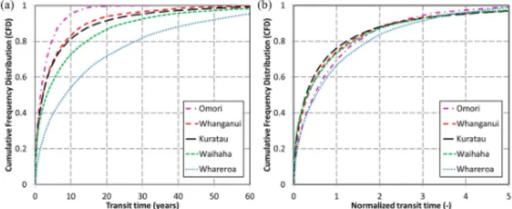
Figure 2.CFDs of transit times for five different watersheds in Lake Taupo region(a)and CFDs with transit times normalized by MTT from Table 1(b).
coincide with surface watersheds shown by solid black lines in Fig. 1b. Therefore, the TTDs in this study are developed from grouped particles based on groundwater water divides in the aquifer.
The particle transit times are used to develop CFD curves for the river network in each of the five selected catchments (Fig. 2a), using the adjustment values estimated earlier to correct for the stream width in MODPATH. The CFDs for each catchment differ in both scale, which is defined by the MTT, and shape, which is defined by the variance, skew-ness, and kurtosis (summarized in Table 1). In order to make a meaningful comparison of shape irrespective of scale, all transit times in a catchment were divided by their respective MTT, hence resulting in a normalized CFD curves for each catchment (see Fig. 2b).
In Fig. 2, the normalized CFD curves for all five catch-ments are roughly similar in shape to the exponentially shaped CFD, which is common for many large water-sheds receiving groundwater recharge over their entire area (Małoszewski and Zuber, 1982; Haitjema, 1995; Abrams, 2012). In the WLTC model settings, the entire modelled area receives groundwater recharge and hence is concep-tually similar to the exponential flow system described by Małoszewski and Zuber (1982). However, it is also noted that the Omori and Whareroa CFDs are virtually identical in shape, while the Kuratau, Waihaha, and Whanganui CFDs tend to have more short and long transit times. This is con-sistent with observations made by Abrams et al. (2013) that watersheds with more partially penetrating streams tend to skew toward shorter and longer transit times with a smaller frequency of intermediate transit times. This implies that the Kuratau, Waihaha, and Whanganui watersheds have a greater incidence of weak sinks; see Gusyev et al. (2013).
3.2 MODPATH tritium concentrations in river water
Table 1.MTT, variance, skewness, and kurtosis for MT3DMS and MODPATH as well as % difference between MT3DMS and MODPATH values of five river catchments.
Parameter CFD WLTC
Omori Whanganui Kuratau Waihaha Whareroa
MTT [yrs]
MODPATH 3.16 6.36 7.51 10.35 16.10
MT3DMS 3.29 6.10 7.05 9.48 15.11
% Difference 4.26 −4.04 −6.16 −8.36 −6.15
Variance [yrs2]
MODPATH 15.97 106.91 176.37 268.98 392.20
MT3DMS 3.94 33.69 39.25 62.62 100.37
% Difference −75.34 −68.49 −77.74 −76.72 −74.41
Skewness [-]
MODPATH 2.49 3.33 3.80 3.10 2.02
MT3DMS 1.19 1.53 1.56 0.94 0.14
% Difference −52.38 −53.93 −59.06 −69.67 −92.97
Kurtosis [-]
MODPATH 9.34 14.85 20.40 13.13 5.65
MT3DMS 2.17 2.04 3.13 0.76 −1.13
% Difference −76.80 −86.24 −84.67 −94.22 −119.97
Figure 3.Annual tritium input and the baseflow tritium concentra-tions calculated by MODPATH for five watersheds from 1955 to 2010. Watersheds are listed in order of increasing MTT.
MODPATH tritium concentrations all have a sharp tritium rise from 1955 to 1970 due to the bomb peak, sharp decline from 1970 to 1990, and approach the natural background tri-tium concentrations from 1990 to 2010 (Fig. 3). Note that in Fig. 3 the watersheds in the legend are not only listed in order of increasing MTT but also in order of highest tritium peak; hence it appears that the smaller the MTT, the higher the tri-tium peak will be. For example, the Omori has the smallest MTT (3.16 yr) in Table 1, and as a result tritium will on aver-age remain in the aquifer for less time than in the other four watersheds. This reduced MTT of groundwater results in less decay of tritium in the subsurface; see Eq. (1). However, it also appears that a narrower range of transit times contributes to the higher peak of the output tritium concentrations in river
water. The Omori has a narrower range of transit times as in-dicated by its small variance (15.97 yr2), meaning that there is a higher frequency of short transit times as compared to the other four catchments. The resulting tritium maximum output for the Omori is greater than at the other watersheds (compare the pink curve in Fig. 3 to the other curves). Sim-ilarly, the Whareroa has the largest MTT (16.1 yr), which is a result of the wide range of transit times reflected in the baseflow, as indicated by its large variance (392.2 yr2). As a result, more tritium is decayed in the subsurface and the pre-bomb tritium input concentrations are also much slower to flush from this catchment. This is manifested as a relatively gradual increase in tritium concentrations in the Whareroa during the bomb tritium peak.
In the 1970s, tritium in rain decreased quickly and fell be-low tritium concentrations in river water (Fig. 3). This rapid decrease in tritium can be observed in the Omori output be-cause of its short MTT with small variance and low removal of tritium due to tritium half-life of 12.32 yr. Conversely, the Whareroa, which has a largest MTT with highest variance, removes much more tritium in the subsurface but concur-rently is slower to flush out the high concentrations of tri-tium. As a result, in the early 1980s, the tritium response for the Omori actually dipped below that of the Whareroa during the model simulation (Fig. 3). As the bomb tritium contin-ued to be removed from the Whareroa, either via discharge or decay, the Omori again returned to the highest tritium con-centration in the early 1990s due to its small MTT and to the shortest transit times (Fig. 3).
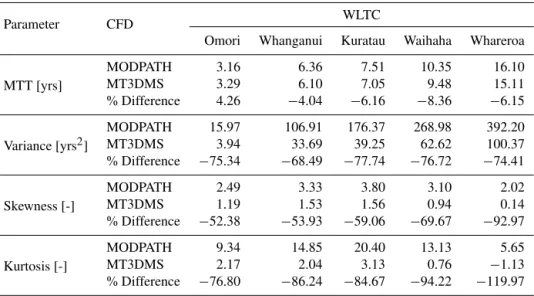
Figure 4.The baseflow tritium concentration calculated by MOD-PATH and MT3DMS (Gusyev et al. 2013) for five watersheds(a–e).
function of the MTT and a constant tritium decay, while true for the peak and present day (at least in this study), was not true in the 1980s. In addition, both MTT and vari-ance were important factors in determining the amplitude of the tritium response curves during the bomb peak in the five river catchments.
3.3 MODPATH and MT3DMS tritium results comparison
MODPATH- and MT3DMS-simulated tritium concentra-tions in TU resulting from the tritium input time series (Fig. 3) are compared in Fig. 4a–e for each of the five catch-ments. The measured tritium concentrations in river water of each catchment are shown by solid circles. For the tritium-calibrated porosity values, the tritium concentrations calcu-lated with MT3DMS by Gusyev et al. (2013) are shown by solid lines, and those calculated with MODPATH are shown by dashed lines in Fig. 4. It is noted that the MODPATH and MT3DMS models yield virtually identical tritium results, with the exception of the peak where there were slight dif-ferences in amplitude in all five river catchments. This sim-ilarity is because the WLTC aquifer system is dominated by advective transport and the tritium decay process (Gusyev et al., 2013), which reduce influence of the dual poros-ity mass transfer coefficient and dispersion–diffusion terms
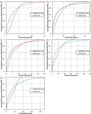
Figure 5. The CFDs of Omori (a), Kuratau (b), Whanganui
(c), Waihaha (d), and Whareroa (e) watersheds calculated by MODPATH and MT3DMS (Gusyev et al., 2013).
in the advection–dispersion equation solved by MT3DMS (Goode, 1996; Zheng and Wang, 1999; Zheng, 2006).
A sensitivity analysis of MODPATH tritium simulations was conducted by varying the porosity by 25 %. Decreas-ing porosity decreases the MTT and, as a result, increases the peak tritium response (MODPATH High in Fig. 4a– e). Increasing porosity increases the MTT and, as a re-sult, decreases the peak tritium response (MODPATH Low in Fig. 4a–e). This is consistent with observations in the previous section where watersheds with higher MTTs had smaller tritium peaks (Fig. 3). In these two porosity cases, the MODPATH CFDs have the same shape but are scaled by percentage values and are not shown in Fig. 2a.
3.4 MODPATH and MT3DMS CFD methodology comparison
points such as constant head, river, drain, and stream cells. All particles discharging to a river cell belonging to a par-ticular watershed were sorted from smallest to largest transit time. Particles released directly on a river cell had a transit time of zero; hence they never entered the aquifer and were removed before constructing the TTD. Finally, because sink cells comprised an artificially large (>8 %) percentage of the watershed surface, the MODPATH transit time correction de-scribed in Abrams (2013) was utilized. To construct the CFD, each particle was weighted based on the recharge assigned to its cell of origin to the total recharge that was assigned to the watershed. Recharge was constant for the entire simu-lation, so the weight assigned to each particle was constant with time. As a result of the above procedure, the transit time for every particle was accounted for; hence this is a TTD that can be applied in Eq. (1).
For the MT3DMS methodology, the CFD for the river net-work is generated by simulating groundwater age concen-trations. An initial concentration of zero age was assigned uniformly at the top of the aquifer and a zero-order decay rate of −1 was assigned to MT3DMS to represent ageing of 1 year per simulation step of 1 year. All dispersion, dif-fusion, and sorption parameters were left unchanged from the tritium simulations. The model was then run for 200 yr to reach steady-state concentrations in river cells. The simu-lated concentration found in each river cell is representative of the groundwater age of all particles mixed together in that cell. This methodology was defined by Cornaton (2004) to simulate a spatial map of groundwaterage, and indeed yields informative cross-sectional images (as shown in Gusyev et al., 2013). To develop the CFD in Fig. 5, the output concen-tration of each river cell was inferred to represent the mean groundwater transit time of all particles reaching that cell (a result of the assigned zero-order degradation rate). The MTT (i.e. output concentration) for each cell was recorded, and these MTTs were sorted from smallest to largest. A weight was assigned to each time based on the ratio of the influx of groundwater to that cell over the total influx of groundwater to the groundwater watershed.
3.5 Comparison of MODPATH and MT3DMS CFD results
In all five cases, the MT3DMS CFDs have less short transit times compared to MODPATH CFDs. Using the MT3DMS PDFs with the convolution integral in Eq. (1) also produces much smaller tritium concentrations for each of the five river catchments, especially around the peak (these results are not shown). While dispersion could potentially result in similar discrepancies, the tritium response curves were insensitive to dispersion values in the WLTC model. Note that MT3DMS CFDs are not required for generating tritium concentrations with MT3DMS. Gusyev et al. (2013) implemented a method to develop MT3DMS CFDs only after the tritium outputs were developed; hence a calibrated value for porosity could
be utilized in developing the MT3DMS CFDs. They were developed to provide a very informative step of how tran-sit times help to shape the tritium output. The shape differ-ences of MT3DMS and MODPATH CFDs are attributed to the limitation of the MT3DMS CFD generation methodol-ogy (Zheng, 2009).
We conducted quantitative comparisons of the five CFDs by calculating higher moments, which required unfolding the data sets by appropriately weighting MODPATH transit times by groundwater recharge and MT3DMS transit times by river discharge. In all cases, the MTT differs by less than 10 % between the MODPATH and MT3D methodologies (see Table 1). This is expected, as both methods take into ac-count the entire range of transit times in the watershed. While the MODPATH method considers each particle explicitly, the MT3DMS method utilizes the average of transit times dis-charging to an individual sink cell. In other words, the very short and very long transit times are only (weakly) included in the distribution developed with MT3DMS via their influ-ence on the mean at individual sink cells. As a result, the variance for all CFDs developed with MT3DMS is less than the variance of the respective MODPATH CFDs (Table 1).
Not only do the MODPATH CFDs explicitly include very short transit times, but these very short transit times also have a higher frequency than any other range of transit times. This is indicated by the progressive decrease in slope of the CFD as transit times increase. In other words, the peak in the fre-quency of transit times occurs with times that are shorter than the mean, resulting in a large positive skew (Table 1). The impact of these more frequent short transit times in the MT3DMS CFDs is (weakly) represented in the average value at each cell. As a result, the MT3DMS CFDs have positive skews as well, but the skews are smaller than those of the re-spective MODPATH CFDs. Similarly, because of the higher frequency of short transit times, the kurtosis is always higher in MODPATH than in MT3DMS.
3.6 Hypothetical examples of MODPATH and MT3DMS CFD methodology
To further illustrate the difference between the two method-ologies, we introduce 1-D, 2-D, and 3-D cases to construct CFDs for the hypothetical river network in idealized aquifers. For clarity, we will henceforth refer to the CFDs generated using the MODPATH methodology as MODPATH CFDs. It is noted that the MT3DMS methodology of generating CFDs can be replicated in MODPATH and that the MOD-PATH methodology of generating MODMOD-PATH CFDs can be replicated in MT3DMS. In all three cases, the MODFLOW model was created to have an MTT of 20.5 yr by assign-ing a constant porosity of 0.3, recharge of 0.445 m year−1 implemented in layer 1, and saturated thickness of 30.48 m. The model was assigned horizontal hydraulic conductivity of 10 m day−1
Figure 6. (a)1-D conceptual model,(b)2-D conceptual model, and
(c)MODPATH and MT3DMS CFDs developed for a 1-D, 2-D, and 3-D conceptual model (dispersion and diffusion transport was dis-abled in the MT3DMS).
model due to the absence of resistance to flow in the ver-tical direction. The model grid was 30 rows by 5 columns with 10 m cell size. The 1-D case conceptualizes a one-dimensional flow aquifer bounded by a no-flow boundary on the left side representing a groundwater divide (black cells) and a constant head boundary of 30.48 m representing the river network on the right side (blue cells). The MODPATH particles were assigned at each cell centre on the top of the aquifer (see plan view in Figure 6a) and produced pathlines to the discharge cells (see the cross-sectional view in Fig. 6a). In the 2-D and 3-D models, the model grid had 1000 rows and 1000 columns with cell size of 10 m, five layers of equal thickness, and a hypothetical river network implemented in layer 1 (Figure 6b). As in the 1-D case, the model was sur-rounded by no-flow cells, and the hypothetical river network was represented by constant head cells of 30.48 m. Both 2-D and 3-D cases are different in vertical hydraulic conductiv-ity setting in the MODFLOW model. For the 2-D model, a vertical hydraulic conductivity of 1000 m day−1
was as-signed to approximate Dupuit–Forchheimer flow. The sim-ulated groundwater contours range from 30.48 m at the head cells to 31.48 m with contour interval of 0.125 m. In the 3-D model, vertical hydraulic conductivity was set equal to the horizontal hydraulic conductivity and resulted in a similar groundwater contour range.
The resulting CFDs of all three cases are demonstrated in Fig. 6c. For the 1-D simulation, the entire range of
tran-sit times (from very short to very long) is represented and the CFD has an exponential shape as expected for the ideal aquifer, which has a MTT of 20.5 yr in our settings; see Hait-jema (1995). For the MT3DMS CFD, however, each of the five discharge cells has the exact same groundwater age con-centration, which is a proxy for MTT of all particles reaching a discharge cell. As a result, the MT3DMS CFD has a pulse shape, shown by the orange curve in Figure 6c, with the jump from 0 to 1 occurring at a transit time of 20.5 yr, which is in-deed the MTT for this aquifer setting. This demonstrates why the MODPATH and MT3DMS methodologies employed for the WLTC model generated very similar MTTs but very dif-ferently shaped CFDs.
In the 2-D case, the MODPATH CFD is exactly the same as the 1-D case, which is expected for this idealized (con-stant recharge, porosity, saturated thickness, and Dupuit– Forchheimer flow) aquifer (Haitjema, 1995) (see Fig. 6c). The 2-D MT3DMS CFD is also similar to its correspond-ing 1-D case but does not have a discrete jump. Rather, there are a few river cells that have a slightly smaller and slightly larger MTT than 20.5 yrs (Fig. 6c). This is likely a result of coarse discretization; a more refined grid would have yielded an even smaller range of MTTs in each cell. Interestingly, the 3-D case with the isotropic aquifer yields a much differ-ent MT3DMS CFD (MTT of 21.86 yr) than the 1-D and 2-D cases (MTT of 20.5 yr) (Fig. 6c). In the 3-D case, resistance to vertical flow is present but minimal since the aquifer is still isotropic. In fact, the impacts of this resistance are not ob-servable for the MODPATH CFD, which is virtually identical to the 1-D and 2-D MODPATH CFDs on the scale of Figure 6c. However, this relatively minor resistance to vertical flow, which was absent in the 1-D and 2-D Dupuit–Forchheimer models, does influence the shape as well as the MTT of the MT3DMS CFD.
To further stress aquifer complexities, we investigated aquifer heterogeneity with the 3-D model. For the aquifer heterogeneity case, we randomly added zones of horizontal hydraulic conductivity with values of 5–30 m day−1
through-out the model domain following analysis introduced by Hait-jema (1995). Though we repeated this with multiple ran-dom hydraulic conductivity zonations, all yielded a sim-ilar response in the MODPATH CFDs of the heteroge-neous aquifer, which was consistent with findings by Hait-jema (1995). However, the heterogeneous MODPATH CFD deviated from the prior MODPATH CFDs, and the MT3DMS CFD deviated further from the homogeneous cases as well (Fig. 6c). The most important observation from this result is that the MT3DMS CFD becomes less shaped like a pulse and more similar to the MODPATH CFD (though for this simple case there is still quite a difference between the MODPATH and MT3DMS CFDs).
local groundwater TTDs that will be represented by varia-tions in MTTs in each of the individual sink cells. For exam-ple, consider a sloping river network where some headwater stream cells will skim water from only the upper portion of the aquifer (physical weak sinks) and hence will have a con-centration (i.e. MTT) in MT3DMS that is younger than the MTT for the entire aquifer (the results of the 3-D simulation are not shown). Other stream cells will take up water that has bypassed those headwater streams and hence will have a concentration (i.e. MTT) in MT3DMS that is older than the MTT for the entire aquifer (Abrams, 2012). These com-plexities will cause the MT3DMS CFD simulation to further deviate from the pulse shape for the 1-D case shown in Fig. 6 and, in theory, possibly approach the MODPATH CFD sim-ulation. Indeed, this is why the MT3DMS CFDs shown in Fig. 5 are not pulse-shaped, but rather have approached the shape of the MODPATH CFD for each of the five WLTC wa-tersheds due to complexities of the WLTC model settings.
4 Concluding remarks
In this work, we presented an approach to calibrate the steady-state MODFLOW-MODPATH model to measured tri-tium concentrations in river water at baseflows of the five river catchments of the WLTC. In the previous study, Gusyev et al. (2013) developed the steady-state groundwater flow MODFLOW model for the WLTC and calibrated the tran-sient MT3DMS model to tritium measurements in river wa-ter. The model had several important features: the uniform 80 m model grid to include small surface water features, 10 zones of groundwater recharge, and 5 zones of aquifer poros-ity. The results of the groundwater flow model indicated vari-able saturated thickness and groundwater elevations ranging from 357 m above mean sea level at the Lake Taupo shore to over 1000 m in the northern part of the model domain. In this study, the calibrated MODFLOW-MT3DMS model was used with particle-tracking MODPATH to produce TTDs and a map of transit times for the WLTC river network. The MOD-PATH TTDs were convolved to obtain tritium concentration in river water for the five river catchments of the WLTC. The tritium concentrations obtained with MODPATH show a good match to measured tritium time series despite account-ing only for advective transport.
When generating tritium concentrations with MODPATH TTDs, it is important to understand many implicit assump-tions of the convolution integral. First, there is no spatial component in the convolution integral; time is the only vari-able. As a result, input tritium concentrations at each time t are assumed to be spatially uniform over each individual watershed. This is a valid assumption for tritium in precip-itation, but it may not be true for other chemicals such as nitrate. Second, λis assumed to be constant over time and the entire aquifer thickness. Again, this assumption is valid for a non-reactive tritium tracer, but may not be for
describ-ing zonal reaction processes such as denitrification, which is dependent on dissolved oxygen and organic matter concen-trations in the aquifer. Third, the TTDs are based on steady-state model runs with temporally constant recharge and sat-urated thicknesses. The MODPATH model has the capabil-ity of conducting transient simulations, and transient TTDs can be constructed by weighting each particle based on the recharge when it entered the aquifer. However, obtaining tri-tium concentrations from transient TTDs is non-trivial. A new CFD is required for each year that TU is calculated in the transient simulation – in other words, if calculating TU at yearly intervals for 200 years to construct a TU curve would require 200 CFDs. Finally, any travel times and re-sulting reactions in the unsaturated zone and river beds are not considered. For this particular watershed, these assump-tions are reasonable; this is especially true since the tracer is tritium. The assumptions underlying the convolution integral may lead to conceptual errors when studying other dissolved constituents in groundwater such as nitrates.
Consequently the MODPATH and MT3DMS CFDs were compared to understand better the model results and assump-tions for generating CFDs in river networks. Even though the MT3DMS CFDs for the river network are only yielding approximations of the true transit time CFD, the informa-tion they provide is still useful. Most importantly, they still yield the correct MTT for the watershed. Furthermore, the MT3DMS distribution provides insight into the variations from an idealized watershed described in Haitjema (1995) and Abrams (2012). These factors include weak sinks, vari-ations in saturated thickness, varivari-ations in recharge, etc. The MODPATH and MT3DMS CFDs must be interpreted differ-ently, with the understanding that only MODPATH is pro-viding the TTD that should be used in the convolution in-tegral. This may be seen by the match of MODPATH tri-tium responses using the CFD in conjunction with the con-volution integral to the MT3DMS tritium outputs (Fig. 5). Using the MT3DMS CFDs with the convolution integral yields a much different (and inaccurate) tritium response because, even though they have a similar MTT, the shape of the MT3DMS CFDs generally has both more short and long transit times than MODPATH. Hence, we promote both CFDs when using MODPATH and/or MT3DMS, as the tran-sit time CFD generated by MODPATH is necessary to gener-ate tritium and nitrgener-ate output functions with Eq. (1), but the MT3DMS CFD allows us to understand the variation from idealized conditions. This would be particularly useful in as-sessing when a lumped parameter model could have been used in place of a distributed parameter model, which would be valuable information for future studies.
unresponsiveness to air exchange processes in river water. In precipitation, tritium concentrations are independent of air temperature and pressure, and measured monthly at many ground stations of the Global Network of Isotopes in Pre-cipitation established by the International Atomic Energy Agency (IAEA/WMO, 2014). For the subsurface processes, tritium, being a part of the water molecule, does not re-act with aquifer matrix or dissolved chemicals in ground-water. In river water, the tritium concentrations discharged with groundwater remain almost unaffected by evaporation and exchange with air. Because of its radioactive decay, tritium concentrations in groundwater are still dependent on the travel times despite constant tritium inputs over re-cent decades in the Southern Hemisphere and can be deter-mined with high detection accuracy (Morgenstern and Tay-lor, 2009). From now on, the tritium time series measure-ments in river water of the Northern Hemisphere will be valu-able for model calibration, especially after tritium concentra-tions in precipitation return to pre-bomb levels in the next decades (Stewart et al., 2012).
Acknowledgements. We thank two Anonymous Referees and the Editor for their insightful comments that allowed us to highlight the novelty of our work and to improve the presentation of our findings. We also thank J. Hadfield of the Waikato Regional Council, New Zealand, for his support that initiated this study.
Edited by: M. Bakker
References
Abrams, D. B.: Generating nitrate response functions for large re-gional watersheds, PhD Thesis, Indiana University, Blooming-ton, 85 p., 2012.
Abrams, D.: Correcting transit time distributions in coarse MODFLOW-MODPATH models, Groundwater, 51, 474–478, doi:10.1111/j.1745-6584.2012.00985.x, 2013.
Abrams, D., Haitjema, H., and Kauffman, L.: On modeling weak sinks in MODPATH, Ground Water, 51, 597–602, doi:10.1111/j.1745-6584.2012.00995.x, 2013.
Boronina, A., Renard, P., Balderer, W., and Stichler, W.: Ap-plication of tritium in precipitation and in groundwater of the Kouris catchment (Cyprus) for description of the re-gional groundwater flow, Appl. Geochem., 20, 1292–1308, doi:10.1016/j.apgeochem.2005.03.007, 2005.
Cornaton, M. F.: Deterministic models of groundwater age, life ex-pectancy and transit time distributions in advective-dispersive systems, PhD Thesis, University of Neuchâtel, Switzerland, 165 p., 2004.
Eberts, S. M., Bohkle, J. K., Kauffman, L. J., and Jurgens, B. C.: Comparison of particle-tracking and lumped-parameter age-distribution models for evaluating vulnerability of pro-duction wells to contamination, Hydrogeol. J., 20, 263–282, doi:10.1007/s10040-011-0810-6, 2012.
Fienen, M., Hunt, R. J., Krabbenhoft, D. P., and Clemo, T.: Ob-taining parsimonious hydraulic conductivity fields using head and transport observations: A Bayesian geostatistical param-eter estimation approach, Water Resour. Res., 45, W08405, doi:10.1029/2008WR007431, 2009.
Goode, D. J.: Direct simulation of groundwater age, Water Resour. Res., 32, 289–296, 1996.
Gusyev, M. A., Toews, M., Morgenstern, U., Stewart, M., White, P., Daughney, C., and Hadfield, J.: Calibration of a transient trans-port model to tritium data in streams and simulation of ground-water ages in the western Lake Taupo catchment, New Zealand, Hydrol. Earth Syst. Sci., 17, 1217–1227, doi:10.5194/hess-17-1217-2013, 2013.
Haitjema, H. M.: On the residence time distributions in groundwa-tersheds, J. Hydrol., 172, 127–146, 1995.
Harbaugh, A. W., Banta, E. R., Hill, M. C., and McDonald, M. G.: MODFLOW-2000, the U.S. Geological Survey modular ground-water model – User guide to modularization concepts and the Ground-Water Flow Process, Open-File Report 00-92, US Geo-logical Survey, 2000.
Hunt, R. J., Feinstein, D. T., Pint, C. D., and Anderson, M. P.: The importance of diverse data types to calibrate a watershed model of the Trout Lake Basin, Northern Wisconsin, USA, J. Hydrol., 321, 286–296, doi:10.1016/j.jhydrol.2005.08.005, 2005. IAEA/WMO: Global Network of Isotopes in Precipitation, The
GNIP Database, available at: http://www.iaea.org/water (last ac-cess: June 2014), 2014.
Jurgens, B. C., Böhlke, J. K., and Eberts, S. M.: TracerLPM (Ver-sion 1): An Excel®workbook for interpreting groundwater age distributions from environmental tracer data: U.S. Geological Survey Techniques and Methods Report 4-F3, 60 p., 2012. Kauffman, L. J., Baehr, A. L., Ayers, M. A., and Stackelberg, P. E.:
Effects of land use and travel time on the distribution of nitrate in the Kirkwood-Cohansey aquifer system in southern New Jer-sey, US Geological Survey Water-Resources Investigations Re-port 01-4117, 49 p., 2001.
Małoszewski, P. and Zuber, A.: Determining the turnover time of groundwater systems with the aid of environmental trac-ers 1. Models and their applicability, J. Hydrol., 57, 207–231, doi:10.1016/0022-1694(82)90147-0, 1982.
McDonnell, J. J., McGuire, K., Aggarwal, P., Beven, K., Biondi, D., Destouni, G., Dunn, S., James, A., Kirchner, J., Kraft, P., Lyon, S., Małoszewski, P., Newman, B., Pfister, L., Rinaldo, A., Rodhe, A., Sayama, T., Seibert, J., Solomon, K., Soulsby, C., Stewart, M., Tetzlaff, D., Tobin, C., Troch, P., Weiler, M., Western, A., Wörman, A., and Wrede, S.: How old is streamwa-ter? Open questions in catchment transit time conceptualiza-tion, modelling and analysis, Hydrol. Process., 24, 1745–1754, doi:10.1002/hyp.7796, 2010.
McGuire, K. J. and McDonnell, J. J.: A review and evaluation of catchment transit time modelling, J. Hydrol., 330, 543–563, doi:10.1016/j.jhydrol.2006.04.020, 2006.
Morgenstern, U.: Lake Taupo streams – Water age distribution, frac-tion of landuse impacted water, and future nitrogen load. En-vironment Waikato Technical Report TR 2007/26, Document #1194728, 28 p., 2007.
Morgenstern, U. and Taylor, C. B.: Ultra Low-level tritium measure-ment using electrolytic enrichmeasure-ment and LSC, Isotop. Environ. Health Stud., 45, 96–117, doi:10.1080/10256010902931194, 2009.
Pint, C. D., Hunt, R. J., and Anderson, M. P.: Flowpath delineation and ground water age, Allequash Basin, Wisconsin, Ground-water, 41, 895–902, doi:10.1111/j.1745-6584.2003.tb02432.x, 2003.
Pollock, D. W.: User’s Guide for MODPATH/MODPATH-PLOT, Version 3: A particle tracking post-processing package for MOD-FLOW, the U.S. Geological Survey finite-difference ground-water flow model, US Geological Survey Open-File Report 94-464, 249 p., 1994.
Sanford, W.: Calibration of models using groundwater age, Hydro-geol. J., 19, 13–16, doi:10.1007/s10040-010-0637-6, 2010. Schlumberger Water Services (SWS): Visual MODFLOW User’s
Manual, Version 2010.1, 676 p., 2010.
Starn, J. J., Bagtzoglou, A. C., and Robbins, G. A.: Us-ing atmospheric tracers to reduce uncertainty in groundwater recharge areas, Groundwater, 48, 858–868, doi:10.1111/j.1745-6584.2010.00674.x, 2010.
Stewart, M. K., Morgenstern, U., McDonnell, J. J., and Pfis-ter, L.: The “hidden streamflow” challenge in catchment hy-drology: a call to action for stream water transit time anal-ysis, invited Commentary, Hydrol. Process., 26, 2061–2066, doi:10.1002/hyp.9262, 2012.
Stichler, W., Małoszewski, P., Bertleff, B., and Watzel, R.: Use of environmental isotopes to define the capture zone of a drinking water supply situated near a dredge lake, J. Hydrol., 362, 220– 223, doi:10.1016/j.jhydrol.2008.08.024, 2008.
Szabo, Z., Rice, D. E., Plummer, L. N., Busenberg, E., Drenkard, S., and Schlosser, P.: Age dating of shallow groundwater with chlo-rofluorocarbons, tritium/helium 3, and flow path analysis, south-ern New Jersey coastal plain, Water Resour. Res., 32, 1023–1038, doi:10.1029/96WR00068, 1996.
Troldborg, L., Refsgaard, J. C., Jensen, K. H., and Engesgaard, P.: The Importance of Alternative Conceptual Models for Simula-tion of ConcentraSimula-tions in a Multi-aquifer System, Hydrogeol. J., 15, 843–860, 2007.
US EPA: Handbook of Ground Water and Wellhead Protec-tion, US Environmental Protection Agency (US EPA), Report EPA/625/R-94001, 288 p., 1994.
Vant, B. and Smith, P.: Nutrient concentrations and groundwa-ter ages in 11 streams flowing into Lake Taupo, Environment Waikato Technical Report 2002/18R, Doc #767068, 18 p., 2002. Walker, J. F., Saad, D. A., and Hunt, R. J.: Dynamics of CFCs in northern temperate lakes and adjacent groundwater, Water Re-sour. Res., 43, W04423, doi:10.1029/2005WR004647, 2007. Weissman, G. S., Zhang, Y., LaBolle, E. M., and Fogg, G. E.:
Dis-persion of groundwater age in an alluvial aquifer system, Wa-ter Resour. Res., 38, 16-1–16-13, doi:10.1029/2001WR000907, 2002.
Zheng, C.: MT3DMS v. 5.2 Supplementary User’s Guide, Technical Report, University of Alabama, 41 p., 2006.
Zheng, C.: Recent developments and future directions for MT3DMS and related transport codes, Groundwater, 47, 620– 625, doi:10.1111/j.1745-6584.2009.00602.x, 2009.