Landcover and crop type classification with intra-annual times series of sentinel-2 and machine learning at central Portugal

i

Itzá Alejandra Hernández Sequeira

LANDCOVER AND CROP TYPE CLASSIFICATION

with intra-annual times series of sentinel-2 and

machine learning at Central Portugal

ii

LANDCOVER AND CROP TYPE CLASSIFICATION

with intra-annual times series of sentinel-2 and machine learning at Central Portugal

Dissertation supervised by:

Ph.D. Mário Sílvio Rochinha de Andrade Caetano

Associate Professor, Nova Information Management School (NOVA IMS) University of Nova, Lisbon, Portugal

Ph.D. Filiberto Pla Bañón

Professor, Institute of New Imaging Technologies (INIT) University of Jaume I (UJI)

Castellón, Spain

Ph.D. Hugo Alexandre Gomes da Costa

Invited Lecturer, Nova Information Management School (NOVA IMS) University of Nova, Lisbon, Portugal

iii

DECLARATION OF ORIGINALITY

I declare that the work described in this document is my own and not from someone else. All the assistance I have received from other people is duly acknowledged and all the sources (published or not published) are referenced.

This work has not been previously evaluated or submitted to NOVA Information Management School or elsewhere.

Lisboa, February 24, 2020

Itzá Alejandra Hernández Sequeira

iv

ACKNOWLEDGMENTS

First, I would like to thank my supervisor Mário Caetano for allowing Geotech master students to develop research in the Direção-Geral do Território (DGT); for visualizing the project and encouraging me to take this challenge. Additionally, I would like to thank my co-supervisor Hugo Costa and (my un-official co-supervisor) Pedro Benevides from the Divisão de Informação Geográfica (DIG) for their helpful guidance and all the constant feedback provided to this work; and to my co-supervisor Filiberto Plá for his enthusiasm on the thesis topic and constructive suggestions provided. Special thanks to William Martínez, because his applied coding knowledge to geospatial information was essential to develop many of the scripts. I learned a lot from their insights in the remote sensing and land cover mapping field; working alongside them was a great professional experience.

Also, I express my gratitude towards the Erasmus Mundus Program for financing students from all over the world to pursue their academic development with the Master in Geospatial Technologies. The multi-cultural environment we are surrounded by makes us more tolerant and open towards others. Many thanks to Marco Painho, Christoph Brox, and Joaquín Huerta for coordinating this program through the three universities. Special thanks to Joel Silva from NOVA IMS for the codes he provided during the remote sensing course as they were a fundamental input to this work.

Additionally, I am grateful for my GeoTech family, which is an enthusiastic and talented group of people. I was encouraged by the quality of their work in every project they delivered. Especially during the Geomundus Conference that we organized, that is an excellent memory of outstanding teamwork. Special thanks to the wonderful people that supported me until the very end of the master Carlos, Francisco, Mihail, and Vicente; it was a pleasure sharing many Lisbon memories with you.

Finally, I cannot thank enough my family in Nicaragua; they are the real strength behind every project I achieve.

This thesis was developed under the framework of the project foRESTER (PCIF/SSI/0102/2017) funded by Fundação para a Ciência e Tecnologia

v

LANDCOVER AND CROP TYPE CLASSIFICATION

Portugal

ABSTRACT

Land cover and crop type mapping have benefited from a daily revisiting period of sensors such as MODIS, SPOT-VGT, NOAA-AVHRR that contains long time-series archive. However, they have low accuracy in an Area of Interest (ROI) due to their coarse spatial resolution (i.e., pixel size > 250m). The Copernicus Sentinel-2 mission from the European Spatial Agency (ESA) provides free data access for Sentinel 2-A(S2a) and B (S2b). This satellite constellation guarantees a high temporal (5-day revisit cycle) and high spatial resolution (10m), allowing frequent updates on land cover products through supervised classification. Nevertheless, this requires training samples that are traditionally collected manually via fieldwork or image interpretation. This thesis aims to implement an automatic workflow to classify land cover and crop types at 10m resolution in central Portugal using existing databases, intra-annual time series of S2a and S2b, and Random Forest, a supervised machine learning algorithm. The agricultural classes such as temporary and permanent crops as well as agricultural grasslands were extracted from the Portuguese Land Parcel Identification System (LPIS) of the Instituto de Financiamento da Agricultura e Pescas (IFAP); land cover classes like urban, forest and water were trained from the Carta de Ocupação do Solo (COS) that is the national Land Use and Land Cover (LULC) map of Portugal; and lastly, the burned areas are identified from the corresponding national map of the Instituto da Conservação da Natureza e das Florestas (ICNF). Also, a set of preprocessing steps were defined based on the implementation of ancillary data allowing to avoid the inclusion of mislabeled pixels to the classifier. Mislabeling of pixels can occur due to errors in digitalization, generalization, and differences in the Minimum Mapping Unit (MMU) between datasets. An inner buffer was applied to all datasets to reduce border overlap among classes; the mask from the ICNF was applied to remove burned areas, and NDVI rule based on Landsat 8 allowed to erase recent clear-cuts in the forest. Also, the Copernicus High-Resolution Layers (HRL) datasets from 2015 (latest available), namely Dominant Leaf Type (DLT) and Tree Cover Density (TCD) are used to distinguish

vi

between forest with more than 60% coverage (coniferous and broadleaf) such as Holm Oak and Stone Pine and between 10 and 60% (coniferous) for instance Open Maritime Pine. Next, temporal gap-filled monthly composites were created for the agricultural period in Portugal, ranging from October 2017 till September 2018. The composites provided data free of missing values in opposition to single date acquisition images. Finally, a pixel-based approach classification was carried out in the “Tejo and Sado” region of Portugal using Random Forest (RF). The resulting map achieves a 76% overall accuracy for 31 classes (17 land cover and 14 crop types). The RF algorithm captured the most relevant features for the classification from the cloud-free composites, mainly during the spring and summer and in the bands on the Red Edge, NIR and SWIR. Overall, the classification was more successful on the irrigated temporary crops whereas the grasslands presented the most complexity to classify as they were confused with other rainfed crops and burned areas.

vii

KEYWORDS

Land Cover Mapping Crop type Mapping Random Forest

Automatic Sample Extraction Intra-annual time series Portugal

viii

ACRONYMS

CAP – Common Agricultural Policy

COS – Carta de Uso e Ocupação do Solo (Portuguese of LCLU)

DGT – Direção-Geral do Território - General Directorate for Territorial Management FCT - Fundação para a Ciência e Tecnologia - Foundation for Science and Technology. foRESTER – Rede de sensores combinada com modelação da propagação do fogo integrado num sistema de apoio à decisão para o combate a incêndios florestais - Data fusion of sensor networks and fire spread modelling for decision support in forest fire suppression.

EU – European Union

HRL – High-Resolution Layers

ICNF - Instituto da Conservação da Natureza e das Florestas - Institute for Nature Conservation and Forests

IFAP – Instituto de Financiamento da Agricultura e Pescas - Agriculture and Fisheries Financing Institute

INSPIRE– Infrastructure for spatial information in Europe IPSTERS - IPSentinel Terrestrial Enhanced Recognition System LCLU – Land Cover Land Use

LPIS - Land Parcel Identification System NCPA – National Control and Paying Agency OTS – On-The-Spot

ix

INDEX OF THE TEXT

ACKNOWLEDGMENTS ... iv ABSTRACT ... v KEYWORDS ... vii ACRONYMS ... viii INDEX OF TABLES ... x INDEX OF FIGURES ... xi 1 INTRODUCTION ... 1 1.1 Background ... 1

1.2 Problem Statement and Motivation ... 1

1.3 Research Question ... 4

1.4 Aim ... 4

1.5 Objectives ... 5

1.6 Thesis structure ... 5

2 LITERATURE REVIEW ... 6

2.1 Land cover mapping ... 6

2.2 Crop type mapping ... 7

2.3 Sentinel-2 time series ... 8

2.3.1 Time series imagery ... 8

2.3.2 Intra-annual and Inter-annual ... 8

2.3.3 Gap-filled image composites ... 8

2.4 Machine Learning – Statistical Learning ... 9

2.4.1 Machine Learning Process ... 9

2.4.2 Supervised and Unsupervised Learning ... 11

2.4.3 Regression, Classification, and Clustering ... 11

2.4.4 Random Forest (RF) ... 11

3 METHODOLOGY ... 14

3.1 Study area ... 14

3.2 Data ... 15

3.2.1 Ancillary data ... 16

3.2.2 Remote Sensing Data ... 21

3.3 Methods ... 23

3.3.1 Software and device specifications ... 25

3.3.2 Preprocessing of the reference datasets ... 25

3.3.3 Preprocessing of the intra-annual time series of Sentinel 2 ... 31

x

3.3.5 Accuracy Assessment of the model performance and map production ... 41

4 RESULTS AND DISCUSSION ... 44

4.1 Variable importance ... 44

4.2 Land Cover and Crop Type Classification ... 45

4.2.1 Quantitative Map Evaluation ... 46

4.2.2 The relevance of time series in crop phenology ... 50

4.2.3 Visual inspection ... 51

5 CONCLUSIONS ... 56

5.1 Limitations and Recommendations ... 57

6 BIBLIOGRAPHIC REFERENCES ... 59

7 ANNEXES ... 66

7.1 External scripts ... 66

7.2 Land Cover and Crop Type nomenclature ... 66

7.3 RGB color ramp for the Land Cover and Crop Type Classes ... 69

7.4 Crop Calendar ... 71

7.5 Confusion matrix ... 72

INDEX OF TABLES

Table 2 Nomenclature for Land Cover and Crop type ... 20

Table 3 Specifications of the Sentinel-2 bands ... 21

Table 4 Rules for the crossing of COS polygons with HRL ... 30

Table 5 Spectral indices derived from the monthly composites ... 32

Table 6 Training and testing samples for the area ... 34

Table 7 Training and testing samples for the four classes with imbalance ... 35

Table 8 User-defined parameters for Grid Search ... 40

Table 9 Ranking of the hyperparameters grid using 10-fold cross-validation ... 40

Table 10 Cross-validation results for the best model (10 folds, mean and standard deviation) ... 41

Table 11 Binary confusion matrix ... 42

Table 12 Extraction of the 10 most important feature in the classification and the 10 least relevant for the selected model ... 45

Table 13 Land Cover and Crop Type results of the classification. The Overall Accuracy (OA%), User's Accuracy (UA%), Producer's Accuracy (PA%), F1-SCORE (F1%), and the number of testing samples (N°) are reported for the RF model with 500 trees. . 48

xi

Table 14 Confusion matrix for the Land Cover and Crop Type classification at LV4 ... 49

INDEX OF FIGURES

Figure 2 Stratification of Continental Portugal [40]. Scale 1:3,000,000. ... 14

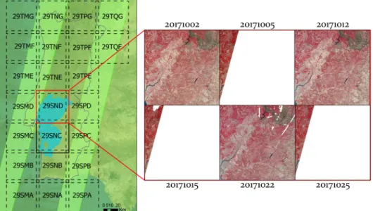
Figure 3 Sentinel-2 orbit, swath, and tilling for the study area and images acquired for October 2017 in the tile 29SND. ... 22

Figure 4 Flowchart for the automatic production of a land cover and crop type map in central Portugal ... 24

Figure 5 Data preprocessing workflow for reference datasets ... 26

Figure 6 Area covered by the 10 most abundant crops in hectares ... 26

Figure 7 Distribution of the tree main crop parcels by area (ha) ... 27

Figure 8 IFAP parcels pre-processing: inverse buffer (- 40m) ... 27

Figure 9 COS2018 polygon overlaid with the burned mask, Maritime Pine OBJECTID: 493848 and Eucalyptus OBJECTID: 415864. Scale 1:7,000 (1) and 1:25,000 (2). ... 29

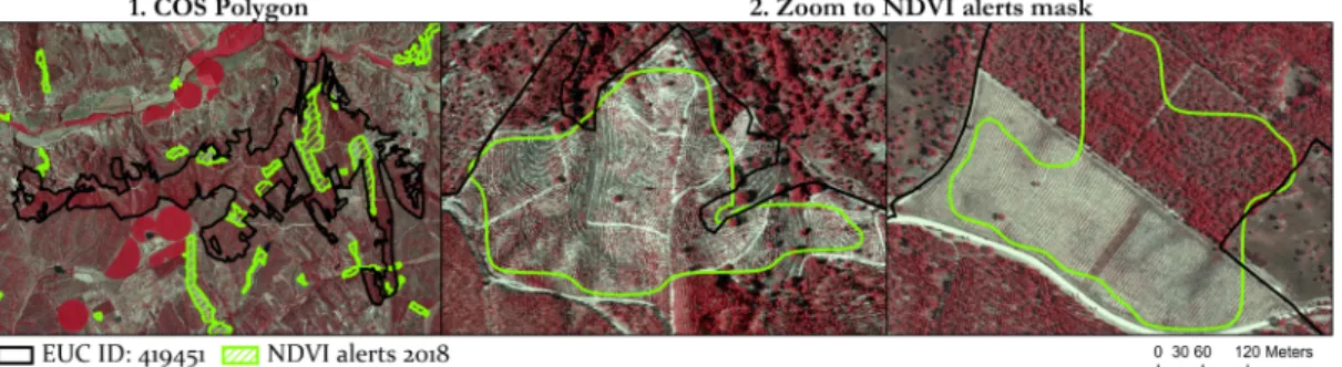
Figure 10 NDVI alerts in a Eucalyptus plantation (COS 2018 OBJECTID: 382944). Scale 1:80,000 (1) and 1:6,000 (2). ... 29

Figure 11 DLT (1) and TCD (2) rule for shrublands (COS OBJECTID: 592293). Scale 1:20,000. ... 30

Figure 12 Preprocessing workflow for Sentinel-2 intra-annual time series ... 31

Figure 13 Image acquisition with less than 50% cloud cover for tile 29SND in July 2018 ... 32

Figure 14 Series of monthly cloud-free reflectance composites at 10m resolution (October 2017 to September 2018) the pointed area corresponds to an agricultural area. ... 33

Figure 15 Supervised learning workflow ... 34

Figure 16 Automatic sample extraction for IFAP 2018 (Maize OSAID: 4358737-training; 36821510-testing). Scale 1:12,500. ... 35

Figure 17 Automatic sample extraction for COS 2018 (Cork Oak OBJECTID: 382944). Scale 1:20,000 (1) and 1:5,000 (2) and (3). ... 36

Figure 18 Training and testing samples for the biogeographical region divided between tiles 29SND and 29SNC. ... 36

Figure 19 Extraction of the spectral features for training and testing datasets ... 37

Figure 20 Dataframe of the training dataset containing the 115,880 samples with 180 extracted features ... 38

xii

Figure 21 Correlation between spectral signatures for bands and indices for October 2017 ... 39 Figure 22 Accuracy assessment and map production workflow ... 41 Figure 23 (a) Land Cover and Crop Type in raster format, (b) detail of the map, (c)

false-color (RGB: b8, b4, and b3) for august 2018 Sentinel-2a composite, (d) the Iberian Peninsula with Portugal and Stata 214 highlighted. ... 46 Figure 24 Average surface reflectance in the Red Edge (band 5), NIR (band 8a), and SWIR (b11) for wheat (a), rice (b), and vineyards (c) from October17 to September18. ... 51 Figure 25 COS 2018 (OBJECTID: 491011) polygon pre and post-processed comparison to predictions for the class Open Maritime Pine Forest. Scale: 1:30.000 ... 52 Figure 26 COS 2018 (OBJECTID: 382944) polygon pre and post-processed comparison to predictions for the class Holm Oak. Scale: 1:10.000 ... 53 Figure 27 IFAP 2018 (OSAID: 4410598) polygon pre and post-processed comparison to predictions for the class Orchards. Scale: 1:6000 ... 54 Figure 28 (a) Land Cover and Crop Type in raster format with three locations on the border of the Sentinel-2 tiles 29SND (upper) and 29SNC (lower), (b) Tejo estuary (c) border of Santarém and Sétubal, (d) location near Évora. ... 55

1

1 INTRODUCTION

1.1 Background

There is a need to quantify land cover and its changes over time in a precise and timely way for monitoring human and physical environments [1] as well as for providing information to support studies, research, and sustainable development policies [2]. The constant changes in land cover dynamics and the seasonality of crops demand a spatial and temporal continuity in the mapping of the areas of interest. Nowadays, it is possible to produce robust large-scale land cover mapping automatically using supervised classification, time series of high-resolution optical imagery, and existing databases for data training and validation [3]. The new paradigm in land cover production -Land Cover 2.0- takes advantage on the developments in computer hardware and software; increased spatial, spectral, and temporal resolutions of satellite imagery; open-access data and automated data processing using classification algorithms to generate timely, reproducible and accurate land cover maps [4]. Currently, it is possible to classify large geographic areas over multiple decades at an annual time step, as reported by Hermosilla et al. (2018) [5] that generated a 29-year data cube of land cover for the years 1984 to 2012. Moreover, automated systems as the Sen2-Agri can ingest and process multi-sensor imagery (Sentinel-2 and Landsat 8 time series) for operational agriculture monitoring systems [6].

1.2 Problem Statement and Motivation

The General Directorate for Territorial Management (DGT) in Portugal is the entity responsible for producing two land-use maps for mainland Portugal: the CORINE Land Cover (CLC) and the Carta de Uso e Ocupação do Solo (COS) that is the official Land Cover Land Use (LCLU) of the country. From one side, the CLC is a European project with a minimum mapping unit of 25 ha and 44 thematic classes with five years of reference (1990, 2000, 2006, 2012 and 2018) while the COS is a national product with a minimum mapping unit of 1 ha, 88 classes in 2018 and 6 years of reference (1990, 1995, 2007, 2010, 2015 and 2018) [7]. Mapping 88 classes at a spatial resolution of 1 ha require very high-resolution orthophoto maps and rely mainly on visual interpretation for its competition. Despite the significant improvement in the reduction of production time from 10 years in 2000 to 3 years in 2018, COS remains a product that takes time and human effort.

2

During the year 2017, Portugal registered an extreme wildfire season with a record of 500,000 ha burned and more than 100 human lives lost. These natural hazards, along with droughts and heatwaves, are intensifying in the Mediterranean basin due to climate change [8]. Wildfires represent a severe hazard that can have negative impacts on society and the environment; they can become a disaster when a significant number of people in vulnerability are exposed, consequentially human lives are lost and livelihoods damaged [9]. Characterizing and predicting fire spread and behavior is applied to determine higher risk areas and firefighting strategies to minimize damage [10]. In order to predict fire-spread and behavior, fire simulation models use gridded geospatial information as input data for fire simulation. This data can comprise elements such as topography (i.e., elevation, aspect, and slope), weather conditions, and fuel types (i.e., surface fuel type and canopy metrics) [11].

As part of a decision support system for firefighting, DGT aims to provide an annual Land Cover (LC) map for fire propagation models in 2020 with fewer thematic classes than the COS for central Portugal. This map is intended to be prepared before the fire season and will enable the updated characterization of the terrain, as well as areas that burned and vegetation cuts. It will be produced in raster format (10m pixel size) and based on supervised classification over the satellite time series of Sentinel-2. The realization of this annual LC map is part of three projects: the “IPSentinel Terrestrial Enhanced Recognition System” (IPSTERS) whose primary goal is the implementation of AI algorithms in the digestion of Big Data for remote sensing in order to derive LCLU maps [12]; the “Data fusion of sensor networks and fire spread modeling for decision support in forest fire suppression” (foRESTER) that intends to derive LC maps from satellite imagery and ground data for near-real-time (NRT) fire spread predictions (FSP) [13]; and the Sustainable landSCAPE planning model for rural FIREs prevention (SCAPE FIRE). Nonetheless, the production of these LC maps is dependent on the availability of sample data, and typically, training samples are acquired manually through visual interpretation or fieldwork. The challenge remains to train supervised algorithms without human intervention in sample labeling. Instead, to acquire training samples from pre-existing datasets filtered with auxiliary information to discard possible data mislabeling.

The automatic sample extraction from existing datasets for supervised classification is ongoing research at DGT, using Central Portugal as a study case. Lüdtke, D. (2018) [14] implemented the EUROSTAT’s Land Use/Cover Area Statistical Survey (LUCAS) database as training data and Sentinel-2 time series for monthly and annual

3

classification. She concluded that the leading cause of the low Overall Accuracy (OA) achieved (58% for six classes) was the uncertainties of the LUCAS database. Yet, a compelling finding was that the simultaneous use of the bands for the period of analysis (November 2016 to October 2017) resulted in higher accuracy than using monthly data. Later, Blanco, W. (2019) [15] used training data from an old map of COS 2015 to classify imagery of 2017 and using Sentinel-2 seasonal composites following a Best Available Pixel (BAP). The overall accuracy achieved using 13 features resulted in and 73% for six 61% in nine classes for the baseline. He concluded that although COS is a valuable source for sample extraction, it was not possible to increase the OA after refinements on the training data. Still, the BAP composites provided a free-cloud efficient input for a seasonal LC mapping. At present, DGT is implementing some other approaches to extract consistently labeled training samples from outdated maps; a novel-approach tested is the implementation of unsupervised clustering methods based on the methodology of Paris, C. (2019) [16]. In addition, training samples have been obtained from the visual interpretation of orthophoto maps and on auxiliary data [17]. This approach was carried out for Continental Portugal includes using Landsat Time-Series to derive LCLU maps from 2010 to 2015 achieving accuracies of 87.5% for the 2010 map using 15 classes.

This thesis was developed under the framework of the project foRESTER, and it investigates the possible results of implementing current research at DGT for automatically deriving samples from ancillary data for supervised classification. The methodology corresponds to the protocol for Land Cover and Crop Mapping 2018 for Tejo and Sado.

4 1.3 Research Question

When performing supervised image classification, several algorithms can be applied, and different data sources can be utilized for training the classifier. Depending on the number of target classes, the overall accuracy of the map fluctuates. The more classes are added to the classification, the higher the probability of misclassifications and, therefore, the reduction in the ability of the classifier to map the classes accurately. To create an automatic map, the main task is to generate a stable workflow for classifying satellite imagery in a reproducible way. Developing the present research at DGT and the availability of time series of Sentinel-2 and the up to date ancillary datasets (COS 2018, IFAP parcels 2018 and ICNF burned areas 2018), three research questions are proposed:

1. How accurate is it to classify 31 classes of land cover and crop types at 10m resolution?

2. Which are the most important features/variables to consider when using intra-annual time series?

3. When performing automatic sample extraction, can a set of pre-processing rules allow us to extract spectral signatures of the classes suitable for image classification?

1.4 Aim

This investigation project aims to generate an automatic land cover and crop type map in raster format using in situ and up-to-date data, satellite imagery, and machine learning algorithms. The automatization method relies on the retrieval of the spectral signatures of the land cover and crop types from intra-annual time-series imagery of Sentinel-2 at the pixel level taking advantage of the availability from COS 2018 land cover dataset, and IFAP 2018 monitored agricultural parcels as well as ICNF 2018 burned areas. These areas will serve as training and testing input to the Random Forest classifier, allowing to implement the supervised machine learning method for land cover and crop type classification.

5 1.5 Objectives

• Contribute to an automatic supervised classification workflow to produce land-cover and crop type maps.

• _{Review the existing state-of-the-art in machine learning and multi-temporal optical} imagery for classifying land cover and crop type areas.

• Classify land cover and agricultural areas using the Random Forest algorithm and the features extracted from the training datasets and Sentinel-2 time series.

1.6 Thesis structure

• The literature review presents the core concepts for the development of the research focusing on the state-of-the-art in land cover and crop type mapping, use of sentinel-2 intra-annual time series, and random forest classifier.

• _{The methodology comprehensively describes the study area that is the focus of} this research, the preprocessing of the primary datasets, the practical steps to the sample selection and spectral signature extraction, the selection of the best parameters for the random forest model and the challenges of training a machine-learning algorithm to classify large study areas and generate a final map.

• Results and discussion describe the results of the classification and contextualize the goodness-of-fit based on accuracy metrics. Critically analyze the results and relate them to literature.

• _{Conclusions, limitations, and recommendations: summary of the research,} present the main findings and contribution as well as the limitations and recommendations for future steps in the automatic annual classification of land cover and crop type mapping.

6

2 LITERATURE REVIEW

This chapter focus on four sections that will allow contextualizing the framework for this study. Section 2.1 is dedicated to the primary considerations for land cover mapping, whereas section 2.2 presents the current agricultural monitoring systems based on remotely sensed data and how these efforts benefit from existing datasets such as the Land Parcel Information System (LPIS). Then, the concept of time series of satellite imagery is introduced in section 2.3, covering the differences between intra-annual and inter-annual time series and the need to produce gap-filled composites before using the data. Finally, section 2.4 comprises the principles of Machine Learning, also called Statistical Learning, and how these algorithms are different from the most commonly employed in remote sensing (i.e., Maximum Likelihood). It also describes the traditional machine learning workflow and its key constituents, the differences between supervised and unsupervised learning as well as regression, classification and clustering. At last, it introduces the algorithm that will be implemented through the thesis that is Random Forest and put it into the context of remote sensing and image classification.

2.1 Land cover mapping

Land cover analyses have evolved from studying a small geographic region at a determined period to global studies using smaller spatial resolution and higher temporal periods [18]. It remains, however, an intricate process, and in supervised land cover approaches, the critical component is the availability of training data (ground truth or reference data) for the signature generation [5]. According to the meta-analysis on supervised pixel-based land-cover image classification [19] that compared 266 articles between 1998 and 2012 the most relevant features considered when performing a classification process were texture, ancillary data (e.g., topographic, active sensors such as radar or LiDAR and passive sensors), multi-time imagery (e.g., fusion of images for the same area captured at different times), multi-angle imagery, image pre-processing (e.g., radiometric correction, atmospheric correction, pan sharpening, and geometric corrections), spectral indices (e.g., NDVI -arithmetic combinations of different spectral bands) and feature extraction (e.g., dimensionality reduction).

However, training data collection is delicate in large jurisdictions and over remote areas [3]. Ongoing research on the extraction of automatic training data includes the majority rule approach in polygon level source maps [16].

7 2.2 Crop type mapping

When using Earth Observation data for monitoring agriculture, there are recognized frameworks such as the GEOGLAM initiative. Currently, several main global and regional scale agricultural monitoring systems are in place, some of them are the Global Information And Early Warning System (GIEWS), the Famine Early Warning Systems Network (FEWS NET) and the Crop Watch for China [20]. The ESA “Sentinel 2 for Agriculture” (Sen2Agri) that started in 2015 aims to create operational crop types maps and dynamic cropland masks [21] that are required as input for global agricultural monitoring systems. Differences have been established between cropland maps, crop calendars, cropping intensity, crop type, growing calendar, crop condition indicators, and crop yield [20]. In crop type classification, the classifiers yielding the best performances are Random Forest, followed by the gradient boosted trees and then SVM [22]. RF has also been implemented in binary operations (cropland/non-cropland) systems [23]. Nevertheless, the key to differentiating individual crop types is the availability of temporal information [24]. For the calibration and correlation of the spectral signal to the various crops, information at a parcel-level is also a crucial element [24].

Several studies, including the Sen2-Agri system, have reported the use of the Land Parcel Identification System (LPIS) to extract samples from agricultural parcels [6], [17], [24]. The LPIS is an IT system based on aerial photographs of agricultural parcels employed to check payments made under the Common Agricultural Policy (CAP) of approximately 45.5 billion euro in 2015 [25]. In Portugal, the Instituto de Financiamento da Agricultura e Pescas (IFAP) ensures the financing, implementation, and control mechanisms of the measures defined at the national level in agriculture and fisheries. It acts as National Control and Paying Agency (NCPA) designated by the European Union (EU) under the Common Agricultural Policy (CAP) and is responsible for the administration and control of the subsidies in this sector. For applying to financial support, farmers are required to submit an application to the NCPA and declare the precise location and area of the agricultural parcels and the crop type [26]. For this, landowners use an online Geographic Information System (GIS) to digitize their parcels on orthophotos or very high-resolution satellite imagery [24]. The NCPA controls at least 5% of the declarations by performing an On-The-Spot (OTS) check, penalizing the farmers that submitted incorrect information [26].

8 2.3 Sentinel-2 time series

2.3.1 Time series imagery

The coarse (i.e., pixel size > 250 m) to medium resolution optical instruments on board of SPOT-Vegetation, MODIS, and PROBA-V have a daily revisit cycle, global coverage, and long-term archive [6]. This data can be exploited in long time-series research at regional or global scales, but often suffer from low local accuracy in land cover products [27] and high mixtures of crop types [28]. The revisiting period of 16 days for the Landsat 8 satellite of the U.S. Geological Survey (USGS) allows us to describe spatial details of land cover but cannot capture changes in crop phenology and growth due to low temporal repeat cycles and frequent cloud contamination [28]. Sentinel-2A (S2a) satellite of the European Spatial Agency (ESA) provides a revisit time of 10 days, and the Sentinel-2B (S2B) ensures a 5-days revisit time allowing the collection of high-quality spatial and temporal data [6]. More generally, time series algorithms have emerged over the last decade that can exploit dense, multi-sensor time series to derive improved land cover classifications [29]. Recent country-scale studies have demonstrated the added value of multi-sensor time series from Landsat and Sentinel-2 to differentiate crop types and grasslands [24].

2.3.2 Intra-annual and Inter-annual

In the review of time series analysis for Land Cover mapping [27] Gómez et al. (2016) pointed out the temporal relevance for images collected over intervals in the same year (intra-annual) or over some years (inter-annual). The intra-annual imagery allows monitoring the subtle differences and variations over the growing period by calculating an averaged phenology while the inter-annual imagery allows to compute a unique spectral profile that makes more visible when abrupt changes occur in the land cover. Mapping landcover is complex, time-series spectral data (intra-annual for phenology and inter-annual for land cover dynamics) provide more information for increasing the classification. For a specific class of interest (e.g., crop type mapping), it is necessary to incorporate the knowledge of other underlying processes (e.g., phenology, disturbance, succession) [27].

2.3.3 Gap-filled image composites

The availability of operational imaging satellites that covers all lands frequently, such as Landsat 8 and Sentinel-2, providing free and open access to these data has prompted new applications based on time series of images covering vast territories [3], [5], [24].

9

However, when processing optical satellite images on land surfaces, the detection of cloud and cloud shadows is one of the first issues. Clouds can frequently be mistaken with bright landscapes, semi-transparent clouds observed reflectance contains a mixture of cloud and land signals, and cloud shadows can be confused with water pixels, burnt areas or topographic shadows [30]. As for now, cloud and cloud shadow masking algorithms for Landsat 8 and Sentinel 2 include the MAJA algorithm by the French Space Agency (CNES), Sen2Cor, from the European Space Agency (ESA) and FMask of the United States Geological Survey (USGS).

When integrating temporal time series of imagery, most approaches follow a best-pixel selection strategy that allows exploiting all the imagery available [24]. The Best Available Pixel (BAP) enables the computation of periodic image composites free of haze, clouds, or shadows over large areas [31]. White, J. C. et al. (2014) [32] proposed three unique types of pixel-based image composites: annual (single-year) composites, multi-year composites, and proxy-value composites. Wherein, Defourny, P. et al. (2019) [6] generates monthly composites using a weighted average algorithm, that averages cloud-free surface reflectance values over the given period. Interpolation over surface reflectance values to fill missing values due to the presence of clouds and clouds shadows has also been implemented for operational systems [3].

2.4 Machine Learning – Statistical Learning

With the rapid growth of “Big data,” machine learning, also referred to as statistical learning, a broad set of tools for analyzing and understanding the data emerged. Several models can be built and require a set of input data to predict or estimate output data [33]. An advantage of Machine-learning algorithms is that they do not make assumptions about the data distribution (i.e., non-parametric), can handle data of high dimensionality, and can efficiently classify remotely sensed imagery [34].

2.4.1 Machine Learning Process

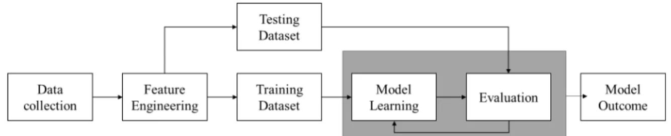
A traditional machine learning workflow (Figure 1) requires key constituents: data collection, feature engineering (cleaning and feature selection), model learning (training, validating and testing), and model evaluation [35].

10

Figure 1 Machine Learning Workflow

The collected raw data may be noisy, incomplete, or inconsistent, and before using the data as input in the model, it is required to pre-process it by removing errors and outliers and fill missing values. Other tasks include the integration of multiple datasets and transform the data into an appropriate format, so it is readable depending on the tool deployed to perform the machine learning process. Feature selection and extraction are utilized to reduce dimensionality in voluminous data, allowing to remove irrelevant or redundant features that promote over-fitting and to reduce computational requirements. Some techniques for dimension reduction include entropy, Fourier transform, and Principal Component Analysis (PCA) [35].

The training dataset is implemented to teach the model how to estimate the function that will be able to predict output for any new observation [33]. A validation dataset is applied to choose a suitable architecture for the model. If the architecture is pre-selected, there is no need for a validation set. Finally, the testing dataset allows the model to iterate and tune the different parameters until the model is ready to be deployed. The main decompositions of the dataset are 60/20/20% if training, validation, and test datasets or 70/30% if validation is not required [35]. The training data selection is relevant, because large, and accurate training datasets result in increased classification accuracy. It is being suggested that the minimum number of training samples should be ten or preferably 100 times the number of variables [34].

The evaluation focusses on the predictive efficacy of the model and on the computational requirements (training and testing time) for its application [36]. A high bias refers to a simple ML model that poorly maps the relations between features and outcomes (under-fitting) while a high variance implies an ML model that fits the training data but does not generalize well to predict new data (over-fitting) [35]. Techniques for experimental algorithm evaluation include bootstrap sampling, cross-validation, and holdout evaluation [36].

11 2.4.2 Supervised and Unsupervised Learning

Supervised learning uses labeled training datasets to create models, and typically, this approach is used to solve classification and regression problems [35]. Therefore, the algorithm uses patterns to predict the values of the labeled data on additional unlabeled data, and by comparing the actual output with the correct output, it finds the errors, learns, and modifies the model accordingly. Unsupervised learning uses unlabeled training datasets to create models that can discriminate between patterns in the data. This approach is most suited for clustering problems [35]. The algorithm explores the data and finds patterns for grouping together values based on their features.

2.4.3 Regression, Classification, and Clustering

In data clustering, the aim is to partition objects into groups such that similar objects are grouped while dissimilar objects are grouped separately. Categorical clustering views the data as a set of a two-dimensional matrix of data objects and attributes (a set of discrete values that are not comparable) and attempts to partition the set of objects into groups with similar attributes [36]. Well-known clustering algorithms are K-means and Kohonen Self-Organizing Maps (SOM). Whereas in classification and regression problems, the goal is to map a set of new input data to a set of discrete or continuous-valued outputs [35]. Some classification algorithms include Decision Trees (DT), Neural Networks (NN), K-Nearest Neighbors (k-NN), Bayesian Networks (BN), and Support Vector Machines (SVM). There are also ways of combining them into ensemble classifiers such as boosting, bagging, and the ensemble DT - Random Forest (RF). While known regression algorithms are mainly linear models such as Least Squares that include specific techniques such as OLS, MaxEnt, Logistic Regression [35], [36], LASSO Regression, SVM and Multivariate Regression algorithm.

2.4.4 Random Forest (RF)

Random Forest algorithm specifications for classification

The RF classifier is an ensemble classifier that uses multiple Classification and Regression Trees (CART) and combines their outputs to make a prediction, treating them as a “committee” of decision-makers [36], [37]. It combines the Bagging algorithm to reduce variance by the random selection of samples and the Random Subspace method to reduce bias by the random selection of the features employed at each split [36]. When operated for classification, each tree “votes” for a class and then classify using the “majority vote” of the forest [38]. Findings for Random Forest is that it does not overfit as more

12

trees are added, it is relatively robust to outliers and noise, gives useful internal estimates of error, strength, correlation and variable importance and is easily parallelized [37].

1. For b = 1 to B (n° of trees in the forest):

a. Draw a bootstrap sample Z* of the size N from the training data. b. Grow a random-forest tree 𝑇𝑇𝑏𝑏 to the bootstrapped data, by recursively

repeating the following steps for each terminal node of the tree, until the minimum node size

n

i. Select m variables at random from the p variables. ii. Pick the best variable/split-point among the m. iii. Split the node into two daughter nodes.

2. Output the ensemble of trees {𝑇𝑇𝑏𝑏}1𝐵𝐵.

To make a prediction at a new point x:

Classification: Let Ĉ𝑏𝑏(𝑥𝑥) be the class prediction of the bth random-forest tree. Then Ĉ𝑏𝑏𝑟𝑟𝑟𝑟𝐵𝐵 (𝑥𝑥) = majority vote {Ĉ𝑏𝑏(𝑥𝑥)}1𝐵𝐵.

Table 1 Algorithm: Random Forest for Classification [37], [38]

The first step in the RF algorithm in Table 1 (a) is to extract a “bootstrap sample” from the training dataset; bootstrapping allows to select the same sample more than once and include it in the subset dataset while other samples may not be selected at all. Bagging (acronym derived from Bootstrap AGGregatING) allows that each member of the ensemble is constructed from a different training set, each dataset being a bootstrap sample from the original [36]. About two-thirds of the samples (in-bag samples) are used to train the trees with the remaining one third (out-of-the-bag) are employed in an internal cross-validation technique for performance estimation of the model [37], [39].

Then, each tree is grown using samples from the bootstrapped dataset (b); however, it will select a random variable m from the full set of variables p available and pick the best one for the top split [38]. The random subspace principle is to increase diversity between members of the ensemble by restricting classifiers to work on different random subsets of the full feature space [36]. This procedure is repeated for the number of trees in the forest; bagging seems to enhance accuracy when random samples are utilized, this is also the case when using a single randomly chosen input variable to split on at each node [37].

13

Random forest classification of remote sensing datasets

ML algorithms have user-defined parameters that may improve classification accuracy when running parameter optimization. One of the benefits of the RF algorithm is that it is considered easy to optimize in comparison to more complex models such as ANN. Their stability concerning the choice of parameters makes them excellent candidates for operational processing chains, yielding classification accuracies as high as more sophisticated algorithms such as SVM but with much lower computational complexity [3].

RF has been exploited in time series analysis for creating multi-temporal cloud mask for Sentinel-2 imagery [30]; in supervised classification for producing land cover maps at a country scale for France [3], as well as crop type and land cover maps for Germany [24] and in global operational systems such as Sen2Agri for crop type maps [6].

RF algorithm requires only two user-defined parameters: the number of Decision Trees in the ensemble and the number of random variables at each node [34]. RF is computationally efficient and does not overfit [39]; the number of trees does not impact accuracy as long as it is large enough, being 500 a very conservative value [37]. The estimated error rate can be plotted for each ensemble size to determine when the performance stabilizes [34], [37].

Another advantage of RF is that the algorithm itself generates additional information [37]. The out-of-bag (OOB) error provides an unbiased estimate of generalization error and resembles the error estimate obtained by N-fold cross-validation [38]. Also, the Variable Importance (VI) estimation ranks the variables based on the predictive capabilities for discriminating between the target classes [37], [39]. The VI has been exploited in remote sensing to reduce the number of dimensions of hyperspectral data (i.e., the contribution of bands), to identify relevant ancillary data (i.e., topography) and to select the suitable season to classify target classes [34], [39]. This allows addressing the challenges of mitigating the Hughes phenomenon (i.e., the curse of dimensionality) that occurs when the number of variables is much larger than the number of training samples [39].

The main drawback is that it is sensitive to sampling design when imbalanced data is used; the final classification will under-predict the minority class [34]. To reduce misclassification, this sensitivity to sampling design needs to be considered by ensuring that training and testing are independent, establish balance and representativity of each class, and have an extensive training sample to deal with the number of data dimensions [39].

14

3 METHODOLOGY

The methodology section defines the study area (3.1), enumerates the datasets that were employed (3.2), and describes the methods implemented (3.3).

3.1 Study area

The Region of Interest (ROI) corresponds to the strata 214 in level 3 of the stratification of Continental Portugal (Figure 2). According to the classification, this area is about 1,223,890 ha in the low interior lands of the south of Portugal, which covers most of the valleys of the rivers Tejo and Sado and contains a great diversity of land uses as well as multiple crop types [40].

Figure 2 Stratification of Continental Portugal [40]. Scale 1:3,000,000.

This stratification considers the spectral diversity of the surface features, respective landcover, and geographic space [40]. When producing maps over large areas, stratification-based classification is recommended to avoid intra-class variability and has proven to yield better results for all the classification metrics than a tile-based approach [3].

15 3.2 Data

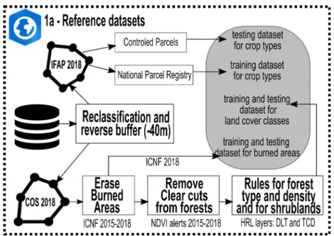
The research is based on the use of the ancillary data described in section 3.2.1, which allows the extraction of labeled points randomly; these serve as training data for producing a land cover and crop type map in raster format at 10m spatial resolution for 2018. The class nomenclature of the map is composed of 31 classes as can be appreciated in Table 2; the land cover classes like urban, forest and water are derived from the official LULC map of Continental Portugal (COS 2018) while the agriculture comprises annual and permanent crop as well as agricultural pastures obtained from the Land Parcel Identification System (LPIS) of the Instituto de Financiamento da Agricultura e Pescas (IFAP 2018), and finally, the burned areas are identified from the maps of the Institute for Nature Conservation and Forests (ICNF) from 2018. To avoid the inclusion of mislabeled pixels that can occur due to differences in the Minimum Mapping Unit (MMU) between datasets, the classes extracted were filtered with auxiliary information. These filters include the removal of burned areas (ICNF 2015-2018) and alerts based on the decrease of the Normalized Difference Vegetation Index (NDVI) between two dates acquired from Landsat 8 imagery (2015-2018); allowing to remove potential clear cuts [17]. Likewise, the Copernicus High-Resolution Layers (HRL) datasets from 2015 (latest available), particularly Dominant Leaf Type (DLT) and Tree Cover Density (TCD), is used distinguish between forest types, forest density and to eliminate non-forest pixels. All the previous datasets mentioned were provided by DGT, including the simplified COS nomenclature (COSsim) in Table 2 that is under constant improvements for the foRESTER project. The editable version of the Land Cover and Crop Type nomenclature and corresponding RGB color scheme to symbolize the different classes can be found in annexes 7.2 and 7.3, respectively.

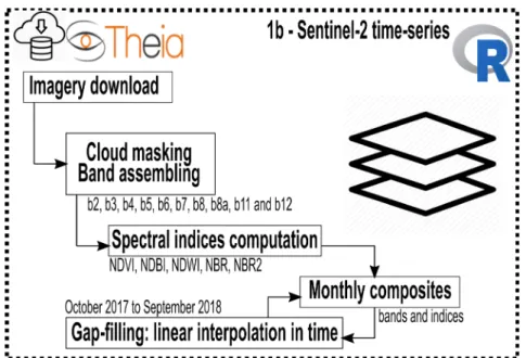
Also, a crucial input in this research is the intra-annual time series of Sentinel-2a and b from ESA for the period of October 2017 to September 2018 3.2.2. It is fundamental to mention that all the procedures in section 3.3.3, namely acquisition and pre-processing, indices calculation, production of monthly composites and filling of missing values was done by Hugo Costa and Pedro Benevides under the IPSTER project at DGT, using the R software and the computer specifications provided in section 3.3.1.

16 3.2.1 Ancillary data

The ancillary data used as a reference for training and validating, as well as the filters applied to preprocess the reference datasets, is described in this section.

COS 2018

The official LULC of Continental Portugal (COS) is a vectorial map with an MMU of 1 hectare, a minimum distance between lines of 20m and produced through visual interpretation of orthophoto maps (25 cm pixel size) and auxiliary data. Each polygon contains only one LCLU code selected from the most detailed hierarchical level of the nomenclature, and this class must occupy equal or more than 75% of the entire delimited area. The COS 2018 contains a total of 83 classes in the fourth level of detail (LV4) that can be aggregated to a first level (LV1) containing 9 LCLU mega classes such as artificialized territories, agriculture, pastures, agroforestry surfaces, forests, open spaces or with sparse vegetation, wetlands, and surface water masses. As an example, in section 7.3 the Cork Oak forest in LV3 corresponds to a Broadleaf forest in LV2 and to the mega class Forests in LV1. The technical specifications are available in the official documentation of COS 2018 for Continental Portugal [7].

The version under current development COS2018v1 is the one being used; therefore, some nomenclatures might change during the writing of this document. A total of 16 LC classes were derived from the 83 classes available in LV4 of the COS nomenclature; all of them will be used for training and testing as it can be appreciated in Table 2, the classes from COS 2442 (Holm oak agroforestry system) and class 3112 (pure forest of Holm oak) were combined into the class 5121 (Holm oak forest) as both represent the same LC but have different uses. The class 6111 corresponding to shrubland corresponds to areas that remained shrubland through the COS series, meaning that shrubland was present in 1990, 1995, 2007, 2010, 2015 and 2018.

IFAP 2018

The Portuguese Land Parcel Identification System (LPIS) of the Instituto de Financiamento da Agricultura e Pescas (IFAP) is comprised of two independent datasets. The “national parcel registry” that will be used for training and the “controlled parcels” for testing. The first consists of the parcels reported by the farmers that applied for agricultural subsidies in the frame of CAP. The second dataset is the controlled parcels containing polygons with rectified edges through the visual interpretation of orthophotos

17

and field verification to assess the crop type planted. Overall, the LPIS is a very reliable product used in countrywide crop mapping studies; however, it can contain errors such as false claims or digitization errors [24].

The IFAP 2018 is composed of more than 175 types of crops, mapping such a number of classes at 10 m resolution can be challenging. Instead, the ten most abundant temporary crops (5 rainfed and 5 irrigated), three permanent crops, and the agricultural grasslands were selected for the analysis for a total of 14 crop types classes.

The IFAP also provides a crop calendar (in attachment 7.3) that illustrates the growing period for the crops monitored in Portugal. The early stages of the crops correspond to the flooding-only for rice-, seed, and crop development (germination and tillering) where the area is not covered yet by the vegetation. Then, the peak of greenness occurs during the flowering, fruit, and ripening. Finally, during the harvest, depending on the farmer's practices, the soil can remain clear, with stubble or left to natural regeneration.

Burned areas (ICNF 2015-2018)

The Institute for Nature Conservation and Forests (ICNF) is responsible for the realization of an annual map of burned areas for Portugal based on visual interpretation of Landsat TM/ETM. The institute publishes on its website at the end of each fire season a vectorial dataset containing burned areas larger than five hectares [17], [41]. The polygons used contains the information for the areas that burned by wildfires during the years 2015 to 2018.

After a wildfire, it is likely that the LC type changes, as forest and shrubs, would not be present anymore in scorched areas. The ICNF mask is implemented as the first filter for the COS dataset to avoid extracting samples of vegetation from burned areas. This allowed erasing the pixels that correspond to grasslands, forests, or shrubland classes in COS 2018 but fall inside the burned areas. Whereas the year 2018 was used to extract training and testing points for this class, corresponding to the last class in the nomenclature.

18 NDVI mask

Furthermore, it is not possible to sample broadleaf or coniferous forests from areas where trees have been uniformly cut down (i.e., clear cuts). According to Costa et al. (2018) [17], land cover changes can potentially be detected by monitoring if the inter-annual values of NDVI decrease between two successive years over a certain threshold. Therefore, the NDVI mask (derived from Landsat 8) can help to identify clear cuts in a forest, allowing to exclude these areas from the training samples for broadleaf or coniferous forests in COS 2018.

High-Resolution Layers (HRL 2015)

Delivered at a Pan-European level, the HRL is a product available in the Land Monitoring Service of Copernicus. These layers are complementary to the production of CLC, and it is available for continental Portugal [42]. The HRL for the thematic class forest of 2015 was used in the preprocessing of forests and shrublands of COS 2018. Two of the forest products are used, the Tree Cover Density (TCD) representing the percentage that a pixel is covered by trees and Dominant Leaf Type (DLT) that allows distinguishing between broadleaf or coniferous majority.

20

21 3.2.2 Remote Sensing Data

Sentinel 2

The Copernicus Sentinel-2 mission is a constellation of two polar-orbiting satellites that operate simultaneously, phased at 180° to each other at a mean altitude of 768 km. This allows a and high revisit time (10 days for S2-A and 5 days for S2A/B), and its wide swath width (290 km) provides a high coverage [43] being ideal for the proposed study. The imagery is acquired by the Multispectral Instrument (MSI) on-board Sentinel-2 and contains 13 spectral bands from Visible/Near Infrared (VNIR) to Short Wave Infrared (SWIR) and comes in three spatial resolutions (10, 20 and 60m) as seen in Table 3.

Band Spatial

resolution (m) Central wavelength(nm) Bandwidth (nm) Purpose

B01 60 443 20 Aerosol detection B02 10 490 65 Blue B03 10 560 35 Green B04 10 665 30 Red B05 20 705 15 Red Edge B06 20 740 15 Red Edge B07 20 783 20 Red Edge

B08 10 842 115 Near Infrared (NIR)

B08A 20 865 20 NIR B09 60 945 20 Water vapor B10 60 1375 30 Cirrus B11 20 1610 90 Snow/ice/cloud discrimination (SWIR) B12 20 2190 180 Snow/ice/cloud discrimination (SWIR) Table 3 Specifications of the Sentinel-2 bands

The Sentinel-2 data was obtained from the French Theia Land Data Centre (THEIA). The data is in the Coordinate Reference System (CRS) of Universal Transverse Mercator (UTM) Zone 29N, and it is tiled in the Military Grid Reference System (MGRS) allowing all the images to have the same size (100x100 km2) and a code (e.g., a tile in Portugal is T29SND).

22

The biogeographical region 214 “Tejo and Sado” is covered by four tiles of Sentinel-2 that correspond to 29SNB, 29SNC, 29SND, and 29SPD. The classification will be done for the strata 214 that is within the tiles 29SNC and 29SND. Most of the study area is comprised within the same orbit; however, a slight corner in the 29SND tile has swath overlap with the adjacent orbit, accounting for more imagery collected within the same period than tile 29SNC. Although the re-visitation period is the same, the dates in the collection of the orbits vary from left to right in adjacent land.

Figure 3 Sentinel-2 orbit, swath, and tilling for the study area and images acquired for October 2017 in the tile 29SND.

Orthophotos for Continental Portugal

For all the visualizations, the orthophotos available as Web Map Service (WMS) from DGT were used. The imagery has a spatial resolution of 25 cm, and it is available for Continental Portugal.

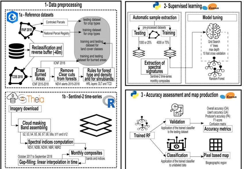
23 3.3 Methods

The proposed methodology corresponds to an automatic supervised classification procedure using the random forest classifier, intra-annual time-series of Sentinel-2, and filtered auxiliary data to extract the labels for land cover and crop types automatically (Figure 4). First, the reference datasets (COS2018 and IFAP 2018) are reclassified using the nomenclature from, then a set of preprocessing rules is applied to the datasets to remove the pixels that do not match the class label (3.3.2).

Next, section 3.3.3 illustrates the preprocessing of the Sentinel-2 intra-annual time series. Initially, the imagery is downloaded for the period of October 2017 to September 2018; a mask to remove clouds and cloud shadows are applied, and all the bands are resampled to 10m. Later, five spectral indices are calculated, and all the imagery is aggregated to monthly composites. The potential missing values (pixels with no data during a month) are filled using linear interpolation in time to ensure continuity of information during the period.

Afterward, the supervised learning procedure is presented in section 3.3.4. This section starts with the automatic extraction of samples by class from the pre-processed datasets. Two independent sample datasets are acquired, one for training and one for testing with varying percentages 80/20 or 75/25 depending on the number of pixels available. For each sample, the spectral signatures are retrieved at the pixel level from all the bands of the composites and the spectral indices. Then, a grid search is used to determine the best hyperparameters for the RF; the models are fit to the training dataset and assessed with 10-split cross-validation.

At last, the performance of the best model is quantified following the metrics in (3.3.5) based on the predicted labels in the testing dataset. Then, the model is applied to unlabeled data allowing to generate the final map for the biogeographical region.

24

25 3.3.1 Software and device specifications

The data pre-preprocessing was done using the software ArcGIS Pro 2.4.0 from ESRI. A geoprocessing workflow was developed with the visual programming language of Model Builder that can later be exported as a python script.

The sample extraction, model training, and classification were done using Anaconda Distribution that is an open-source platform to perform data science and machine learning. The version installed corresponds to Anaconda3-4.4.0-Windows-x86_64 that contains Python (3.5.4) and the required libraries such as NumPy (1.13.1) [44] and Pandas (0.20.3) [45] for data structures, Seaborn and Matplotlib (2.0) [46] for data visualization and Scikit-Learn [47] for conducting machine learning analysis since it includes the random forest classification algorithm. Other libraries installed comprise GeoPandas for its spatial functionality with geospatial data and the Geospatial Data Abstraction Library (GDAL), which is a translator library for raster and vector geospatial data formats [48].

The feature extraction, classification, and the elaboration of the final map were done using the computers of DGT. The computers have an installed RAM of 64.0 GB with a processor Intel (R) Xeon (R) Gold 6140 CPU @ 2.3GHz 2.29 GHz. For all the other procedures, a personal computer was used, with a processor Intel (R) Core (TM) i7-7500U CPU @ 2.70 GHz 2.90 GHz and installed RAM of 8.00 GB.

3.3.2 Preprocessing of the reference datasets

The workflow for pre-processing the reference datasets is detailed in Figure 5. First, the IFAP 2018 dataset was reclassified from 175 crop types to 14, and a buffer of -40m was applied. Next, from the 83 classes available in COS 2018 dataset, a total of 15 were extracted; likewise, an inner buffer was used. Then, the remaining polygons were crossed with the auxiliary data; this includes the ICNF burned areas 2015-2018, NDVI alerts of clear cuts 2015-2018, and HRL layers 2015 (DLT and TCD). Finally, if IFAP had overlapping areas with COS, these were removed from the latter; the final dataset comprises IFAP 2018, COS 2018 and ICNF 2018. As the IFAP controlled parcels were used for testing while the national parcel registry was used for training, both datasets were kept spatially independent. This is not the case for COS nor ICNF, being the whole dataset used both for training and testing.

26

Figure 5 Data preprocessing workflow for reference datasets

Crop type dataset (IFAP 2018)

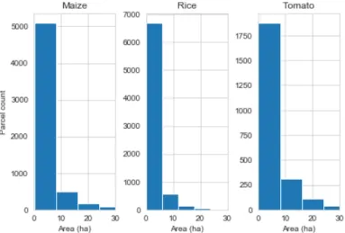
From the IFAP dataset, the ten most abundant temporary crops (5 rainfed and 5 irrigated), three permanent crops, and the agricultural grasslands were selected for the analysis for a total of 14 crop types classes. An Exploratory Spatial Data Analysis (ESDA) was performed to identify the ten most abundant temporary crops in the study area for the classification (Figure 6); these corresponds to maize (24,012ha), rice (21,595 ha), tomato (12,742ha), ryegrass (5,472ha), oatmeal (4,163ha), wheat (2,723ha), sorghum (2,104ha), barley (1,844ha), lupin (1,762ha) and potato (1,748ha). As for the permanent crops, olive trees, vineyards, and orchards were considered due to their importance in Portugal’s agriculture. The orchard class combines 17 types of trees from figs and oranges to walnuts and hazelnuts.

27

The number of parcels is relevant; the more parcels are distributed within the study area, the more representativity is possible to obtain. According to the distribution of the parcels (Figure 7), most of them are less than 10 ha. The average area for all the classes is 3.35 ha, being the tomato parcels with the higher mean area (5.38ha) and oatmeal the lower mean area (2.35ha).

Figure 7 Distribution of the tree main crop parcels by area (ha)

An inverse buffer of -40 m was performed to the original parcels to avoid selecting pixels for which the spectral signature does not match the class label, as can be seen in Figure 8. During the buffering process, it can occur that the smallest parcels are removed from the dataset, reducing the number of available pixels for training. No other crossing with ancillary data was applied to this dataset, training (national parcel registry) and testing (controlled parcels) were kept independent. This was ensured by performing an intersection between the datasets and removing the controlled parcels from the national parcel registry guaranteeing that all the polygons are spatially disjointed.

28 Land Cover dataset (COS 2018)

A total of 16 LC classes were derived from the 83 classes available in COS 2018, and a -40 m buffer was applied to the remaining polygons. Yet, it is critical to emphasize that the MMU of COS (1ha) entails a reduction in detail to better model the reality; and many times, it requires the generalization of polygons. This means that areas smaller than 1ha (paths, edifications and other objects) will be aggregated with the predominant class up to 25% of the total area of the polygon [7]. Classification at the pixel level for Sentinel-2 contemplates a 10 m MMU; therefore, some pre-processing steps are required to prevent the selection of pixels with spectral information that mismatch the class label inherited from COS which has a larger MMU (and potential thematic errors).

The first step was to intersect all COS polygons with the ICNF burned mask for the years 2015- 2018. The mask allowed to create holes in the polygons by eliminating the scorched areas; consequently, no automatic sample will be extracted from these areas. A total of 392 ha in 2015, 2565 in 2016, 6002 ha in 2017, and 99 ha in 2018 were removed from the dataset. In Figure 9, it is possible to recognize a blackened area inside a Maritime Pine class in 2016 and inside a Eucalyptus class in 2017. Still, the burned mask does not cover the polygon extensively, as it can be appreciated in the Maritime pine where two holes remained in the polygon corresponding to edifications and in Eucalyptus where the mask does not cover the total extent of the area. The forest type most reduced in the area after applying by the burned mask correspond mainly to cork oak (263 772 ha) and eucalyptus (80 323 ha). In Portugal, the eucalyptus forest is industrially grown to supply pulp fiber for the paper industry, although they are highly flammable [49].

29

Figure 9 COS2018 polygon overlaid with the burned mask, Maritime Pine OBJECTID: 493848 and Eucalyptus OBJECTID: 415864. Scale 1:7,000 (1) and 1:25,000 (2).

The second step applies only for the forest areas since training and testing cannot be sampled from forest cuts. NDVI differencing techniques allow discriminating between real changes and seasonal or inter-annual variability of forests [50]. This technique has been implemented in Portugal [51] to detect vegetation loss that occurred between 2015-2018 in forests, so-called NDVI alerts. The forest polygons were crossed with the NDVI alerts mask to remove the areas where there have been changes, and hence the class label of COS does not correspond to the pixel spectral signature. After applying the mask, the most affected forests are eucalyptus with 13785 ha reduced, followed by 7076 ha in stone pine and 3498 ha in maritime pine. This forest fragmentation (i.e., breaking of large, contiguous forested areas into smaller pieces of a forest) is due to some extent to road construction, fires, logging and conversion to agriculture. In the case of forest plantations like eucalyptus, clear-cuts are part of the forest management cycle; as a new forest is expected to follow, the land use remains a forest [51]. However, in a strictly land cover map derived from supervised classification, these changes in vegetation can result in misclassifications when implementing the model and therefore require to be removed from sample extraction.

Figure 10 NDVI alerts in a Eucalyptus plantation (COS 2018 OBJECTID: 382944). Scale 1:80,000 (1) and 1:6,000 (2).

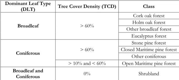
The final step was to cross the forest areas, and the shrublands with the High-Resolution Layers (HRL) masks created following the rules in Table 4. The Dominant Leaf Type (DLT) allows separating broadleaf or coniferous majority, while the Tree Cover Density (TCD) ranges from 0 to 100%. For cork oak, holm oak, other broadleaf, and eucalyptus, it is required that they correspond to broadleaf with a tree cover higher than 60% of the pixel in the HLR. For coniferous, if more than 60% of the pixel is covered by

30

trees, then the classes stone pine and other coniferous are defined. However, for the class maritime pine, if the coverage is more than 60%, it is considered a closed maritime pine. Although, if the pixel coverage is between 10% and 60%, a new class is derived, and it is considered an open maritime pine. A shrub is a type of vegetation that is included in many classes as a percentage in the area, making it challenging to identify. For the shrubland class, the rule is to remove from the class all the areas with broadleaf or coniferous cover.

Dominant Leaf Type

(DLT) Tree Cover Density (TCD) Class

Broadleaf > 60%

Cork oak forest Holm oak forest Other broadleaf forest

Eucalyptus forest

Coniferous > 60%

Stone pine forest Closed Maritime pine forest

Other coniferous > 10% and < 60% Open Maritime pine forest Broadleaf and

Coniferous 0% Shrubland

Table 4 Rules for the crossing of COS polygons with HRL

Following the application of the mask, there is a dramatic reduction in the area for all the classes. Cork oak presented the highest reduction of 260000 ha, followed by eucalyptus with 64000 ha and stone pine with 51000 ha. Figure 11 exemplifies the filtering using the HRL layers in shrubland. It is possible to visualize that the areas with broadleaf and forest containing more than 0% of tree cover density are masked out the shrubland polygon.

Figure 11 DLT (1) and TCD (2) rule for shrublands (COS OBJECTID: 592293). Scale 1:20,000.

31

At last, all the polygons within classes must be mutually exclusive; therefore, the polygons from the IFAP dataset were intersected with the polygons from COS. The overlapping areas were erased from the COS land cover dataset, giving priority to IFAP. When removing the areas that overlapped between IFAP and COS dataset, a significant conversion from land cover to crop types were found. Three main classes were reduced in the area: 114 ha of natural grassland, 72ha of open maritime pine, and 121ha of cork oak were reclassified to agriculture.

3.3.3 Preprocessing of the intra-annual time series of Sentinel 2

The following descriptions are summarized from the technical specifications for the generation of multi-temporal Sentinel-2 composites for mainland Portugal [52]. The workflow includes acquisition and preprocessing, indices computation, generation of the monthly composites, and filling of missing values, as illustrated in Figure 12.

Figure 12 Preprocessing workflow for Sentinel-2 intra-annual time series

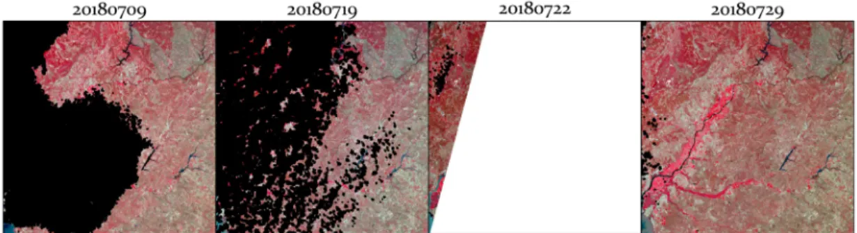
Acquisition and preprocessing

The Sentinel-2 images downloaded from THEIA for the agricultural year of 2018 comprise a cloud coverage < 50%, each tile contains around 81 images and occupy 51 GB per tile. The THEIA images available for download are already pre-processed with an algorithm named MAJA and have a more efficient cloud masking algorithm when compared with the original ESA Sen2Cor Sentinel-2 processor [30]. The MAJA algorithm provides atmospheric correction to the bottom of the atmosphere (BOA), a mask for