Clustering for Decision Support in the Fashion Industry
Ana Lisa Amorim do Monte
Orientação: Prof. Dr. Carlos Soares
Co-orientação: Prof. Dr. Pedro Brito
Dissertação de Mestrado em Economia e
Administração de Empresas
CLUSTERING FOR DECISION SUPPORT IN THE
FASHION INDUSTRY
por
Ana Lisa Amorim do Monte
Dissertação de Mestrado em Economia e Administração de Empresas
Orientada por
Prof. Dr. Carlos Soares
Co-orientada por
Prof. Dr. Pedro Quelhas Brito
III
Nota Biográfica
Ana Lisa Amorim do Monte nasceu a 8 de Novembro de 1981 na cidade da Póvoa de Varzim. Licenciou-se em Gestão na Faculdade de Economia da Universidade do Porto (FEP) em 2005. Durante o curso participou no 44th European Congress of European Regional Science Association (ERSA) como Assistente em 2004.
Após ter terminado a licenciatura, iniciou em 2006 um estágio profissional do IEFP na empresa Monte-SGPS, S.A. na Póvoa de Varzim na área de gestão. Concluído o estágio em 2007, ingressou durante um período de 2 anos no Banco Popular Portugal, S.A., onde executou funções de Caixa e de Gestor de Clientes Particulares numa das suas agências em Portugal. Foi durante a sua permanência no banco, que decidiu integrar o Mestrado em Economia e Administração de Empresas na FEP, tendo iniciado no ano lectivo 2009/2010.
Em 2009, finda a sua passagem pela área da banca, ingressa numa experiência internacional. Participa no Programa de Estágios Internacionais da AICEP, o “Inov Contacto”, através do qual colabora, durante um período de seis meses, com a empresa Sonae Sierra, nos seus escritórios localizados em Atenas na Grécia, na área de Reporting Operacional.
Terminado esse estágio internacional em 2010, regressa a Portugal e nesse mesmo ano inicia um estágio interno, com duração de um ano, no Shared Service Center da empresa alemã Infineon Tecnologies, situada no TECMAIA - Parque de Ciência e Tecnologia da Maia - onde integra o departamento de Accounts Payable.
Em finais de 2011, terminado esse estágio interno, a sua dedicação focou-se na finalização do Mestrado, tendo já concluído a parte curricular.
V
Agradecimentos
Este trabalho só foi possível realizar através da colaboração e incentivo de um conjunto de pessoas e entidades.
Agradeço ao meu orientador, o Professor Doutor Carlos Manuel Milheiro de Oliveira Pinto Soares, pela atenção, disponibilidade, simpatia, dinamismo, sentido crítico construtivo e acima de tudo pela confiança que depositou neste projecto e na minha pessoa.
Ao meu co-orientador, o Professor Doutor Pedro Manuel dos Santos Quelhas Taumaturgo de Brito, que aceitou contribuir neste projecto com a sua preciosa ajuda e disponibilidade e com os seus incontestáveis conhecimentos na área que mais domina.
Ao LIAAD - Laboratory of Artificial Intelligence and Decision Support, unidade associada do INESC TEC - INESC Tecnologia e Ciência, que me acolheu simpaticamente cedendo o seu espaço e meios para poder realizar este trabalho.
À empresa Bivolino que disponibilizou os seus dados que serviram de base em todo este trabalho, pela sua contribuição e simpatia.
The research leading to these results has received funding from the European Union Seventh Framework Programme (FP7/2007-2013) under grant agreement n° 260169 (Project CoReNet - www.corenet-project.eu).
A todos os meus amigos e colegas, à minha família e ao meu namorado que sempre me apoiaram e incentivaram a não desistir e lutar pelos meus objectivos, que sempre me fizeram acreditar nas minhas capacidades.
VII
Resumo
O tema deste trabalho é a segmentação das encomendas de uma empresa belga, a Bivolino, cuja actividade se foca essencialmente na comercialização de camisas feitas à medida de cada cliente. Essa segmentação é feita com a ajuda de técnicas de Data Mining, tendo sido utilizada neste trabalho a técnica de Clustering, a qual é considerada uma das mais importantes técnicas de Data Mining. Esta técnica faz a partição dos dados de acordo com um dado critério de similaridade ou distância, sendo a Distância Euclidiana o mais comummente utilizado.
O método de Clustering seleccionado para fazer a partição dos dados foi o K-Medoids, dado este ser menos sensível a outliers do que outros métodos e principalmente por poder lidar com dados nominais. A computação deste método foi realizada com recurso a um software para Data Mining, o chamado RapidMiner. Das várias experiências efectuadas com os dados no RapidMiner, foram seleccionados os resultados que seriam objecto de análise e interpretação quer numa perspectiva técnica quer numa perspectiva de Marketing.
Os resultados mostram que é possível identificar as tendências de moda nas camisas da Bivolino para apoiar as decisões da empresa a nível do Design e do Marketing. Este trabalho contribui para demonstrar a potencialidade da utilização de ferramentas de Data Mining para analisar grandes quantidades de dados de empresas transformando-os em informação útil e daí extraírem conhecimento acerca do seu negócio. Será esse conhecimento que lhes vai permitir tomar importantes decisões em tempo útil e obter vantagens competitivas.
Palavras-chave: Data Mining, Clustering, K-Means, K-Medoids, Marketing,
IX
Abstract
The scope of this work is the segmentation of the orders of a Belgian company, named Bivolino, which sells custom tailored shirts. The segmentation was done with the help of Data Mining techniques, namely Clustering. Clustering is considered one of the most important Data Mining techniques. Its goal is to partition the data according to some similarity/distance criterion, where the most commonly used is the Euclidian Distance.
In this study, we used the K-Medoids clustering method, because it is less sensitive to outliers than other methods and it can handle nominal variables. The Data Mining software used was RapidMiner. Out of the many experiments that were carried out a few results were selected to be then analyzed and interpreted from technical and Marketing perspectives.
The results show that it is possible to identify fashion trends in Bivolino shirts to support the decisions of the company concerning Design and Marketing. This work provides further evidence of the potential of Data Mining tools to analyze large amounts of business data. The results of this analysis is useful knowledge from which companies can extract regarding their business. This knowledge will allow those companies to make important business decisions in time and, thus, obtain competitive advantages.
Keywords: Data Mining, Clustering, Cluster, K-Means, K-Medoids, Marketing,
XI
Table of Contents
Nota Biográfica ... III Agradecimentos ... V Resumo ... VII Abstract ... IX List of Tables... XV List of Figures ... XVII Abbreviations ... XIX
PART I ... 1
1. INTRODUCTION ... 3
1.1. Structure ... 4
2. DATA MINING ... 6
2.1. Data Mining Definition ... 7
2.2. Data Mining Tasks ... 8
2.3. Data Mining Process ... 9
2.3.1. Identify the Business Opportunity ... 9
2.3.2. Transform Data using Data Mining Techniques ... 10
2.3.3. Take Action ... 10
2.3.4. Measure the Results ... 10
2.4. Data Mining Methodology ... 11
2.4.1. Hypothesis Testing ... 11
2.4.2. Knowledge Discovery... 11
2.4.2.1. Directed Knowledge Discovery ... 12
2.4.2.2. Undirected Knowledge Discovery ... 12
3. CLUSTERING ... 13
3.1. Clustering Definition... 13
3.2. Clustering Goals ... 14
XII 3.4. Clustering Algorithms ... 15 3.4.1. K-Means Clustering ... 17 3.4.2. K-Medoids Clustering... 20 3.5. Cluster Validity ... 21 4. SEGMENTATION IN MARKETING ... 27 4.1. Segmentation Definition ... 27 4.2. Segmentation Effectiveness... 27 4.3. Segmentation Process ... 29
4.4. Levels of Market Segmentation ... 30
4.4.1. Mass Marketing ... 31
4.4.2. Segment Marketing... 31
4.4.3. Niche Marketing ... 31
4.4.4. Micro Marketing ... 32
4.5. Segmentation Bases ... 32
4.5.1. Observable General Bases ... 33
4.5.2. Observable Product-Specific Bases ... 33
4.5.3. Unobservable General Bases ... 33
4.5.4. Unobservable Product-Specific Bases ... 34
4.6. Segmentation Methods ... 35
4.6.1. A Priori Descriptive Methods ... 36
4.6.2. Post Hoc Descriptive Methods ... 36
4.6.3. A Priori Predictive Methods ... 36
4.6.4. Post Hoc Predictive Methods ... 37
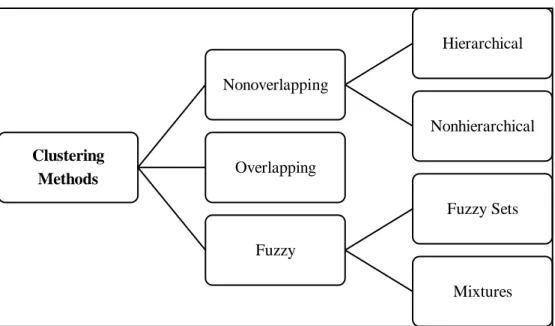
4.7. Segmentation Methodology – Clustering Methods ... 38
4.7.1. Non-overlapping Methods ... 40
4.7.2. Overlapping Methods ... 41
4.7.3. Fuzzy Methods ... 41
PART II... 43
5. RESULTS ANALYSIS IN A TECHNICAL PERSPECTIVE ... 45
XIII
5.2. Interpretation of Clusters ... 46
5.3. Conclusions of the Clustering Results ... 65
6. RESULTS ANALYSIS IN A MARKETING PERSPECTIVE ... 67
6.1. Identification of Segments... 67
6.2. Identification of Segmentation Variables ... 70
6.3. Interpretation of Segments ... 73
6.4. Conclusions of the Results ... 91
7. CONCLUSION ... 97
7.1. Summary ... 97
7.2. Recommendations ... 99
7.3. Limitations of the Study ... 100
7.4. Future Work ... 101 APPENDICES ... 103 APPENDIX A ... 105 APPENDIX B ... 109 ANNEXES ... 129 ANNEX A ... 131 ANNEX B ... 139 ANNEX C ... 143 ANNEX D ... 145 ANNEX E ... 153 ANNEX F ... 157
XV
List of Tables
Table 2.1 – Data Mining Tasks...8
Table 3.1 – Clustering Perspectives...13
Table 3.2 – K-Means: Common choices for proximity, centroids and objective functions...19
Table 3.3 – Selected Distance Functions between Patterns x and y...20
Table 3.4 – Internal Validity Indices...22
Table 3.5 – External Validity Indices...24
Table 4.1 – Requirements for an Effective Segmentation...28
Table 4.2 – Steps in Segmentation Process...29
Table 4.3 – Levels of Marketing Segmentation...30
Table 4.4 – Classification of Segmentation Bases...32
Table 4.5 – Evaluation of Segmentation Bases...34
Table 4.6 – Classification of Segmentation Methods...35
Table 4.7 – Evaluation of Segmentation Methods...37
Table 5.1 –Shirts Attributes Values of Cluster 1...47
Table 5.2 – Representation of Binominal Attributes...54
Table 5.3 – Shirts Attributes Values of Cluster 2...55
Table 5.4 – Similarities against Cluster 1...56
Table 5.5 – Shirts Attributes Values of Cluster 3...57
Table 5.6 – Similarities against Cluster 1 and Cluster 2...58
Table 5.7 – Shirts Attributes Values of Cluster 4...59
Table 5.8 – Similarities against Cluster 1, Cluster 2 and Cluster 3...60
Table 5.9 – Shirts Attributes Values of Cluster 5...61
Table 5.10 – Similarities against Cluster 1, Cluster 2, Cluster 3 and Cluster 4...62
Table 5.11 – Shirts Attributes Values of Cluster 6...63
Table 5.12 – Similarities against Cluster 1, Cluster 2, Cluster 3, Cluster 4 and Cluster 5...64
Table 6.1 – Representation of Distinct Attributes Values of Segment 2...69
Table 6.2 –Representation of Bivolino Orders by Gender...69
Table 6.3 – Classification of Segmentation Variables...72
XVI
Table 6.5 – Obesity of Male Customers measured by the Collar Size...77
Table 6.6 – Obesity of Male Customers...78
Table 6.7 – Bivolino Gift Vouchers Usage analysis...79
Table 6.8 – Customers Attributes Values of Segment 2...80
Table 6.9 – Obesity of Female Customers measured by the Collar Size...84
Table 6.10 - Obesity of Female Customers...84
Table 6.11 - Customers Attributes Values of Segment 3...85
Table 6.12 - Similarities against Segment 1...85
Table 6.13 - Customers Attributes Values of Segment 4...86
Table 6.14 - Similarities against Segment 1 and Segment 3...87
Table 6.15 - Customers Attributes Values of Segment 5...88
Table 6.16 - Similarities against Segment 1, Segment 3 and Segment 4...88
Table 6.17 - Customers Attributes Values of Segment 6...90
XVII
List of Figures
Figure 2.1 – The four stages of Data Mining Process...9
Figure 3.1 – Hierarchical Clustering...16
Figure 3.2 – Partitional Clustering...16
Figure 3.3 – A Taxonomy of Clustering Approaches...16
Figure 3.4 – K-Means Clustering Steps...18
Figure 3.5 – K-Means algorithm Process...19
Figure 3.6 – A Simplified Classification of Validation Techniques...26
Figure 4.1 – Levels of Marketing Segmentation...30
Figure 4.2 – Classification of Clustering Methods...39
Figure 4.3 – Clustering Methods: (a) nonoverlapping, (b) overlapping, (c) fuzzy...39
Figure 4.4 – Nonoverlapping Hierarchical Clustering Methods...40
Figure 5.1 – Result of K-Medoids Clustering Extract Cluster Prototype for k=6...45
Figure 5.2 – Representation of Cluster 1...46
Figure 5.3 – Illustration of Designing a Men Shirt on Bivolino website – Shirt attributes...48
Figure 5.4 – Illustration of Designing a Men Shirt on Bivolino website – Customers attributes...49
Figure 5.5 – Fabrics of Men Shirts...49
Figure 5.6 – Fabric Colors of Men Shirts...50
Figure 5.7 – Fabric Design and Pattern of Men Shirts...50
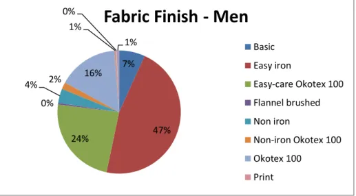
Figure 5.8 – Fabric Finish of Men Shirts...51
Figure 5.9 – Fabric Structure of Men Shirts...51
Figure 5.10 – Fabric Material of Men Shirts...52
Figure 5.11 – Collar of Men Shirts...52
Figure 5.12 – Cuff of Men Shirts...53
Figure 5.13 – Placket of Men Shirts...53
Figure 5.14 – Hem of Men Shirts...54
Figure 5.15 – Representation of Cluster 2...55
Figure 5.16 – Representation of Cluster 3...57
Figure 5.17 – Representation of Cluster 4...59
XVIII
Figure 5.19 – Representation of Cluster 6...63
Figure 6.1 – Result of K-Medoids Clustering Extract Cluster Prototype for k=6 with extra variables...67
Figure 6.2 – Representation of Segment 1...73
Figure 6.3 – Representation of Men Orders by country...74
Figure 6.4 – Age Groups of Male Customers...74
Figure 6.5 – Height Groups (in cm) of Male Customers...75
Figure 6.6 – Weight Groups (in kg) of Male Customers...75
Figure 6.7 – BMI measures of Male Customers...76
Figure 6.8 – Collar Groups of Male Customers...77
Figure 6.9 – Representation of Segment 2...78
Figure 6.10 – Bivolino Gift Vouchers...80
Figure 6.11 – Representation of Women Orders by Country...81
Figure 6.12 – Age Groups of Female Customers...81
Figure 6.13 – Height Groups (in cm) of Female Customers...82
Figure 6.14 – Weight Groups (in kg) of Female Customers...82
Figure 6.15 – BMI measures of Female Customers...83
Figure 6.16 – Collar Groups of Female Customers...83
Figure 6.17 – Representation of Segment 3...84
Figure 6.18 – Representation of Segment 4...86
Figure 6.19 - Representation of Segment 5...87
Figure 6.20 - Relation between Age and BMI for Male Customers...89
Figure 6.21 - Representation of Segment 6...89
Figure 6.22 - Relation between Country and Affiliate for Male customers...91
Figure 6.23 - Relation between Fit and Age for Male Customers...92
Figure 6.24 - Fit choices of Men Shirts...92
Figure 6.25 - Relation between Pocket and Age for Male Customers...93
Figure 6.26 - Type of Pocket for Men Customers...93
Figure 6.27 - Total Orders by Country of Bivolino Shirts in 2011...94
XIX
Abbreviations
AID – Automatic Interaction Detection ANN – Artificial Neural Network BMI – Body Mass Index
CART – Classification and Regression Trees
CHAID – AID for Categorical Dependent Variables
CRISP-DM – Cross Industry Standard Process for Data Mining DM – Data Mining
KD – Knowledge Discovery
PART I
“Theory helps us to bear our ignorance of facts.”
3
1. INTRODUCTION
“There are no secrets to success. It is the result of preparation, hard work, and learning from failure.”
By Colin Powell, an American statesman
This dissertation is focused on the problem of supporting fashion industry in its production/design and marketing decisions based on Data Mining (DM) approaches. Short life cycles, high volatility, low predictability, and high impulse purchasing is being appointed has characteristics of fashion industry (Lo et al, 2008).
The data that companies collect about their customers is one of its greatest assets (Ahmed, 2004). However, companies increasingly tend to accumulate huge amounts of customer data in large databases (Shaw et al, 2001) and within this vast amount of data is all sorts of valuable information that could make a significant difference to the way in which any company run their business, and interact with their current and prospective customers and gaining competitive edge on their competitors (Ahmed, 2004).
Given that and the fact that companies have to be able to react rapidly to the changing market demands both locally and globally (Ahmed, 2004), it is urgent that they manage efficiently the information about their customers. So, companies can utilize DM techniques to extract the unknown and potentially useful information about customer characteristics and their purchase patterns (Shaw et al, 2001). DM tools can, then, predict future trends and behaviors, allowing businesses to make knowledge-driven decisions that will affect the company, both short term and long term (Ahmed, 2004).
DM is also being used in e-commerce industry to study and identify the performance limitations and to analyze data for patterns and, at the same time, is helping it to increase sale and remove political and physical boundaries (Ahmed, 2004). The identification of such patterns in data is the first step to gaining useful marketing insights and making critical marketing decisions (Shaw et al, 2001). In today’s environment of complex and ever changing customer preferences, marketing decisions
4
that are informed by knowledge about individual customers become critical (Shaw et al, 2001). Today’s customers have such a varied tastes and preferences that it is not possible to group them into large and homogeneous populations to develop marketing strategies. In fact, each customer wants to be served according to his individual and unique needs (Shaw et al, 2001). Thus, the move from mass marketing to one-to-one relationship marketing requires decision-makers to come up with specific strategies for each individual customer based on his profile (Shaw et al, 2001).
In short, DM is a very powerful tool that should be used for increasing customer satisfaction providing best, safe and useful products at reasonable and economical prices as well for making the business more competitive and profitable (Ahmed, 2004).
1.1. Structure
This dissertation is divided mainly in two parts: PART I, that refers to literature review concerning Data Mining, Clustering and Segmentation concepts, and PART II, that refers to the practical applicability of those theoretical concepts to the Bivolino case study and where the results are presented and analyzed.
PART I covers Chapter 1 – Introduction, Chapter 2 – Data Mining, Chapter 3 – Clustering and Chapter 4 – Segmentation in Marketing. Chapter 2 refers to a brief overview about DM including its definition, tasks, process and methodology. Chapter 3 describes in more detail the task of DM that is the focus of this work, i.e., the Clustering, and comprises its definition, goals (or its most common types of problems), stages, algorithms and its validation. With respect to clustering algorithms, we describe in some detail the K-Means that is the most used in practice and cited on literature and also one of its extensions, the K-Medoids. Chapter 4 describes the Segmentation, a very important dimension of Marketing, starting on its definition, and then exposing the requirements for its effectiveness, its process, its different levels, bases, methods and finally its methodology (the clustering methods).
PART II covers Chapter 5 – Results in a Technical Perspective and Chapter 6 – Results in a Marketing Perspective. In Chapter 5 and Chapter 6 are presented the two results of the clustering process that were chosen to be analyzed, the first in a technical perspective and the second in a marketing perspective.
5
Chapter 7 is the last chapter of the dissertation and comprises the final conclusions of the study. It is divided in four sections: summary, recommendations, limitations (or difficulties found during the study), and future work.
In summary, the dissertation structure can be presented as follows:
1. INTRODUCTION 2. DATA MINING 3. CLUSTERING 4. SEGMENTATION IN MARKETING 5. RESULTS IN A TECHNICAL PERSPECTIVE 6. RESULTS IN A MARKETING PERSPECTIVE PART I 7. CONCLUSION PART II
7
2. DATA MINING
“Almost all quality improvement comes via Simplification of design, manufacturing
...layout, processes, and procedures.”
By Tom Peters, an American businessman
2.1. Data Mining Definition
According to Berry and Linoff (1997) Data Mining is “the exploration and analysis, by automatic or semiautomatic means, of large quantities of data in order to discover meaningful patterns and rules.” They assume that “the goal of data mining is to allow a corporation to improve its marketing, sales, and customer support operations through better understanding of its customers.”
Another widely used definition, even by Berry and Linoff (1997), is the one given by the Gartner Group which says that “DM is the process of discovering meaningful new correlations, patterns, and trends by sifting through large amounts of data stored in repositories and by using pattern recognition technologies as well as statistical and mathematical techniques.”
8
2.2. Data Mining Tasks
The tasks presented in this section on Table 2.1 are suggested by Berry and Linoff (1997), however in the literature we can find some slightly different terminologies or even more tasks in addition to these.
Task Definition
Classification Consists of examining the features of a newly presented object and assigning it to one of a predefined set of classes.
Estimation Given some input data, we use estimation to come up with a value for some unknown continuous variable.
Prediction
Is the same as classification or estimation except that the records are classified according to some predicted future behavior or estimated future value.
Affinity grouping The task of affinity grouping, or market basket analysis, is to determine which things go together.
Clustering Is the task of segmenting a heterogeneous population into a number of more homogeneous subgroups or clusters.
Description
The purpose is simply to describe what is going on in a complicated database in a way that increases our understanding of the people, products, or processes that produced the data in the first place.
Table 2.1 – Data Mining Tasks
DM tasks are used to extract and identify patterns from large datasets (Shaw et al, 2001) which in turn is the first step to gain useful marketing insights and make critical marketing decisions.
9
2.3. Data Mining Process
According to Berry and Linoff (1997), the DM process has four stages: (1) Identify the business problem, (2) Use DM techniques to transform the data into actionable information, (3) Act on the information and (4) Measure the results. This process is illustrated on Figure 2.1.
Figure 2.1 – The four stages of Data Mining Process
As these steps suggest, the key to success is incorporating DM into business processes. These stages are highly interdependent since the results from one stage are the inputs to the next phase. The whole approach is driven by results whereas each stage depends on the results from the previous stage (Berry and Linoff, 1997).
2.3.1. Identify the Business Opportunity
Identifying the business opportunity is the stage that occurs throughout the organization wherever increased information could enable people to better perform their jobs. Its purpose is to identify the areas where data can provide value. These, in turn, are the input in the DM stage. There are several different approaches to this stage, but the goal is to identify areas where patterns in data have the potential of providing value. (Berry and Linoff, 1997)
10
2.3.2. Transform Data using Data Mining Techniques
DM takes data, business opportunities and produces actionable results for the Take Action stage. However, it is important to understand what results it must give to make the DM process successful and also to pay attention to the numerous problems that can interfere with it. Some usual problems are, for example, bad data formats, confusing data fields, lack of functionality, timeliness (Berry and Linoff, 1997).
2.3.3. Take Action
This is where the results from DM are acted upon and results are fed into the Measurement stage. The question here is how to incorporate information into business processes. The business processes must provide the data feedback needed for the DM process be successful (Berry and Linoff, 1997).
2.3.4. Measure the Results
Measurement provides the feedback for continuously improving results. Measurement here refers specifically to measures of business value that go beyond response rates and costs, beyond averages and standard deviations. The question here is what to measure and how to approach the measurement so it provides the best input for future use. The specific measurements needed depend on a number of factors: the business opportunity, the sophistication of the organization, past history of measurements (for trend analysis), and the availability of data. We can see that this stage depends critically on information provided in the previous stages (Berry and Linoff, 1997).
In short, DM process places DM into a context for creating business value. In the business world, DM provides the ability to optimize decision-making using automated methods to learn from past actions. Different organizations adapt DM to their own environment, in their own way (Berry and Linoff, 1997).
11
2.4. Data Mining Methodology
DM methodology refers to stage two of DM process, i.e., the stage where the actual mining of data takes place and where the resulting information is smelted to produce knowledge (Berry and Linoff, 1997).
There are, essentially, two basic approaches of DM, the hypothesis testing and the knowledge discovery. The first is a top-down approach that attempts to substantiate or disprove preconceived ideas. The second is a bottom-up approach that starts with the data and tries to get it to tell us something we didn´t already know (Berry and Linoff, 1997).
2.4.1. Hypothesis Testing
A hypothesis is a proposed explanation whose validity can be tested. Testing the validity of a hypothesis is done by analyzing data that may simply be collected by observation or generated through an experiment, such as test mailing (Berry and Linoff, 1997).
The process of hypotheses testing comprises the following steps: (1) Generate good ideas (hypothesis); (2) Determine what data would allow these hypotheses to be tested; (3) Locate data; (4) Prepare data for analysis; (5) Build computer models based on the data; (6) Evaluate computer models to confirm or reject hypotheses (Berry and Linoff, 1997).
2.4.2. Knowledge Discovery
Knowledge discovery can be either directed or undirected. In the first, the task is to explain the value of some particular field in terms of all the others; we select the target field and direct the computer to tell us how to estimate, classify, or predict it. In the second, there is no target field; we ask the computer to identify patterns in the data that may be significant (Berry and Linoff, 1997). In other words, we use undirected KD to recognize relationships in the data and directed KD to explain those relationships once they have been found (Berry and Linoff, 1997).
12
2.4.2.1. Directed Knowledge Discovery
Directed KD is characterized by the presence of a single target field whose value is to be predicted in terms of the other fields in the database (Berry and Linoff, 1997). It is the process of finding meaningful patterns in data that explain past events in such a way we can use the patterns to help predict future events (Berry and Linoff, 1997).
The steps of this process are: (1) Identify sources of preclassified data; (2) Prepare data for analysis; (3) Build and train a computer model; and (4) Evaluate the computer model (Berry and Linoff, 1997).
2.4.2.2. Undirected Knowledge Discovery
Undirected KD is different from directed KD, in the way that there is no target field. The DM tool is simply let loose on the data in the hope that it will discover meaningful structure (Berry and Linoff, 1997).
The process of undirected KD have the following steps: (1) Identify sources of data; (2) Prepare data for analysis; (3) Build and train a computer model; (4) Evaluate the computer model; (5) Apply computer model to new data; (6) Identify potential targets for directed KD; and (7) Generate new hypothesis to test (Berry and Linoff, 1997).
In this work the DM methodology used was the undirected KD, more precisely, the CRISP-DM methodology. This methodology and its different steps are described in Annex B.
13
3. CLUSTERING
“Science never solves a problem without creating ten more.”
By George Bernard Shaw, an Irish dramatist
3.1. Clustering Definition
According to Velmurugan and Santhanam (2010) clustering consists of “creating groups of objects based on their features in such a way that the objects belonging to the same groups are similar and those belonging to different groups are dissimilar.”
In operational terms, clustering can be defined as follows: “Given a representation of n objects, find k groups based on a measure of similarity such that the similarities between objects in the same group are high while the similarities between objects in different groups are low” (Jain, 2009).
For Mirkin (2005), clustering is “a discipline on the intersection of different fields and can be viewed from different angles” and therefore he finds it useful to distinguish the different perspectives of statistics, machine learning, data mining and classification about clustering, which are presented on Table 3.1.
Perspective Description
Statistics
Tends to view any data table as a sample from a probability distribution whose properties or parameters are to be estimated with the data.
Machine learning Tends to view the data as a device for learning how to predict pre-specified or newly created categories.
Data mining
Assumes that a dataset or a database has already been collected and the major concern is in finding patterns and regularities within the data as they are, despite how bad or good it reflects the properties of the phenomenon in question. Classification/ Is an actual or ideal arrangement of entities under
14
Perspective Description
Knowledge-discovery consideration in classes to: (1) shape and keep knowledge; (2) capture the structure of phenomena; and (3) relate different aspects of a phenomenon in question to each other.
Table 3.1 – Clustering Perspectives
3.2. Clustering Goals
Clustering goals are types of problems of data analysis to which clustering can be applied. Mirkin (2005) enumerates some objectives for clustering, which are not mutually exclusive nor do they cover the entire range of clustering goals. They are:
1. Structuring, that is representing data as a set of groups of similar objects.
2. Description of clusters in terms of features, not necessarily involved in finding the clusters.
3. Association, which is finding interrelations between different aspects of a phenomenon by matching cluster descriptions in spaces corresponding to the aspects.
4. Generalization, that is making general statements about data and, potentially, the phenomena the data relate to.
5. Visualization, which is representing cluster structures as visual images.
3.3. Clustering Stages
The clustering process is similar to DM process described on section 2.3, however we find it useful to distinguish the stages of the clustering process. According to Mirkin (2005), clustering, as a DM activity, typically involves the following stages:
1. Developing a dataset
2. Data pre-processing and standardizing 3. Finding clusters in data
4. Interpretation of clusters 5. Drawing conclusions
In the first stage it is necessary to develop a substantive problem or issue and then determine what dataset, related to the issue, can be collected from an existing database or set of experiments or surveys, etc.
15
The second is the stage of preparing data processing by a clustering algorithm. It normally includes developing a uniform dataset from a database, checking for missing or unreliable entries, rescaling and standardizing variables, deriving a unified similarity measure, etc.
Finding clusters in data is the third stage and involves the application of a clustering algorithm which results in a cluster structure1 to be presented, along with interpretation aids, to substantive specialists for an expert judgment and interpretation. At this stage, the expert may not see relevance in the results and suggest a modification of the data by adding/removing features and/or entities. The modified data is subject to the same processing procedure.
The final stage is drawing conclusions from the interpretation of the results regarding the issue in question. The more focused the regularities are implied in the findings, the better the quality of conclusions are.
3.4. Clustering Algorithms
Clustering algorithms can be divided in two groups: (1) hierarchical and (2) partitional. Hierarchical clustering algorithms (Figure 3.1) recursively find nested clusters either in agglomerative mode (starting with each data point in its own cluster and merging the most similar pair of clusters successively to form a cluster hierarchy) or in divisive (top-down) mode (starting with all the data points in one cluster and recursively dividing each cluster into smaller clusters). Partitional clustering algorithms (Figure 3.2) find all the clusters simultaneously as a partition of the data and do not impose a hierarchical structure (Jain, 2009).
Input to a hierarchical algorithm is a n x n similarity matrix, where n is the number of objects to be clustered while a partitional algorithm can either use a n x d pattern matrix, where n objects are embedded in a d-dimensional feature space, or a n x n similarity matrix (Jain, 2009)
The most well-known hierarchical algorithms are single-link and complete-link (Jain 2009) and the most popular and simplest partitional algorithm is K-Means. Figure 3.3 synthetizes these clustering approaches.
1
16
Figure 3.1 – Hierarchical Clustering
Figure 3.2 – Partitional Clustering
17
3.4.1. K-Means Clustering
K-Means is one of the most widely used algorithms for clustering. The main reasons for its popularity are: (1) ease of implementation, (2) simplicity, (3) efficiency, and (4) empirical success (Jain, 2009). Likewise, Mirkin (2005) finds K-Means computationally easy, fast and memory-efficient. However, he points out some problems related to the initial setting and stability of results.
Mirkin (2005) defines and resumes K-Means as “a major clustering method producing a partition of the entity set into non-overlapping clusters along with within-cluster centroids2. It proceeds in iterations consisting of two steps each: one step updates clusters according to the minimum distance rule3; the other step updates centroids as the centers of gravity of clusters. The method implements the so-called alternating minimization algorithm for the square error criterion4. To initialize the computations, either a partition or a set of all k tentative centroids must be specified.”
An example of a K-Means algorithm is given by Jain (2009) and is described as follows:
Let { }, i = 1,…, n be the set of n d-dimensional points to be clustered into a set of K clusters, { }, k = 1,…, K. K-Means algorithm finds a partition such that the squared error between the empirical mean of a cluster and the points in the cluster is minimized. Let µk be the mean of cluster ck. The squared error between µk and the points in cluster ck is defined as ( ) ∑ . The goal of K-Means is to minimize the sum of the squared error over all the k clusters, ( ) ∑ ∑ . K-Means starts with an initial partition with K clusters and assign patterns to clusters so as to reduce the squared error. Since the squared error always decreases with an increase in the number of clusters K (with J(C) = 0 when K = n), it can be minimized only for a fixed number of clusters.
2
According to Mirkin (2005), a centroid is a multidimensional vector minimizing the summary distance to cluster’s elements. If the distance is Euclidean squared, the centroid is equal to the center of gravity of the cluster.
3
According to Mirkin (2005), minimum distance rule is the rule which assigns each of the entities to its nearest centroid.
4
According to Mirkin (2005), the square error criterion is the sum of summary distances from cluster centroids, which is minimized by K-means. The distance used is the Euclidean distance squared which is expressed by the equation ( ) ∑ ( ) (Hastie et al, 2001).
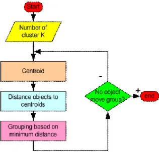
18 So, the main steps of K-Means algorithm are:
1. Select an initial partition with k clusters (repeat steps 2 and 3 until cluster membership stabilizes).
2. Generate a new partition by assigning each pattern to its closest cluster center. 3. Compute new cluster centers.
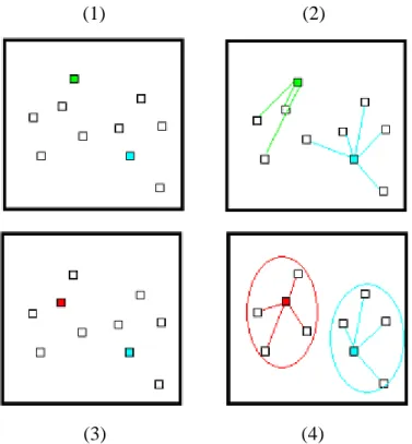
Figure 3.4 illustrates this process, as well Figure 3.5. Starting with two random points as centroids (1), the stage (2) assigns each point to the cluster nearest to it. In the stage (3), the associated points are averaged out to produce the new location of the centroid, leaving us with the final configuration (4). After each iteration the final configuration is fed back in to the same loop till the centroids converge.
(1) (2)
(3) (4)
19
Figure 3.5 – K-Means Algorithm Process
Table 3.2 presents some distance functions, including the Euclidean distance while Table 3.3 indicates the most common choices for proximity, centroids and objective functions specially for K-Means. The Eucliden distance is the distance metric that we are going to use in this study.
20
Proximity Function Centroid Objective Function
Manhattan median Minimize sum of the distance of an object to its cluster centroid
Squared Euclidean mean Minimize sum of the squared distance of an object to its cluster centroid
cosine mean Minimize sum of the cosine similarity of an object to its cluster centroid
Bregman divergence mean Minimize sum of the Bregman divergence of an object to its cluster centroid
Table 3.3 – K-Means: Common choices for proximity, centroids, and objective
functions (Adapted from Tan et al, 2006)
3.4.2. K-Medoids Clustering
Medoids is an extension of the basic Means algorithm (Jain, 2009). In K-Medoids, clusters are represented using the median of the data instead of the mean (Jain, 2009). Taking as reference point a medoid, which is the most centrally located object in a cluster (Velmurugan and Santhanam, 2010) this algorithm, compared to the K-Means, is less sensitive to outliers5 that produce very large distances. Despite the advantage of K-Medoids relatively to K-Means, K-Medoids is far more computationally intensive than K-Means (Hastie et al, 2001).
K-Medoids method can be, as well, performed based on the principle of minimizing the sum of the dissimilarities between each object and its corresponding reference point (Velmurugan and Santhanam, 2010).
According to Velmurugan and Santhanam (2010), the basic strategy of K-Medoids clustering algorithms is to find k clusters in n objects by first arbitrarily finding a representative object (the medoids) for each cluster. Each remaining object is clustered with the medoid to which it is the most similar. K-Medoids method uses representative objects as reference points. The algorithm takes the input parameter k, the number of clusters, to be partitioned among a set of n objects.
5
Outlier is an item whose value falls outside the bounds enclosing most of the other corresponding values in the sample. May indicate anomalous data, however should be examined carefully because may carry important information.
21
Velmurugan and Santhanam (2010) present a typical K-Medoids algorithm for partitioning based on medoid, as follows:
Input: K = number of clusters and D = dataset containing n objects
Output: A set of k clusters that minimizes the sum of the dissimilarities of all the objects to their nearest medoid.
Method: Arbitrarily choose k objects in D as the initial representative objects. Repeat: Assign each remaining object to the cluster with the nearest medoid; Randomly select a non medoid object Orandom; Compute the total points S of swap point Oj with Orandom; If S<0 then swap Oj with Orandom to form the new set of k medoid until no change.
Velmurugan and Santhanam (2010) compared the two algotrithms and concluded that “Means algorithm is more efficient for smaller datasets and K-Medoids algorithm seems to perform better for large datasets.”
3.5. Cluster Validity
After applying a clustering algorithm, we would like to know if the results reflect or not an innate property of the data (Mirkin, 2005). In other words, we want to know whether the cluster structure found is valid or not (Mirkin, 2005).
So, cluster validity refers to formal procedures that evaluate the results of cluster analysis in a quantitative and objective manner (Jain, 2009). Before a clustering algorithm is applied to the data, we should determine if data has, in fact, a clustering tendency6 (Jain, 2009).
In literature we can find several measures for cluster validation, including many cluster validity indices which can be defined based on three different criteria: internal, relative or external (Jain, 2009). Internal indices assess the fit between the structured imposed by the clustering algorithm (clustering) and the data using only the data. The better the indices value, the more reliable is the cluster structure Mirkin (2005). Relative indices compare multiple structures (generated by different algorithms, for example) and decide which of them is better in some sense. External indices measure the performance by matching cluster structure to the a priori information. Typically, clustering results are evaluated using the external criterion.
6
Mirkin (2005) defines cluster tendency as a description of a cluster in terms of the advantage values of relevant features.
22
Furthermore, according to Mirkin (2005), it is still possible to use another procedure for validating a cluster structure or clustering algorithm, it is called resampling. A resampling is used to see whether the cluster structure is stable when the data is changed. The cluster stability is measured as the amount of variation in the clustering solution over different subsamples drawn from the input data and different measures of that variation can be used to obtain different stability measures (Jain, 2009). For instance, in model based algorithms, as K-Means, the distance between the models found for different subsamples can be used to measure the stability.
In general, cluster validity indices are usually defined by combining compactness and separability. Compactness measures the closeness of cluster elements, being a common measure of that the variance. Separability indicates how distinct two clusters are being the distance between representative objects of two clusters a good example. This measure has been widely used due to its computational efficiency and effectiveness (Rendón et al, 2011).
The following tables describe some of the internal and external cluster validity indices most widely used and Figure 3.6 synthesizes the classification of the validation techniques.
Name Expression Description
Bayesian Information Criterion (BIC)
- Is devised to avoid overfitting. - n = number of objects
- L = the likelihood of parameters to generate the data in the model - v = number of free parameters in Gaussian model
- Takes into account both fit of the model to the data and the complexity of the model.
- A model that has a smaller BIC is better.
Calinski-Harabasz
- = the between-cluster scatter matrix
23
Name Expression Description
- = the number of clustered samples - k = the number of clusters
Davies-Bouldin (DB)
- Aim to identify sets of clusters that are compact and well separated. - c = the number of clusters - i, j = cluster labels
- d( ) and d( ) = all samples in clusters i and j to their respective cluster centroids
- d( ) = the distance between centroids
- Smaller value of DB indicates a better clustering solution.
Silhouette
For a given cluster, (j=1,…c), it assigns to the ith sample of a quality measure, s(i)= (i=1,…m), the silhouette width. This value is a confidence indicator of the membership of the ith sample in the cluster .
a = the average distance between the ith sample and all of samples included in
.
b(i) = the minimum average distance between the ith sample and all samples clustered in (k=1,…c; k ≠ j)
Dunn
- d( ) = the intercluster distance between cluster and
- d( ) = the intracluster distance of cluster ( )
- c = the number of cluster of dataset - Large values of index Dun correspond
24
Name Expression Description
to good clustering solution.
NIVA
- { } - (i=1,2,…,N)
-N = the number cluster from C
- Compac (C): average of compactness product (Esp( )) of c groups and separability between them (SepxS( ))
- SepxG (C): average separability of C groups
- The smaller value NIVA(C) indicates that avalid optimal partition to the different given partitions was found.
Table 3.4 – Internal Validity Indices (Adapted from Rendón et al, 2011)
Name Expression Description
F-Measure
- Combines the precision and recall concepts from information retrieval. Then calculate them of that cluster for each class.
- = the number of objects of class i that are in cluster j
- = the number of objects in cluster j
- = the number of objects in class i - The F-Measure values are within
25
Name Expression Description
the interval [0, 1] and larger values indicate higher clustering quality.
Nmimeasure
- NMI – Normalized Mutual Information
- I(X,Y) = the mutual information between two random variables X and Y
- H(X) = the entropy of X - X = consensus clustering - Y = the true labels
Purity
- We calculate the purity of a set of clusters. First, we cancel the purity in each cluster. For each cluster we have the purity
- = the number of objects in j with class label i
- = a fraction of the overall cluster size that the largest class of objects assigned to that cluster represents. - The overall purity of the clustering solution is obtained as a weighted sum of the individual cluster purities. - = the size of cluster j
- m = the number of clusters - n = the total number of objects
Entropy
- Measures the purity of the clusters class labels.
- If all clusters consist of objects with only a single class label, the entropy is 0.
- As the class labels of objects in a cluster become more varied, the
26
Name Expression Description
entropy increases.
- To compute the entropy of a
dataset, we need to calculate the class distribution of objects in each cluster
, where the sum is taken over all the classes.
- The total entropy for a set of clusters is calculated as the weighted sum of the entropies of all clusters. - = the size of cluster j
- m = the number of clusters
- n = the total number of data points
Table 3.5 – External Validity Indices (Adapted from Rendón et al, 2011)
Figure 3.6 – A Simplified Classification of Validation Techniques
27
4. SEGMENTATION IN MARKETING
“Do not buy market share. Figure out how to earn it.”
Philip Kotler in Marketing Management, 11th Edition
4.1. Segmentation Definition
Kotler (2005) defines market segmentation as “the act of dividing a market into smaller groups of buyers with distinct needs, characteristics, or behaviors who might require separate products and/or marketing mixes.” Despite that definition, there is another one that is considered the best by marketers given by Smith (1956): “market segmentation involves viewing a heterogeneous market as a number of smaller homogeneous markets, in response to differing preferences, attributable to the desires of consumers for more precise satisfaction of their varying wants.”
According to Wedel and Kamakura (2002), in market segmentation one distinguishes homogeneous groups of customers who can be targeted in the same manner because they have similar needs and preferences. For them, market segments are not real entities naturally occurring in the marketplace, but groupings created by managers to help them develop strategies that better meet consumer needs at the highest expected profit for the company. Therefore, segmentation is a very useful concept to managers.
4.2. Segmentation Effectiveness
According to Kotler (2000), an effective segmentation must meet some criteria. The segments must be measurable (the size, purchasing power, profiles of segments can be measure), substantial (segments must be large or profitable enough to serve), accessible (segments must be effectively reached and served), differentiable (segments must respond differently to different marketing mix elements and actions), and actionable (must be able to attract and serve the segments).
28
For Wedel and Kamakura (2000) the criteria that determine the effectiveness and profitability of marketing strategies are six and are described on Table 4.1.
Criteria Description
1 Identifiability
Is the extent to which managers can recognize distinct groups of customers in the marketplace by using specific segmentation bases. They should be able to identify the customers in each segment on the basis of variables that are easily measured.
2 Substantiality
This criterion is satisfied if the targeted segments represent a large enough portion of the market to ensure the profitability of targeted marketing programs. In the limit, this criterion may be applied to each individual customer.
3 Accessibility Is the degree to which managers are able to reach the targeted
segments through promotional or distributional efforts.
4 Responsiveness
This criterion is satisfied if the segments respond uniquely to marketing efforts targeted to them. It is critical because differentiated marketing mixes will be effective only if each segment is homogeneous and unique in its response to them.
5 Stability
It is necessary, at least for a period long enough for identification of the segments, implementation of the segmented marketing strategy, and the strategy to produce results. Only segments that are stable in time can provide the underlying basis for the development of a successful marketing strategy.
6 Actionability
This criterion is satisfied if the identification of the segments provides guidance for decisions on the effective specification of marketing instruments. The focus is on whether the customers in the segment and the marketing mix necessary to satisfy their needs are consistent with the goals and core competences of the company.
29
4.3. Segmentation Process
Marketers are increasingly combining several variables in an effort to identify smaller, better-defined target groups. This has led some market researchers to advocate a needs-based market segmentation approach (Kotler, 2008). Thus a seven-step segmentation approach was proposed by Best (2005), which steps are described on Table 4.2.
Steps Description
1 Needs-based Segmentation
Group customers into segments based on similar needs and benefits sought by customer in solving a particular consumption problem.
2 Segment Identification
For each needs-based segment, determine which demographics, lifestyles, and usage behaviors make the segment distinct and identifiable (actionable).
3 Segment Attractiveness
Using predetermined segment attractiveness criteria (such as market growth, competitive intensity, and market access) determine the overall attractiveness of each segment.
4 Segment
Profitability Determine segment profitability.
5 Segment Positioning
For each segment, create a “value proposition” and product-price positioning strategy based on that segment’s unique customer needs and characteristics.
6 Segment “Acid Test”
Create “segment storyboard” to test the attractiveness of each segment’s positioning strategy.
7 Marketing-Mix Strategy
Expand segment positioning strategy to include all aspects of the marketing-mix: product, price, promotion and place.
Table 4.2 – Steps in Segmentation Process
30
4.4. Levels of Market Segmentation
Because buyers have unique needs and wants, each buyer is potentially a separate market. Ideally, then, a seller might design a separate marketing program for each buyer. However, although some companies attempt to serve buyers individually, many others face larger numbers of smaller buyers and do not find complete segmentation worthwhile. Instead, they look for broader classes of buyers who differ in their product needs or buying responses. Thus, market segmentation can be carried out at several different levels (Kotler, 2008).
Figure 4.1 – Levels of Marketing Segmentation
Figure 4.1 shows that companies can practice no segmentation (mass marketing), complete segmentation (micromarketing), or something in between (segment marketing or niche marketing).
Levels of Marketing Segmentation
Mass Marketing Same product to all consumers No
Segmentation
Segment Marketing Different products to one or more
segments
Some
Segmentation
Niche Marketing Different products to subgroups within
segments
More
Segmentation
Micromarketing Products to suit the tastes of individuals or
locations
Complete Segmentation
Table 4.3 – Levels of Marketing Segmentation
Mass Marketing Segment Marketing Niche Marketing Micro Marketing
31
4.4.1. Mass Marketing
Companies have not always practiced target marketing. In fact, for most of the 1900s, major consumer products companies held fast to mass marketing—mass producing, mass distributing, and mass promoting about the same product in about the same way to all consumers. The traditional argument for mass marketing is that it creates the largest potential market, which leads to the lowest costs, which in turn can translate into either lower prices or higher margins. However, many factors now make mass marketing more difficult. The proliferation of distribution channels and advertising media has also made it difficult to practice "one-size-fits-all" marketing (Kotler, 2008).
4.4.2. Segment Marketing
A company that practices segment marketing isolates broad segments that make up a market and adapts its offers to more closely match the needs of one or more segments. Segment marketing offers several benefits over mass marketing. The company can market more efficiently, targeting its products or services, channels, and communications programs toward only consumers that it can serve best and most profitably. The company can also market more effectively by fine-tuning its products, prices, and programs to the needs of carefully defined segments. The company may face fewer competitors if fewer competitors are focused on this market segment (Kotler, 2008).
4.4.3. Niche Marketing
Market segments are normally large, identifiable groups within a market. Niche marketing focuses on subgroups within the segments. A niche is a more narrowly defined group, usually identified by dividing a segment into sub segments or by defining a group with a distinctive set of who may seek a special combination of benefits. Whereas segments are fairly large and normally attract several competitors, niches are smaller and normally attract only one or a few competitors. Niche marketers presumably understand their niches' needs so well that their customers willingly pay a price premium (Kotler, 2008).
32
4.4.4. Micro Marketing
Segment and niche marketers tailor their offers and marketing programs to meet the needs of various market segments. At the same time, however, they do not customize their offers to each individual customer. Thus, segment marketing and niche marketing fall between the extremes of mass marketing and micro marketing. Micro marketing is the practice of tailoring products and marketing programs to suit the tastes of specific individuals and locations. Micro marketing includes local marketing (involves tailoring brands and promotions to the needs and wants of local customer groups—cities, neighborhoods, and even specific stores) and individual marketing (tailoring products and marketing programs to the needs and preferences of individual customers) (Kotler, 2008).
4.5. Segmentation Bases
Wedel and Kamakura (2000) define segmentation basis as “a set of variables or characteristics used to assign potential customers to homogeneous groups.” They classify segmentation bases into four categories, which are presented in Table 4.4.
Bases
General Product-specificObservable
Cultural, geographic, demographic and socio-economic variables
User status, usage frequency, store loyalty and patronage, situations
Unobservable Psychographics, values,
personality and life-cycle
Psychographics, benefits, perceptions, elasticities, attributes, preferences, intention
Table 4.4 – Classification of Segmentation Bases
(Source: Wedel and Kamakura, 2000)
General segmentation bases are independent of products, services or circumstances and product-specific segmentation bases are related to customer and product, service and/or particular circumstances. Furthermore, observable segmentation bases are measured directly and unobservable segmentation bases are inferred.
33
4.5.1. Observable General Bases
In market segmentation, a widely number of bases are used in this category, such us cultural variables, geographic variables, neighborhood, geographic mobility, demographic and socio-economic variables, postal code classifications, household life cycle, household and company size, standard industrial classifications and socioeconomic variables. Also used are media usage and socioeconomic status (Wedel and Kamakura, 2000). The observable general bases play an important role in segmentation studies, whether simple or complex, and are used to enhance the accessibility of segments derived by other bases (Wedel and Kamakura, 2000).
4.5.2. Observable Product-Specific Bases
This kind of segmentation bases include variables that are related to buying and consumption behavior, like user status, usage frequency, brand loyalty, store loyalty, store patronage, stage of adoption and usage situation. These variables have been used both for consumer and business markets (Wedel and Kamakura, 2000).
4.5.3. Unobservable General Bases
Three groups of variables in this class of segmentation bases are identified: (1) personality traits, (2) personal values and (3) lifestyle.
The first may include dogmatism, consumerism, locus of control, religion and cognitive style. The most frequently used scale for measuring general aspects of personality in marketing is the Edward’s personal schedule.
Relatively to the second, the most important instrument to measure human values and to identify value systems is the Rokeach value survey.
The third is based on three components: activities (work, hobbies, social events, vacation, entertainment, clubs, community, shopping, sports), interests (family, home, job, community, recreation, fashion, food, media, achievements) and opinions (of oneself, social issues, politics, business, economics, education, products, future, culture).The lifestyle typology most used is the VALS system, which has been recently reviewed giving its place to the VALS2 system. It is defined by two main dimensions: resources (income, education, self-confidence, health, eagerness to buy, intelligence, etc.) and self-orientation (principle-oriented, self-oriented and status-oriented).These three groups of variables are used almost exclusively for consumer markets giving us “a
34
more lifelike picture of consumers and a better understanding of their motivations” (Wedel and Kamakura, 2000).
4.5.4. Unobservable Product-Specific Bases
This class of segmentation bases comprises product-specific psychographics, product-benefit perceptions and importance, brand attitudes, preferences and behavioral intentions. In these order, the variables form a hierarchy of effects, as each variable is influenced by those preceding it. Many of these variables are used for consumer markets; however they can also be used for segmenting business markets (Wedel and Kamakura, 2000).
All the segmentation bases are summarized on Table 4.5 according to the six criteria for effective segmentation.
Criteria
Bases
Id en tif iab il it y S u st ain n ab il it y Ac ce ss ib il it y S tab il it y Ac tion ab il it y Re sp on sivenes s General, Observable ++ ++ ++ ++ - - Specific, Observable - Purchase + ++ - + - + - Usage + ++ + + - + General, Unobservable - Personality +- - +- +- - - - Lifestyle +- - +- +- - - - Psycographics - +- +- - - Specific, Unobservable - Psycographics +- + - - ++ +- - Perceptions +- + - - + - - Benefits + + - + ++ ++ - Intentions + + - +- - ++++ very good, + good, +- moderate, - poor, -- very poor
Table 4.5 – Evaluation of Segmentation Bases