arXiv:1404.1071v1 [hep-ex] 3 Apr 2014
EUROPEAN ORGANISATION FOR NUCLEAR RESEARCH (CERN)
CERN-PH-EP-2014-034
Submitted to: Physical Review D
Measurement of the parity-violating asymmetry parameter
α
b
and the helicity amplitudes for the decay
Λ
0
b
→
J/ψΛ
0
with the
ATLAS detector
The ATLAS Collaboration
Abstract
A measurement of the parity-violating decay asymmetry parameter,
α
b, and the helicity amplitudes
for the decay
Λ
0b
→ J/ψ(µ
+µ
−)Λ
0(pπ
−)
is reported. The analysis is based on 1400
Λ
0band
Λ
¯
0bbaryons
selected in
4.6
fb
−1of proton–proton collision data with a center-of-mass energy of 7 TeV recorded
by the ATLAS experiment at the LHC. By combining the
Λ
0band
Λ
¯
0bsamples under the assumption of
CP
conservation, the value of
α
bis measured to be
0.30 ± 0.16(stat) ± 0.06(syst)
. This measurement
provides a test of theoretical models based on perturbative QCD or heavy-quark effective theory.
c
Measurement of the parity-violating asymmetry parameter
α
band the helicity
amplitudes for the decay Λ
0b
→
J/ψΛ
0
with the ATLAS detector
The ATLAS Collaboration
(Dated: April 4, 2014)
A measurement of the parity-violating decay asymmetry parameter, αb, and the helicity
ampli-tudes for the decay Λ0
b→ J/ψ(µ
+µ−)Λ0(pπ−) is reported. The analysis is based on 1400 Λ0 b and ¯Λ
0 b
baryons selected in 4.6 fb−1 of proton–proton collision data with a center-of-mass energy of 7 TeV
recorded by the ATLAS experiment at the LHC. By combining the Λ0
b and ¯Λ0b samples under the
assumption of CP conservation, the value of αb is measured to be 0.30 ± 0.16(stat) ± 0.06(syst).
This measurement provides a test of theoretical models based on perturbative QCD or heavy-quark effective theory.
PACS numbers: 14.20.Mr
I. INTRODUCTION
Parity violation, a well-known feature of weak inter-actions [1–4], is exhibited in its maximal form in decays of muons and τ leptons. However, in weak decays of hadrons, it is not maximal and depends on the hadron’s constituents because of the presence of strongly bound spectator quarks. For example, the process Λ0 → pπ−
has a parity-violating decay asymmetry parameter, αΛ,
of over 0.6 [5]. The decay asymmetry parameter α enters into the angular distribution of any two-body spin 1/2 particle decay as follows:
w(cos θ) = 1
2(1 + αP cos θ), (1) where P is the polarization of the particle and θ is de-fined as the angle between the polarization vector and the direction of the decay product in the particle’s rest frame. The strong interaction effects in the hadron de-cays are non-perturbative, which makes it very difficult to predict the value of α, at least for light hadrons such as Λ0. However, in the case of heavy baryons, such as
Λ0b, the energy release in the decay of the b-quark is large
enough that the use of the factorization theorem and per-turbative QCD (pQCD) seems justified to compute the effects of the strongly coupled spectator quarks, making theoretical predictions possible.
Several models have been employed to predict the value of the parity-violating decay asymmetry parameter αb
for the weak decay Λ0
b → J/ψΛ0. Various quark models
are used to calculate the form factors in the factorization approximation (FA) [6–10] and the predictions of αb
gen-erally lie in the range from −0.2 to −0.1. In Ref. [11], the Λ0b → J/ψ(µ+µ−)Λ0(pπ−) decay process is factorized
into parts calculable in pQCD and universal hadron dis-tribution amplitudes, so both the factorizable and non-factorizable contributions in the FA are included. The value of αb is predicted to be in the range from −0.17
to −0.14. However, a calculation based on heavy-quark effective theory (HQET) [12,13] predicts a value 0.78.
Recently, the LHCb experiment reported a measure-ment of αb = 0.05 ± 0.17(stat) ± 0.07(syst) [14]. This
paper provides a measurement of comparable precision
using 4.6 fb−1 pp collision data recorded by the ATLAS
detector with a center-of-mass energy of 7 TeV.
II. THE Λ0
b→J/ψ(µ+µ−)Λ0(pπ−) DECAY
Because of parity conservation, Λ0
b produced by the
strong interaction, which is the dominant production mechanism, can be polarized only in a direction perpen-dicular to the Λ0
b production plane, ˆn [13,15]. The vector
ˆ
n is chosen to point in the direction of the cross product of the beam direction and the Λ0
b momentum. Since the
LHC collides proton beams traveling in opposite direc-tions, either beam direction could be used. This analysis uses the positive z-axis direction of the ATLAS coordi-nate system [16] for the Λ0
b candidates and the negative
z-axis for ¯Λ0
b candidates (to preserve symmetry between
Λ0 and ¯Λ0 given by the orientation of the ATLAS
mag-netic field). The definition of the decay angles is shown in Fig.1. The angle θ is the polar angle of the Λ0
mo-mentum measured from the normal direction ˆn in the Λ0 b
rest frame. The corresponding azimuthal angle, φ, is of no interest in this analysis and therefore is not labeled in the figure. The angles θ1 (θ2) and φ1 (φ2) are the polar
and azimuthal angles of the proton (µ+) in the Λ0(J/ψ)
rest frame with respect to the Λ0 (J/ψ) direction in the
Λ0
b rest frame. The azimuthal angles, φ1 and φ2, are
measured in the right-handed coordinate systems of the rest frames of Λ0 and J/ψ, (x
1, y1, z1) and (x2, y2, z2),
respectively. The z1,2-axes are aligned with the direction
of Λ0 and J/ψ, respectively, and the x
1,2-axes lie in the
plane containing ˆn and the Λ0 or J/ψ momenta. With
this definition, the sum φ1+ φ2 gives the angle between
the Λ0and J/ψ decay planes.
Taking λΛ and λJ/ψ to represent the helicity of the Λ0
and the J/ψ, the decay Λ0
b → J/ψΛ0 can be described
by four helicity amplitudes A(λΛ, λJ/ψ): a+≡ A(1/2, 0),
a− ≡ A(−1/2, 0), b+≡ A(−1/2, −1) and b−≡ A(1/2, 1),
which are normalized to unity:
|a+|2+ |a−|2+ |b+|2+ |b−|2= 1. (2)
FIG. 1. The decay angles, as defined in the text.
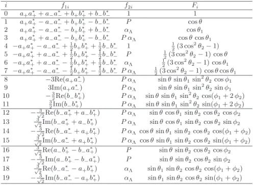
the decay angles Ω = (θ, φ, θ1, φ1, θ2, φ2) is [15,17,18]:
w(Ω, ~A, P ) = 1 (4π)3 19 X i=0 f1i( ~A)f2i(P, αΛ)Fi(Ω), (3)
with the 20 terms f1i, f2i and Fi listed in Table I. ~A
represents the four helicity amplitudes and P is the po-larization of Λ0
b. Under the assumption of CP
conserva-tion in Λ0 → pπ− and ¯Λ0 → ¯pπ+ decays, α ¯
Λ = −αΛ =
−0.642 ± 0.013 is used in this analysis, because the value αΛ = 0.642 ± 0.013 is measured with better precision
than its counterpart αΛ¯ = −0.71 ± 0.08 [19]. The Fi(Ω)
are orthogonal functions of the decay angles.
The αb parameter is related to the helicity amplitudes
as follows [15]:
αb= |a+|2− |a−| 2+ |b
+|2− |b−|
2. (4)
There are nine unknown real parameters in the PDF (Eq. (3)): four complex helicity amplitudes, a+ =
|a+|eiρ+, a− = |a−|eiρ−, b+ = |b+|eiω+, b
− = |b−|eiω−, each with a magnitude and a phase, and the polarization P . However, only six out of the eight helicity amplitude parameters are independent, taking into account the nor-malization constraint (Eq. (2)) and, due to the arbitrary value of the common phase, only differences between the four phases are relevant.
The angular PDF is further simplified due to the sym-metry of the initial state at a pp collider. Since the arbitrary choice of the beam direction cannot bear on the physics result, the polarization must be an odd func-tion of the Λ0
b pseudorapidity: P (pT, η) = −P (pT, −η).
Therefore, for a sample of Λ0
b produced over a symmetric
interval in pseudorapidity, which is satisfied in the AT-LAS detector, the average polarization must be zero. As a result, only six terms in TableI which are not depen-dent on P are retained in the PDF and they depend only
on five independent parameters: three magnitudes of the helicity amplitudes and two relative phases. The remain-ing phase cannot be resolved with a zero-polarization sample, but αb can be determined from the magnitudes
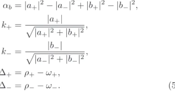
of the helicity amplitudes as in Eq. (4). The following choice of the fit model parameterization is found to have only a small correlation of uncertainties and is used in this analysis: αb= |a+|2− |a−| 2+ |b +|2− |b−| 2, k+= |a+| p|a+|2+ |b+|2 , k−= |b−| p|a−|2+ |b −|2 , ∆+= ρ+− ω+, ∆−= ρ−− ω−. (5)
Table II shows the explicit dependence of the f1i
func-tions on the chosen parameters.
If CP is conserved, the PDFs of the Λ0
b and ¯Λ0b decays
have exactly the same form. Therefore, assuming CP conservation, the Λ0b and ¯Λ0b samples are combined to
measure αb and the helicity amplitudes.
III. DATA SAMPLES AND TRIGGER
SELECTION
ATLAS [20] covers nearly the entire solid angle around the interaction point with layers of tracking detectors, calorimeters, and muon chambers. This analysis uses two sub-systems: the inner detector (ID) and the muon spectrometer (MS). The ID consists of three types of de-tectors: a silicon pixel detector (Pixel), a silicon micro-strip detector (SCT) and a transition radiation tracker (TRT). These detectors are surrounded by a thin su-perconducting solenoid providing a 2 T axial magnetic field. The MS measures the deflection of muons in a magnetic field produced by three large superconducting air-core toroid systems, each with eight superconducting coils, and it consists of four sub-detectors. Monitored drift tube chambers and cathode strip chambers are used for precision muon measurements, while resistive plate chambers (RPCs) and thin gap chambers (TGCs) are used by the muon trigger system. The MS and ID pro-vide a pseudorapidity coverage up to |η| = 2.5. Tracks reconstructed in the ID with pT> 400 MeV are used in
this analysis.
This analysis uses 7 TeV collision data collected in 2011 with single-muon triggers and the dimuon triggers used to select J/ψ → µ+µ−. The corresponding integrated
luminosity is 4.6 fb−1 [21]. The ATLAS trigger system
[22] has three levels: the hardware-based Level-1 trigger and the two-stage High-Level Trigger (HLT). At Level-1, the muon trigger uses RPCs and TGCs to search for patterns of hits corresponding to muons passing different pT thresholds. Regions of interest around these Level-1
TABLE I. The coefficients f1i, f2i and Fiof the probability density function in Eq. (3) [15]. i f1i f2i Fi 0 a+a∗++ a−a∗−+ b+b∗++ b−b∗− 1 1 1 a+a∗+− a−a∗−+ b+b∗+− b−b∗− P cos θ 2 a+a∗+− a−a∗−− b+b∗++ b−b∗− αΛ cos θ1 3 a+a∗++ a−a∗−− b+b∗+− b−b∗− P αΛ cos θ cos θ1 4 −a+a∗+− a−a∗−+ 1 2b+b∗++12b−b∗− 1 1 2(3 cos 2θ 2− 1)
5 −a+a∗++ a−a∗−+12b+b+∗ −12b−b−∗ P 12(3 cos2θ2− 1) cos θ
6 −a+a∗++ a−a∗−− 1 2b+b∗++12b−b∗− αΛ 12(3 cos 2θ 2− 1) cos θ1 7 −a+a∗+− a−a∗−− 1 2b+b∗+−12b−b∗− P αΛ 12(3 cos 2θ 2− 1) cos θ cos θ1
8 −3Re(a+a∗−) P αΛ sin θ sin θ1 sin
2
θ2 cos φ1
9 3Im(a+a∗−) P αΛ sin θ sin θ1 sin2θ2sin φ1
10 −3
2Re(b−b∗+) P αΛ sin θ sin θ1sin2θ2 cos(φ1+ 2 φ2)
11 3
2Im(b−b∗+) P αΛ sin θ sin θ1 sin2θ2 sin(φ1+ 2 φ2)
12 − 3
√
2Re(b−a∗++ a−b∗+) P αΛ sin θ cos θ1 sin θ2cos θ2 cos φ2
13 3
√
2Im(b−a∗++ a−b∗+) P αΛ sin θ cos θ1 sin θ2 cos θ2 sin φ2
14 − 3
√
2Re(b−a∗−+ a+b∗+) P αΛ cos θ sin θ1 sin θ2cos θ2 cos(φ1+ φ2)
15 3
√
2Im(b−a∗−+ a+b∗+) P αΛ cos θ sin θ1 sin θ2 cos θ2 sin(φ1+ φ2)
16 3
√
2Re(a−b∗+− b−a∗+) P sin θ sin θ2 cos θ2cos φ2
17 − 3
√
2Im(a−b∗+− b−a∗+) P sin θ sin θ2 cos θ2 sin φ2
18 3
√
2Re(b−a∗−− a+b∗+) αΛ sin θ1 sin θ2cos θ2cos(φ1+ φ2)
19 − 3
√
2Im(b−a∗−− a+b∗+) αΛ sin θ1 sin θ2 cos θ2 sin(φ1+ φ2)
TABLE II. The coefficients f1iof the remaining six terms of the simplified PDF expressed using the five free parameters defined
in Eq. (5). i f1i 0 1 2 (k2 ++ k−2 − 1) + αb(k2+− k−2) 4 1 4[(3k 2 −− 3k 2 +− 1) + 3αb(1 − k2 −− k 2 +)] 6 −1 4[(k 2 ++ k2−− 1) + αb(3 + k 2 +− k2−)] 18 3 √ 2[ 1−αb 2 q k2 −(1 − k 2 −) cos(−∆−) − 1+αb 2 q k2 +(1 − k2+) cos(∆+)] 19 − 3 √ 2[ 1−αb 2 q k2 −(1 − k 2 −) sin(−∆−) − 1+αb 2 q k2 +(1 − k+2) sin(∆+)]
hit patterns then serve as seeds for the HLT muon re-construction. When the rate from the low-pTmuon
trig-gers exceeded the allotted trigger bandwidth, prescale factors were applied to reduce the output rate. The transverse momentum threshold for unprescaled single-muon triggers was 18 GeV. The J/ψ → µ+µ− triggers
are dimuon triggers that require the muons to have op-posite charge and the dimuon mass to be in the interval 2.5 < mµµ< 4.3 GeV. Most of the sample was collected
by the J/ψ → µ+µ−trigger with a p
Tthreshold of 4 GeV
applied to both muons. This is the lowest pT threshold
trigger unprescaled in the 2011 data-taking period.
IV. MONTE CARLO SAMPLES
A Monte Carlo (MC) sample of signal events is used to study the efficiency and acceptance of the detector. In-clusive inelastic events are generated using the Pythia 6.4 MC generator [23] and filtered such that each event contains a signal decay, Λ0
b → J/ψ(µ+µ−)Λ0, with the
muons having transverse momenta above 2.5 GeV. In ad-dition to the Λ0
b MC sample, Bd0 → J/ψ(µ+µ−)KS0 and
b¯b → J/ψ(µ+µ−) + X MC samples are also generated
with the same generator-level muon cuts in order to op-timize the selection cuts and understand the sources of background. The MC events are passed through the AT-LAS simulation and reconstruction software [24] based on the Geant 4 [25] package for the detector simulation. The MC simulation and reconstruction software is con-figured to reproduce the detector conditions during data taking.
V. RECONSTRUCTION AND SIGNAL
SELECTION A. Muon Reconstruction
Two types of muons are used in the analysis, known as tagged muons and combined muons [26]. A charged-particle track reconstructed in the MS is matched to one
reconstructed in the ID to form a combined muon. The pseudorapidity coverage of combined muons is |η| < 2.5. Tagged muons, consisting of tracks reconstructed in the ID and matched to patterns of hits in the MS, cover the pseudorapidity range |η| < 2.2 and contribute to the muon reconstruction efficiency in the low-pT range.
Although both the ID and the MS provide a momen-tum measurement separately, only the ID measurement is used because of its better resolution in the pT range
relevant for this analysis, and the MS is used only to iden-tify muons. The reconstructed muon tracks are required to have a sufficient number of hits in the Pixel, SCT and TRT detectors to ensure accurate ID measurements.
B. J/ψ and Λ0 Preselection
The decay Λ0b → J/ψ(µ+µ−)Λ0(pπ−) has a cascade
topology, as the J/ψ decays instantly at the same point as the Λ0
b (forming a secondary vertex) while Λ0 lives
long enough to form a displaced tertiary vertex.
The J/ψ candidates are selected by fitting dimuon pairs to a common vertex [27] and requiring that their invariant mass lies in the range 2.8 < mµµ < 3.4 GeV.
The dihadron pairs are also fitted to a common vertex and accepted as Λ0 candidates if the invariant mass is
in the range 1.08 < mpπ < 1.15 GeV. The tracks used
for the primary vertex reconstruction are excluded from the Λ0 vertex fit to reduce the large combinatorial
back-ground. The masses of a proton and a pion are assigned to the tracks when the invariant mass is calculated; pπ−
and ¯pπ+ combinations are considered so that both the
Λ0 and ¯Λ0candidates are accepted.
C. Reconstruction of Λ0
b→J/ψ(µ+µ−)Λ0(pπ−)
The preselected muon and hadron track pairs are then refitted with a constraint to the Λ0
b →
J/ψ(µ+µ−)Λ0(pπ−) topology. The muons are required
to intersect at a single vertex and their invariant mass is constrained to the mass of the J/ψ, mJ/ψ =
3096.9 MeV [19]. The two hadron tracks are forced to intersect in a second vertex and their invariant mass is fixed to the mass of the Λ0, m
Λ0 = 1115.7 MeV [19]. The combined momentum direction of the refitted Λ0
track pair is constrained to point to the dimuon vertex. Two mass hypotheses are considered: the first assigns the proton mass to the positive track and the pion mass to the negative track, and the second hypothesis makes the opposite mass assignment. These hypotheses correspond to Λ0
b and ¯Λ0b decays, respectively. The fit is performed
on all four tracks simultaneously, taking into account the constraints described above [27]. The quality of the fit is characterized by the value of χ2 divided by the number of degree of freedom, Ndof. Furthermore, for each track
quadruplet that can be successfully fitted to the Λ0 bdecay
topology, a fit to the B0
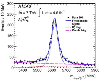
d→ J/ψ(µ+µ−)KS0(π+π−) decay [MeV] ) 0 Λ ( 0 Λ ψ J/ m 5400 5500 5600 5700 5800 5900 Events / 10 MeV 0 50 100 150 200 250 300 Data 2011 Fitted model Signal bkg d 0 B Comb. bkg ATLAS -1 L dt = 4.6 fb
∫
= 7 TeV, s 0 b Λ + 0 b ΛFIG. 2. The reconstructed mass of Λ0
b and ¯Λ0b candidates,
fitted with a three-component PDF (blue solid curve) con-sisting of signal (blue dashed curve), combinatorial (magenta long-dashed straight line) and B0
dbackground (red dot-dashed
curve, bottom).
topology is attempted (i.e. the pion mass is assigned to the hadron tracks and the dihadron mass is constrained to the mass of K0
S, mKS = 497.6 MeV [19]). The B 0 d fit
is needed to identify possible B0
d decays misidentified as
Λ0 b.
The fitted Λ0
b are further required to pass following
selection cuts (see Ref. [28] for details): • The fit quality χ2/N
dof < 3.
• The transverse momentum of the refitted Λ0,
pT,Λ0> 3.5 GeV.
• The transverse decay length of the refitted Λ0
ver-tex measured from the Λ0
b vertex, Lxy,Λ0> 10 mm. • If the four tracks forming a Λ0
b candidate also result
in an acceptable B0
d fit, the candidate must have
a larger cumulative χ2 probability for the Λ0b fit:
PΛ0 b > PB
0 d.
• The reconstructed Λ0
b proper decay time [28], τ >
0.35 ps.
Figure 2 shows the invariant mass distribution of events passing these selection cuts in the range from 5340 MeV to 5900 MeV. There is no track quadruplet simultaneously satisfying both the Λ0
b and ¯Λ0b
hypothe-ses. Background events can be divided into two cate-gories: the combinatorial background and the peaking background. The combinatorial background consists of real or fake J/ψ and Λ0 candidates randomly combined to create a Λ0
b-like topology. This is the main
com-ponent of the background, whose mass distribution is non-resonant and assumed to be linear in the vicinity of
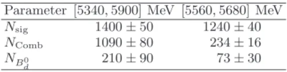
TABLE III. The numbers of signal candidates, Nsig,
combi-natorial background, NComb, and Bd0 background candidates,
NB0
d, extracted by the extended binned maximum likelihood fit in the mass range from 5340 MeV to 5900 MeV. The num-ber of events from each component in the SR mass window is given by scaling the values from the fit.
Parameter [5340, 5900] MeV [5560, 5680] MeV
Nsig 1400 ± 50 1240 ± 40
NComb 1090 ± 80 234 ± 16
NB0
d 210 ± 90 73 ± 30
the Λ0
b mass. The peaking background is due to
resid-ual Bd0→ J/ψ(µ+µ−)KS0(π+π−) decays passing the
re-quirement PΛ0 b > PB
0
d. The invariant mass distribu-tion is fitted with a three-component PDF to estimate the number of signal, combinatorial background and B0 d
background events. The shapes of the Λ0
b signal
com-ponent and the B0
d background are modeled using
one-dimensional Gaussian-kernel estimation PDFs [29] of the MC events. The Gaussian-kernel estimators are non-parametric PDFs describing the shape of the invariant mass distribution of the MC candidates (i.e. MC tem-plates). The advantage of using MC templates is that they accurately describe the non-Gaussian tails of the Λ0
b peak as well as the asymmetry of the Bd0background,
which is important in correctly estimating the number of events in the fit. The effect of possible mis-modeling of the shape of mJ/ψΛ0in the signal MC sample is discussed in Sec. VII. The combinatorial background is parame-terized by a first-order polynomial. An extended binned maximum likelihood fit [30] is performed with the number of events corresponding to each PDF component (Nsig,
NComb, and NB0
d) and the slope of the linear background PDF as free parameters.
The numbers of events extracted by the invariant mass fit are summarized in TableIII. A mass window around the nominal Λ0
b mass [19], 5560 < mJ/ψΛ0 < 5680 MeV, is defined as the signal region (SR) for this measurement. In the SR, the number of B0d events is nearly one fourth
of the total number of background events, and it has a large relative uncertainty due to its small size and the broad distribution of the B0
d peak.
VI. PARAMETER EXTRACTION
A. Least squares fit
The average values of the angular distributions Fi(Ω)
defined in TableI: hFii = 1 Ndata Ndata X n=1 Fi(Ωn) (6)
are used to extract the helicity parameters. By definition, hF0i is identical to one.
The expected values of hFii depend on the helicity
pa-rameters ~A and can be obtained by convolving these func-tions with the PDF (Eq. (3)) and integrating over the full angular range: hFiiexpected= X j f1i( ~A)f2i(αΛ)Cij, (7) with Cij = 1 (4π)3 Z Z Fi(Ω′)T (Ω′, Ω)Fj(Ω) dΩ′dΩ, (8)
where Ω stands for the true decay angles and Ω′ for the
measured ones. The acceptance, efficiency and resolution of the detector are represented by T (Ω′, Ω). These
detec-tor effects are encoded in the matrix C, whose elements do not depend on the helicity parameters, ~A.
Ideally, the helicity amplitude parameters can be cal-culated by solving the system of five equations with five parameters:
hFiiexpected= hFii, for i = 2, 4, 6, 18, and 19. (9)
However, with the measured values of hFii in current
data, Eq. (9) has no solution with real parameters. Therefore, the set of real parameters that are statisti-cally closest to the exact solution is found by minimizing the χ2function with respect to the five real parameters:
χ2=X
i
X
j
(hFiiexpected− hFii)Vij−1(hFjiexpected− hFji),
(10) where i, j = 2, 4, 6, 18 and 19, and V is the covariance matrix of the measured hFii values. The correlations
between the five averages are accounted for by the co-variance matrix.
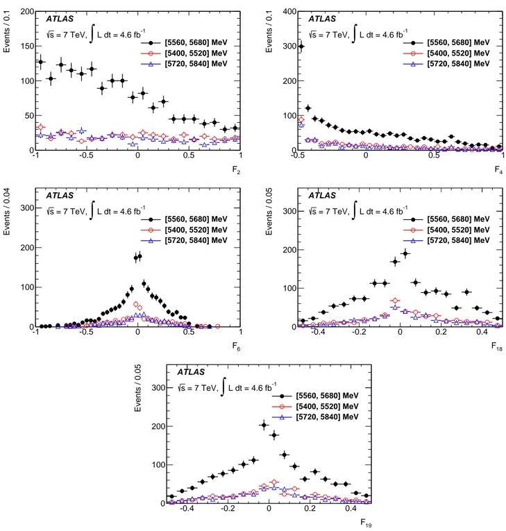
B. Background subtraction
As the combinatorial background can be described by the linear function, its contribution to the measured hFii
values can be estimated by using events in the invariant mass sidebands. Two mass windows define the sidebands: 5400 < mJ/ψΛ0 < 5520 MeV is chosen as the left side-band and 5720 < mJ/ψΛ0 < 5840 MeV as the right one. The background contribution to the hFii values in the
signal region is estimated as an average of the values in the two sidebands and is subtracted from the measured value of hFii.
The similarity of the left and right sidebands can be verified by comparing the Fi distributions. Figure 3
shows that the distributions for Fi are similar in the two
sidebands while the distributions in the signal region are different. The only significant difference between the oc-cupancy of the two sidebands is when the value of F6 is
close to zero and is due to B0
d background.
The B0dMC sample, together with the estimated
num-ber of B0
d events (Sec.V C), is used to calculate the
con-tribution of the B0
d events to the averaged hFii values
2 F -1 -0.5 0 0.5 1 Events / 0.1 0 50 100 150 200 [5560, 5680] MeV [5400, 5520] MeV [5720, 5840] MeV ATLAS -1 L dt = 4.6 fb
∫
= 7 TeV, s 4 F -0.5 0 0.5 1 Events / 0.1 0 100 200 300 400 [5560, 5680] MeV [5400, 5520] MeV [5720, 5840] MeV ATLAS -1 L dt = 4.6 fb∫
= 7 TeV, s 6 F -1 -0.5 0 0.5 1 Events / 0.04 0 100 200 300 [5560, 5680] MeV [5400, 5520] MeV [5720, 5840] MeV ATLAS -1 L dt = 4.6 fb∫
= 7 TeV, s 18 F -0.4 -0.2 0 0.2 0.4 Events / 0.05 0 100 200 300 [5560, 5680] MeV [5400, 5520] MeV [5720, 5840] MeV ATLAS -1 L dt = 4.6 fb∫
= 7 TeV, s 19 F -0.4 -0.2 0 0.2 0.4 Events / 0.05 0 100 200 300 [5560, 5680] MeV [5400, 5520] MeV [5720, 5840] MeV ATLAS -1 L dt = 4.6 fb∫
= 7 TeV, sFIG. 3. The Fi (i = 2, 4, 6, 18, 19) distribution for events in the sidebands, together with the distribution for events in the
signal region.
C. Detector effects correction
In the case of an ideal detector, there are no acceptance and resolution effects, i.e. T (Ω′, Ω) = δ(Ω′, Ω), where
δ(Ω′, Ω) is the Dirac delta function. In this case, C is a
simple diagonal matrix D with elements Dij=
1 (4π)3
Z
Fi(Ω)Fj(Ω) dΩ. (11)
D= diag{1, 1/3, 1/5, 1/15, 2/45, 2/45} is diagonal due to the orthogonality of the terms Fi(Ω).
The T (Ω′, Ω) is subject to the detector effects (the
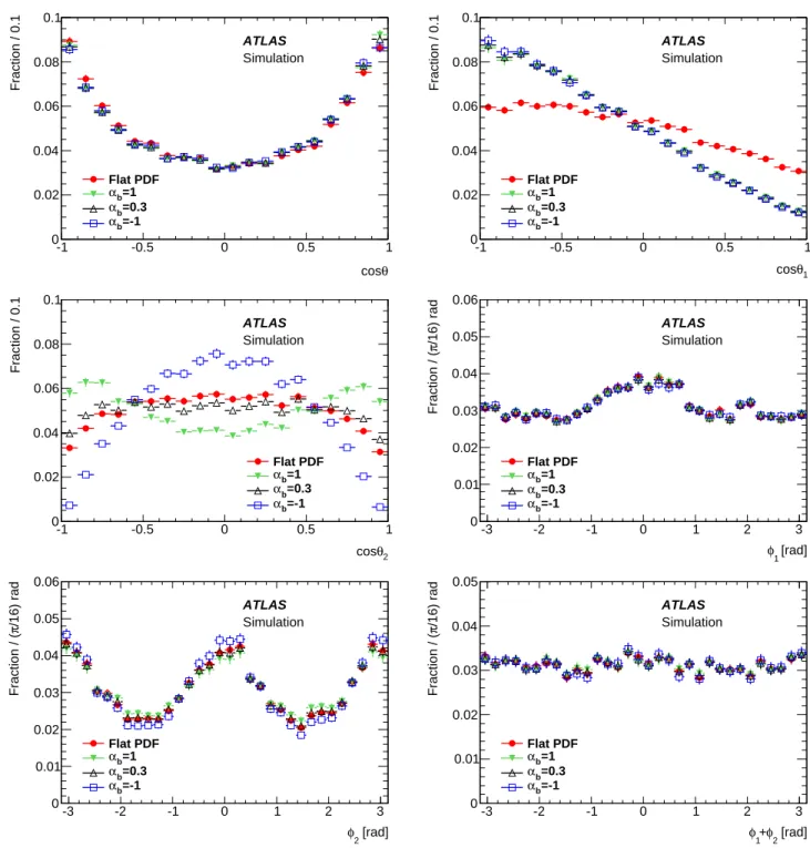
lim-ited acceptance of the detector, the detection and recon-struction efficiencies, and the resolution of the angular variables) that could affect the measured average of Fi.
Figure4shows the detector effects in the distribution of some angular variables for the MC events. At the level of MC generator level, without any simulation of the
detec-tor effects, the shown variables are uniformly distributed. Therefore, any structure observed in the distributions is due to detector effects. To illustrate the sensitivity, ad-ditional distributions in this figure show the same MC events re-weighted by three different PDFs with the val-ues of the parameters as given in the figure caption.
As shown in the preceding section, the matrix C is independent of the helicity amplitude parameters and can therefore be estimated using MC simulation, pro-vided the detector is correctly described. For every recon-structed MC event, values of the true and reconrecon-structed decay angles, Ω and Ω′, are known. Their PDF can be
written as
wmc(Ω′, Ω) = 1
ǫT
T (Ω′, Ω)wgen(Ω), (12)
where wgen(Ω) is the generator-level PDF and ǫ T is
the overall normalization factor. Since a uniform an-gular distribution is used to generate the MC sample, wgen(Ω) = 1, the distribution of angles Ω′ and Ω for the
reconstructed events is given solely by the detector ef-fects. Therefore, the function T (Ω′, Ω) is also the PDF
for the reconstructed MC events (except for the overall normalization factor ǫT), and Eq. (8) becomes a
calcula-tion of the mean of the expression Fi(Ω′)Fj(Ω) for
vari-ables Ω′ and Ω distributed according to T (Ω′, Ω). The
MC integration method is used to estimate the value of the coefficients Cij by replacing the integral with a
sum-mation: Cij= 1 (4π)3 Z Z Fi(Ω′)Fj(Ω)T (Ω′, Ω) dΩ′dΩ = ǫT (4π)3 Z Z Fi(Ω′)Fj(Ω) wmc(Ω′, Ω) dΩ′dΩ ≈ ǫT Nmc Nmc X n Fi(Ω′n)Fj(Ωn). (13)
The unknown normalization factor, ǫT, can be
deter-mined from the constraint hF0iexpected ≡ 1. The MC
events used in the matrix C calculation are required to satisfy the same selection criteria as data. In order to have the same kinematics as data, two types of weights are applied to the MC events. The first type is used to reproduce the same trigger configuration. The second one is used to reproduce the measured (pT, η)
distribu-tion of Λ0
b candidates. The latter weight is called the
kinematic weight and it is derived by comparing the two-dimensional 15 × 10 binned (pT, η) distribution of Λ0b in
MC simulation and sideband-subtracted data.
The matrix C used in this analysis after weighting is:
1 −0.113 −0.033 0.0074 0.0223 −0.0028 −0.112 0.3091 0.0071 −0.0133 0.0029 −0.0010 −0.033 0.0074 0.1775 −0.0186 0.0041 −0.0001 0.0071 −0.0133 −0.0185 0.0545 0.00013 0.00029 0.0221 0.0026 0.0040 0.00015 0.0465 0.0005 −0.0031 −0.0008 −0.0003 0.00034 0.0005 0.0450 . (14)
The MC statistical uncertainty of the elements on the di-agonal is about 1%, while the relative uncertainty of some
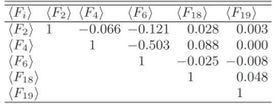
TABLE IV. Correlation matrix of the hFii measurements.
hFii hF2i hF4i hF6i hF18i hF19i hF2i 1 −0.066 −0.121 0.028 0.003 hF4i 1 −0.503 0.088 0.000 hF6i 1 −0.025 −0.008 hF18i 1 0.048 hF19i 1
of the off-diagonal elements is larger due to their small value. The impact of these uncertainties is discussed in Sec.VII.
D. Fit results
The measured values of the averages hFii after the
side-band subtraction and B0
d background correction are
hF2i = −0.282 ± 0.021,
hF4i = −0.044 ± 0.017,
hF6i = 0.001 ± 0.010,
hF18i = 0.019 ± 0.009,
hF19i = −0.002 ± 0.009. (15)
The correlations between these measurements are listed in TableIV. In general, the correlations are small, except for the correlation of hF4i and hF6i.
The χ2 fit (Eq. (10)) is applied to data and yields:
αb= 0.30 ± 0.16,
k+= 0.21+0.14−0.21,
k− = 0.13+0.20−0.13. (16)
The statistical uncertainty of the parameters are calcu-lated by finding the range that satisfies χ2− χ2
min < 1.
Negative values of k+ and k− are allowed but they will
give identical χ2, because the real values used in fit are
|k+| and |k−|. Thus, negative-value parts of their
un-certainty bands are truncated. With the limited data sample size, values of the relative phases, ∆+ and ∆−,
obtained from the fit, are consistent with the entire al-lowed range, [−π, π]. The effect of their large uncertain-ties on the determination of αb, k+ and k− is checked
in an alternative fit. Since the phase parameters are not well determined, and the efficiency of the measurement does not have a strong dependence on φ1+ φ2as shown
in Fig.4, only the first four terms in TableIIare consid-ered in the alternative fit and only the parameters αb, k+
and k− are determined. The results of this fit, both the
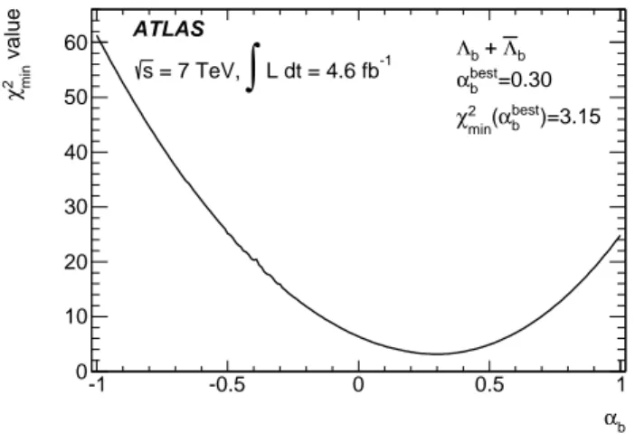
central values and the statistical uncertainties, are very similar to those of the main analysis. In particular, the differences between the central values are smaller than the statistical errors and comparable to the systematic uncertainties discussed in Sec. VII. Figure 5 shows the χ2
minas a function of the assumed αbparameter with the
θ cos -1 -0.5 0 0.5 1 Fraction / 0.1 0 0.02 0.04 0.06 0.08 0.1 Flat PDF =1 b α =0.3 b α =-1 b α ATLAS Simulation 1 θ cos -1 -0.5 0 0.5 1 Fraction / 0.1 0 0.02 0.04 0.06 0.08 0.1 Flat PDF =1 b α =0.3 b α =-1 b α ATLAS Simulation 2 θ cos -1 -0.5 0 0.5 1 Fraction / 0.1 0 0.02 0.04 0.06 0.08 0.1 Flat PDF =1 b α =0.3 b α =-1 b α ATLAS Simulation [rad] 1 φ -3 -2 -1 0 1 2 3 /16) rad π Fraction / ( 0 0.01 0.02 0.03 0.04 0.05 0.06 Flat PDF =1 b α =0.3 b α =-1 b α ATLAS Simulation [rad] 2 φ -3 -2 -1 0 1 2 3 /16) rad π Fraction / ( 0 0.01 0.02 0.03 0.04 0.05 0.06 Flat PDF =1 b α =0.3 b α =-1 b α ATLAS Simulation [rad] 2 φ + 1 φ -3 -2 -1 0 1 2 3 /16) rad π Fraction / ( 0 0.01 0.02 0.03 0.04 0.05 Flat PDF =1 b α =0.3 b α =-1 b α ATLAS Simulation
FIG. 4. Event distribution for each angular variable in simulated data after acceptance, efficiency and resolution effects are taken into account. The red filled points show the distributions in the default MC sample, where the generated distributions are uniform in all angular variables. For illustration of the sensitivity, the default MC events weighted using PDFs with αb= ±1
(green filled down triangles and blue open squares) and the measured value αb= 0.3 (open up triangles) are also shown. Other
parameters are set to k+= 0.21 and k−= 0.13 (measured values), and ∆+= ∆−= 0.
minimum of this conditional χ2
min curve gives the
cen-tral value of αb (αbestb ) and the corresponding χ2 value
is 3.15. The correlation matrix of the fitted parameters is shown in Table V. There are no strong correlations between these parameters. The corresponding absolute
values of the helicity amplitudes are |a+| = 0.17+0.12−0.17, |a−| = 0.59 +0.06 −0.07, |b+| = 0.79+0.04−0.05, |b−| = 0.08+0.13−0.08. (17)
b α -1 -0.5 0 0.5 1 value min 2 χ 0 10 20 30 40 50 60 b Λ + b Λ =0.30 best b α )=3.15 best b α ( min 2 χ ATLAS -1 L dt = 4.6 fb
∫
= 7 TeV, sFIG. 5. The conditional χ2
min as a function of αb.
TABLE V. Correlation matrix of the fitted parameters. Parameter αb k+ k−
αb 1 0.41 −0.19
k+ 1 0.20
k− 1
To check the fit results, the MC events are further weighted using the signal PDF with parameters deter-mined from the fit and normalized to the number of events of the sideband-subtracted data. These weighted MC events and sideband background distributions of Fi
are added and compared with data. Figure6shows good agreement between the weighted MC events and data.
The polarization of Λ0
b and ¯Λ0b is checked with data
and is found consistent with the expected value of zero (Sec. II). The combination of Λ0
b and ¯Λ0b samples is also
justified by the consistent results from the separate fits for the two samples.
VII. SYSTEMATIC UNCERTAINTIES
The systematic uncertainty in this measurement mainly comes from two sources: the measurement of the hFii moments and the calculation of the matrix C. The
systematic uncertainties considered in this analysis are listed below. The first two items refer to the first cate-gory, and the other items are related to the calculation of the matrix C and other uncertainties:
• The shape of background. The effect of a possi-ble non-linearity of the combinatorial background is checked by using the left or right sideband sepa-rately, instead of the average of the two sidebands, to estimate the background contribution in the cen-tral region. This gives a maximum difference of 0.034 in the αb value.
• The B0
dbackground estimation. The number of Bd0
background candidates is varied by one standard
deviation. The impact of this variation on the αb
value is 0.011.
• The resolution of decay angles. The effect of decay angles’ measurement resolution is accounted for by the matrix C; however, it relies on the MC sim-ulation. An uncertainty due to the angular reso-lution is conservatively estimated by replacing the generator-level decay angles with the reconstructed ones (and vice versa) in the matrix C calculation. The effect on αb is found to be 0.005.
• The modeling of the mass resolution. The mass resolution scale factor is found to be 0.99 ± 0.06 by fitting the MC simulation to data. The scale factor in the MC simulation used in the matrix C calculation is varied from 0.93 to 1.05 to study the effect of possible mis-modeling. The maximum of the deviation from the nominal αb is 0.020 and is
taken as a systematic uncertainty.
• MC kinematic weight calculation uncertainty due to helicity parameters in MC simulation. The kine-matic weight of each MC event is calculated by comparing the distributions of (pT, η) in the MC
sample and background-subtracted data. The dis-tribution of (pT, η) in the MC sample may slightly
depend on values of the helicity amplitudes used in the MC production. To study this effect, the he-licity parameters are varied and the fit is repeated using the new kinematic weights. The αb
parame-ter is varied from −1 to 1 and k+, k− parameters
are varied from 0 to 1. The maximum change in αb
caused by this variation is 0.007, and this is taken as a systematic uncertainty.
• MC kinematic weight calculation uncertainty due to limited data sample size. The effect of the lim-ited data sample size in the kinematic weight calcu-lation is estimated by varying the number of data events in each (pT, η) bin in the kinematic weight
calculation. In each variation, Poisson samplings of the numbers of data events in the signal region and in sidebands are used instead of the numbers themselves in each (pT, η) bin. The test is repeated
2000 times and the root mean square of the fit re-sults is considered as a systematic uncertainty. The resulting uncertainty on αb is 0.011.
• MC statistics. The statistical uncertainty of the measured moments, hFii, is contained in the
covari-ance matrix V in Eq. (10). However, this matrix does not contain the statistical uncertainty of the expected moments, hFiiexpected, which arises from
the limited MC sample size in the matrix C cal-culation. In order to parameterize the effect of this uncertainty, the covariance matrix VMC of the
hFiiexpected moments is calculated using the MC
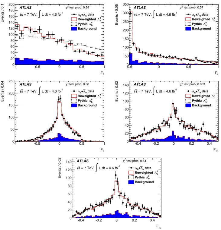
2 F -1 -0.5 0 0.5 1 Events / 0.1 0 20 40 60 80 100 120 140 160 180 200 data b Λ + b Λ 0 b Λ Reweighted 0 b Λ Pythia Background test prob: 0.98 2 χ ATLAS -1 L dt = 4.6 fb
∫
= 7 TeV, s 4 F -0.5 0 0.5 1 Events / 0.05 0 50 100 150 200 250 300 350 data b Λ + b Λ 0 b Λ Reweighted 0 b Λ Pythia Background test prob: 0.57 2 χ ATLAS -1 L dt = 4.6 fb∫
= 7 TeV, s 6 F -1 -0.5 0 0.5 1 Events / 0.04 0 50 100 150 200 250 data b Λ + b Λ 0 b Λ Reweighted 0 b Λ Pythia Background test prob: 0.80 2 χ ATLAS -1 L dt = 4.6 fb∫
= 7 TeV, s 18 F -0.4 -0.2 0 0.2 0.4 Events / 0.02 0 20 40 60 80 100 120 140 data b Λ + b Λ 0 b Λ Reweighted 0 b Λ Pythia Background test prob: 0.063 2 χ ATLAS -1 L dt = 4.6 fb∫
= 7 TeV, s 19 F -0.4 -0.2 0 0.2 0.4 Events / 0.02 0 20 40 60 80 100 120 140 data b Λ + b Λ 0 b Λ Reweighted 0 b Λ Pythia Background test prob: 0.64 2 χ ATLAS -1 L dt = 4.6 fb∫
= 7 TeV, sFIG. 6. The predicted distributions of Fi variables from the sum of the weighted MC events (red line) and the background
(blue area) are compared with data (black points). The background is estimated by adding the left and right sidebands and scaling by 0.5. The χ2-test probability of each comparison is shown in the top left corner of the plot. The predictions of the
unweighted MC events (black dashed line) are also shown.
Eq. (10). The fit is repeated and the new uncer-tainties in the fitted parameters are estimated, this time including the uncertainty from both the data and MC sample statistics. The default values of the statistical uncertainties are subtracted in quadra-ture from the new ones to isolate the contribution of the limited MC sample size. In case of the αb
pa-rameter, this uncertainty is estimated to be 0.047. • The value of αΛ, taken from Ref. [19], is varied by
one standard deviation to check the effect on the extracted parameters. The differences are taken as a systematic uncertainty, which is 0.009 for the value of αb.
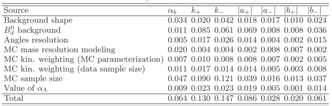
TABLE VI. Systematic uncertainties. Source αb k+ k− |a+| |a−| |b+| |b−| Background shape 0.034 0.020 0.042 0.018 0.017 0.010 0.024 B0 d background 0.011 0.085 0.061 0.069 0.008 0.008 0.036 Angles resolution 0.005 0.017 0.026 0.014 0.004 0.002 0.015
MC mass resolution modeling 0.020 0.004 0.004 0.002 0.008 0.007 0.002 MC kin. weighting (MC parameterization) 0.007 0.010 0.008 0.008 0.007 0.002 0.005 MC kin. weighting (data sample size) 0.011 0.017 0.014 0.014 0.005 0.003 0.008
MC sample size 0.047 0.090 0.121 0.039 0.016 0.013 0.037
Value of αΛ 0.009 0.023 0.023 0.019 0.005 0.001 0.014
Total 0.064 0.130 0.147 0.086 0.028 0.020 0.061
The contributions of these sources to the systematic un-certainties of the measured parameters are summarized in Table VI. The total systematic uncertainty is calcu-lated by adding individual contributions in quadrature. The total uncertainty for αb is 0.064.
VIII. CONCLUSIONS
A measurement of the parity-violating decay asymme-try parameter αb and the helicity amplitudes for the
de-cay Λ0b → J/ψ(µ+µ−)Λ0(pπ−) has been performed using
the 4.6 fb−1 pp collisions at a center-of-mass energy of
7 TeV recorded by the ATLAS detector at the LHC in 2011. The measured values of αb, k+ and k− are:
αb= 0.30 ± 0.16(stat) ± 0.06(syst),
k+= 0.21+0.14−0.21(stat) ± 0.13(syst),
k−= 0.13+0.20−0.13(stat) ± 0.15(syst), (18)
corresponding to the value of helicity parameters |a+| = 0.17+0.12−0.17(stat) ± 0.09(syst), |a−| = 0.59 +0.06 −0.07(stat) ± 0.03(syst), |b+| = 0.79+0.04−0.05(stat) ± 0.02(syst), |b−| = 0.08+0.13−0.08(stat) ± 0.06(syst). (19) The Λ0
b decay has large amplitudes |a−| and |b+|, which
means the negative-helicity states for Λ0 are preferred.
The Λ0 and J/ψ from Λ0
b decay are highly polarized.
Adding in quadrature the statistical and systematic un-certainties, the observed value of αbis consistent with the
recent measurement αb = 0.05 ± 0.17(stat) ± 0.07(syst)
by LHCb [14] at the level of one standard deviation. However, it is not consistent with the expectation from pQCD [11] (αb in the range from −0.17 to −0.14), and
HQET [12, 13] (αb = 0.78) at a level of about 2.6 and
2.8 standard deviations, respectively.
ACKNOWLEDGMENTS
We thank CERN for the very successful operation of the LHC, as well as the support staff from our institutions without whom ATLAS could not be operated efficiently. We acknowledge the support of ANPCyT, Argentina; YerPhI, Armenia; ARC, Australia; BMWF and FWF, Austria; ANAS, Azerbaijan; SSTC, Belarus; CNPq and FAPESP, Brazil; NSERC, NRC and CFI, Canada; CERN; CONICYT, Chile; CAS, MOST and NSFC, China; COLCIENCIAS, Colombia; MSMT CR, MPO CR and VSC CR, Czech Republic; DNRF, DNSRC and Lundbeck Foundation, Denmark; EPLANET, ERC and NSRF, European Union; IN2P3-CNRS, CEA-DSM/IRFU, France; GNSF, Georgia; BMBF, DFG, HGF, MPG and AvH Foundation, Germany; GSRT and NSRF, Greece; ISF, MINERVA, GIF, I-CORE and Benoziyo Center, Israel; INFN, Italy; MEXT and JSPS, Japan; CNRST, Morocco; FOM and NWO, Netherlands; BRF and RCN, Norway; MNiSW and NCN, Poland; GRICES and FCT, Portugal; MNE/IFA, Romania; MES of Russia and ROSATOM, Russian Federation; JINR; MSTD, Serbia; MSSR, Slovakia; ARRS and MIZˇS, Slove-nia; DST/NRF, South Africa; MINECO, Spain; SRC and Wallenberg Foundation, Sweden; SER, SNSF and Cantons of Bern and Geneva, Switzerland; NSC, Tai-wan; TAEK, Turkey; STFC, the Royal Society and Lev-erhulme Trust, United Kingdom; DOE and NSF, United States of America.
The crucial computing support from all WLCG part-ners is acknowledged gratefully, in particular from CERN and the ATLAS Tier-1 facilities at TRIUMF (Canada), NDGF (Denmark, Norway, Sweden), CC-IN2P3 (France), KIT/GridKA (Germany), INFN-CNAF (Italy), NL-T1 (Netherlands), PIC (Spain), ASGC (Tai-wan), RAL (UK) and BNL (USA) and in the Tier-2 fa-cilities worldwide.
Hud-son,Phys. Rev. 105, 1413 (1957).
[3] R. Garwin, L. Lederman, and M. Weinrich,Phys. Rev. 105, 1415 (1957).
[4] F. Eisler, R. Plano, A. Prodell, N. Samios, M. Schwartz, et al.,Phys. Rev. 108, 1353 (1957).
[5] J. W. Cronin and O. E. Overseth,Phys. Rev. 129, 1795 (1963).
[6] H.-Y. Cheng, Phys. Rev. D 56, 2799 (1997),
arXiv:hep-ph/9612223.
[7] Fayyazuddin and Riazuddin, Phys. Rev. D 58, 014016 (1998),arXiv:hep-ph/9802326.
[8] R. Mohanta, A. K. Giri, M. P. Khanna, M. Ishida, S. Ishida, et al., Prog. Theor. Phys. 101, 959 (1999),
arXiv:hep-ph/9904324.
[9] Z.-T. Wei, H.-W. Ke, and X.-Q. Li, Phys. Rev. D 80, 094016 (2009),arXiv:0909.0100.
[10] T. Gutsche, M. A. Ivanov, J. G. Korner, V. E. Lyubovit-skij, and P. Santorelli,Phys. Rev. D 88, 114018 (2013), arXiv:1309.7879.
[11] C.-H. Chou, H.-H. Shih, S.-C. Lee, and H.-n. Li,Phys.
Rev. D 65, 074030 (2002),arXiv:hep-ph/0112145.
[12] O. Leitner, Z. Ajaltouni, and E. Conte, Nucl. Phys.
A755, 435 (2005),arXiv:hep-ph/0412131.
[13] Z. Ajaltouni, E. Conte, and O. Leitner, Phys. Lett. B
614, 165 (2005),arXiv:hep-ph/0412116.
[14] R. Aaij et al. (LHCb Collaboration),Phys. Lett. B 724, 27 (2013),arXiv:1302.5578.
[15] J. Hrivnac, R. Lednicky, and M. Smizanska,J. Phys. G 21, 629 (1995),arXiv:hep-ph/9405231.
[16] ATLAS uses a right-handed coordinate system with its origin at the nominal interaction point (IP) in the cen-ter of the detector and the z-axis along the beam pipe.
The x-axis points from the IP to the center of the LHC ring, and the y-axis points upward. Cylindrical coordi-nates (r, Φ) are used in the transverse plane, Φ being the azimuthal angle around the beam pipe. The pseu-dorapidity is defined in terms of the polar angle Θ as η = − ln tan(Θ/2).
[17] R. Lednicky, Sov. J. Nucl. Phys. 43, 817 (1986). [18] P. Bialas, J. Korner, M. Kramer, and K. Zalewski, Z.
Phys. C 57, 115 (1993).
[19] J. Beringer et al. (Particle Data Group), Phys. Rev. D 86, 010001 (2012).
[20] ATLAS Collaboration,JINST 3, S08003 (2008). [21] ATLAS Collaboration,Eur. Phys. J. C 73, 2518 (2013),
arXiv:1302.4393.
[22] ATLAS Collaboration,Eur. Phys. J. C 72, 1849 (2012), arXiv:1110.1530.
[23] T. Sjostrand, S. Mrenna, and P. Z. Skands,J. High
En-ergy Phys. 05 (2006) 026,arXiv:hep-ph/0603175.
[24] ATLAS Collaboration,Eur. Phys. J. C 70, 823 (2010), arXiv:1005.4568.
[25] S. Agostinelli et al. (GEANT4 Collaboration),Nucl.
In-strum. Methods Phys. Res., Sect. A 506, 250 (2003).
[26] ATLAS Collaboration, Phys. Lett. B 707, 438 (2012), arXiv:1109.0525.
[27] V. Kostyukhin, Report No. ATL-PHYS-2003-031, 2003, http://cds.cern.ch/record/685551.
[28] ATLAS Collaboration,Phys. Rev. D 87, 032002 (2013), arXiv:1207.2284.
[29] K. S. Cranmer, Comput. Phys. Commun. 136, 198 (2001),arXiv:hep-ex/0011057.
[30] W. Verkerke and D. P. Kirkby, eConf C0303241, MOLT007 (2003),arXiv:physics/0306116.
The ATLAS Collaboration
G. Aad84, T. Abajyan21, B. Abbott112, J. Abdallah152, S. Abdel Khalek116, O. Abdinov11, R. Aben106, B. Abi113,
M. Abolins89, O.S. AbouZeid159, H. Abramowicz154, H. Abreu137, Y. Abulaiti147a,147b, B.S. Acharya165a,165b,a,
L. Adamczyk38a, D.L. Adams25, J. Adelman177, S. Adomeit99, T. Adye130, T. Agatonovic-Jovin13b,
J.A. Aguilar-Saavedra125f,125a, M. Agustoni17, S.P. Ahlen22, A. Ahmad149, F. Ahmadov64,b, G. Aielli134a,134b,
T.P.A. ˚Akesson80, G. Akimoto156, A.V. Akimov95, J. Albert170, S. Albrand55, M.J. Alconada Verzini70,
M. Aleksa30, I.N. Aleksandrov64, C. Alexa26a, G. Alexander154, G. Alexandre49, T. Alexopoulos10,
M. Alhroob165a,165c, G. Alimonti90a, L. Alio84, J. Alison31, B.M.M. Allbrooke18, L.J. Allison71, P.P. Allport73,
S.E. Allwood-Spiers53, J. Almond83, A. Aloisio103a,103b, R. Alon173, A. Alonso36, F. Alonso70, C. Alpigiani75,
A. Altheimer35, B. Alvarez Gonzalez89, M.G. Alviggi103a,103b, K. Amako65, Y. Amaral Coutinho24a, C. Amelung23,
D. Amidei88, V.V. Ammosov129,∗, S.P. Amor Dos Santos125a,125c, A. Amorim125a,125b, S. Amoroso48, N. Amram154,
G. Amundsen23, C. Anastopoulos140, L.S. Ancu17, N. Andari30, T. Andeen35, C.F. Anders58b, G. Anders30,
K.J. Anderson31, A. Andreazza90a,90b, V. Andrei58a, X.S. Anduaga70, S. Angelidakis9, P. Anger44, A. Angerami35,
F. Anghinolfi30, A.V. Anisenkov108, N. Anjos125a, A. Annovi47, A. Antonaki9, M. Antonelli47, A. Antonov97,
J. Antos145b, F. Anulli133a, M. Aoki65, L. Aperio Bella18, R. Apolle119,c, G. Arabidze89, I. Aracena144, Y. Arai65,
J.P. Araque125a, A.T.H. Arce45, J-F. Arguin94, S. Argyropoulos42, M. Arik19a, A.J. Armbruster30, O. Arnaez82,
V. Arnal81, O. Arslan21, A. Artamonov96, G. Artoni23, S. Asai156, N. Asbah94, A. Ashkenazi154, S. Ask28,
B. ˚Asman147a,147b, L. Asquith6, K. Assamagan25, R. Astalos145a, M. Atkinson166, N.B. Atlay142, B. Auerbach6,
E. Auge116, K. Augsten127, M. Aurousseau146b, G. Avolio30, G. Azuelos94,d, Y. Azuma156, M.A. Baak30,
C. Bacci135a,135b, H. Bachacou137, K. Bachas155, M. Backes30, M. Backhaus30, J. Backus Mayes144, E. Badescu26a,
P. Bagiacchi133a,133b, P. Bagnaia133a,133b, Y. Bai33a, D.C. Bailey159, T. Bain35, J.T. Baines130, O.K. Baker177,
S. Baker77, P. Balek128, F. Balli137, E. Banas39, Sw. Banerjee174, D. Banfi30, A. Bangert151, A.A.E. Bannoura176, V. Bansal170, H.S. Bansil18, L. Barak173, S.P. Baranov95, T. Barber48, E.L. Barberio87, D. Barberis50a,50b,
M. Barbero84, T. Barillari100, M. Barisonzi176, T. Barklow144, N. Barlow28, B.M. Barnett130, R.M. Barnett15,
Z. Barnovska5, A. Baroncelli135a, G. Barone49, A.J. Barr119, F. Barreiro81, J. Barreiro Guimar˜aes da Costa57,
R. Bartoldus144, A.E. Barton71, P. Bartos145a, V. Bartsch150, A. Bassalat116, A. Basye166, R.L. Bates53,
L. Batkova145a, J.R. Batley28, M. Battistin30, F. Bauer137, H.S. Bawa144,e, T. Beau79, P.H. Beauchemin162,
R. Beccherle123a,123b, P. Bechtle21, H.P. Beck17, K. Becker176, S. Becker99, M. Beckingham139, C. Becot116,
A.J. Beddall19c, A. Beddall19c, S. Bedikian177, V.A. Bednyakov64, C.P. Bee149, L.J. Beemster106, T.A. Beermann176,
M. Begel25, K. Behr119, C. Belanger-Champagne86, P.J. Bell49, W.H. Bell49, G. Bella154, L. Bellagamba20a,
A. Bellerive29, M. Bellomo85, A. Belloni57, O.L. Beloborodova108,f, K. Belotskiy97, O. Beltramello30, O. Benary154,
D. Benchekroun136a, K. Bendtz147a,147b, N. Benekos166, Y. Benhammou154, E. Benhar Noccioli49,
J.A. Benitez Garcia160b, D.P. Benjamin45, J.R. Bensinger23, K. Benslama131, S. Bentvelsen106, D. Berge106,
E. Bergeaas Kuutmann16, N. Berger5, F. Berghaus170, E. Berglund106, J. Beringer15, C. Bernard22, P. Bernat77,
C. Bernius78, F.U. Bernlochner170, T. Berry76, P. Berta128, C. Bertella84, F. Bertolucci123a,123b, M.I. Besana90a,
G.J. Besjes105, O. Bessidskaia147a,147b, N. Besson137, C. Betancourt48, S. Bethke100, W. Bhimji46, R.M. Bianchi124,
L. Bianchini23, M. Bianco30, O. Biebel99, S.P. Bieniek77, K. Bierwagen54, J. Biesiada15, M. Biglietti135a,
J. Bilbao De Mendizabal49, H. Bilokon47, M. Bindi54, S. Binet116, A. Bingul19c, C. Bini133a,133b, C.W. Black151,
J.E. Black144, K.M. Black22, D. Blackburn139, R.E. Blair6, J.-B. Blanchard137, T. Blazek145a, I. Bloch42,
C. Blocker23, W. Blum82,∗, U. Blumenschein54, G.J. Bobbink106, V.S. Bobrovnikov108, S.S. Bocchetta80, A. Bocci45,
C.R. Boddy119, M. Boehler48, J. Boek176, T.T. Boek176, J.A. Bogaerts30, A.G. Bogdanchikov108, A. Bogouch91,∗,
C. Bohm147a, J. Bohm126, V. Boisvert76, T. Bold38a, V. Boldea26a, A.S. Boldyrev98, N.M. Bolnet137, M. Bomben79,
M. Bona75, M. Boonekamp137, A. Borisov129, G. Borissov71, M. Borri83, S. Borroni42, J. Bortfeldt99,
V. Bortolotto135a,135b, K. Bos106, D. Boscherini20a, M. Bosman12, H. Boterenbrood106, J. Boudreau124, J. Bouffard2,
E.V. Bouhova-Thacker71, D. Boumediene34, C. Bourdarios116, N. Bousson113, S. Boutouil136d, A. Boveia31,
J. Boyd30, I.R. Boyko64, I. Bozovic-Jelisavcic13b, J. Bracinik18, P. Branchini135a, A. Brandt8, G. Brandt15,
O. Brandt58a, U. Bratzler157, B. Brau85, J.E. Brau115, H.M. Braun176,∗, S.F. Brazzale165a,165c, B. Brelier159,
K. Brendlinger121, A.J. Brennan87, R. Brenner167, S. Bressler173, K. Bristow146c, T.M. Bristow46, D. Britton53,
F.M. Brochu28, I. Brock21, R. Brock89, C. Bromberg89, J. Bronner100, G. Brooijmans35, T. Brooks76,
W.K. Brooks32b, J. Brosamer15, E. Brost115, G. Brown83, J. Brown55, P.A. Bruckman de Renstrom39,
D. Bruncko145b, R. Bruneliere48, S. Brunet60, A. Bruni20a, G. Bruni20a, M. Bruschi20a, L. Bryngemark80,
T. Buanes14, Q. Buat143, F. Bucci49, P. Buchholz142, R.M. Buckingham119, A.G. Buckley53, S.I. Buda26a,
I.A. Budagov64, F. Buehrer48, L. Bugge118, M.K. Bugge118, O. Bulekov97, A.C. Bundock73, H. Burckhart30,
S. Burdin73, B. Burghgrave107, S. Burke130, I. Burmeister43, E. Busato34, V. B¨uscher82, P. Bussey53, C.P. Buszello167, B. Butler57, J.M. Butler22, A.I. Butt3, C.M. Buttar53, J.M. Butterworth77, P. Butti106,
W. Buttinger28, A. Buzatu53, M. Byszewski10, S. Cabrera Urb´an168, D. Caforio20a,20b, O. Cakir4a, P. Calafiura15,
S. Camarda42, D. Cameron118, L.M. Caminada15, R. Caminal Armadans12, S. Campana30, M. Campanelli77,
A. Campoverde149, V. Canale103a,103b, A. Canepa160a, J. Cantero81, R. Cantrill76, T. Cao40,
M.D.M. Capeans Garrido30, I. Caprini26a, M. Caprini26a, M. Capua37a,37b, R. Caputo82, R. Cardarelli134a,
T. Carli30, G. Carlino103a, L. Carminati90a,90b, S. Caron105, E. Carquin32a, G.D. Carrillo-Montoya146c,
A.A. Carter75, J.R. Carter28, J. Carvalho125a,125c, D. Casadei77, M.P. Casado12, E. Castaneda-Miranda146b,
A. Castelli106, V. Castillo Gimenez168, N.F. Castro125a, P. Catastini57, A. Catinaccio30, J.R. Catmore71,
A. Cattai30, G. Cattani134a,134b, S. Caughron89, V. Cavaliere166, D. Cavalli90a, M. Cavalli-Sforza12,
V. Cavasinni123a,123b, F. Ceradini135a,135b, B. Cerio45, K. Cerny128, A.S. Cerqueira24b, A. Cerri150, L. Cerrito75,
F. Cerutti15, M. Cerv30, A. Cervelli17, S.A. Cetin19b, A. Chafaq136a, D. Chakraborty107, I. Chalupkova128,
K. Chan3, P. Chang166, B. Chapleau86, J.D. Chapman28, D. Charfeddine116, D.G. Charlton18, C.C. Chau159,
C.A. Chavez Barajas150, S. Cheatham86, A. Chegwidden89, S. Chekanov6, S.V. Chekulaev160a, G.A. Chelkov64,
M.A. Chelstowska88, C. Chen63, H. Chen25, K. Chen149, L. Chen33d,g, S. Chen33c, X. Chen146c, Y. Chen35,
H.C. Cheng88, Y. Cheng31, A. Cheplakov64, R. Cherkaoui El Moursli136e, V. Chernyatin25,∗, E. Cheu7,
L. Chevalier137, V. Chiarella47, G. Chiefari103a,103b, J.T. Childers6, A. Chilingarov71, G. Chiodini72a,
A.S. Chisholm18, R.T. Chislett77, A. Chitan26a, M.V. Chizhov64, S. Chouridou9, B.K.B. Chow99, I.A. Christidi77,
D. Chromek-Burckhart30, M.L. Chu152, J. Chudoba126, L. Chytka114, G. Ciapetti133a,133b, A.K. Ciftci4a, R. Ciftci4a,
D. Cinca62, V. Cindro74, A. Ciocio15, P. Cirkovic13b, Z.H. Citron173, M. Citterio90a, M. Ciubancan26a, A. Clark49,
P.J. Clark46, R.N. Clarke15, W. Cleland124, J.C. Clemens84, B. Clement55, C. Clement147a,147b, Y. Coadou84,
M. Cobal165a,165c, A. Coccaro139, J. Cochran63, L. Coffey23, J.G. Cogan144, J. Coggeshall166, B. Cole35, S. Cole107,
A.P. Colijn106, C. Collins-Tooth53, J. Collot55, T. Colombo58c, G. Colon85, G. Compostella100,
P. Conde Mui˜no125a,125b, E. Coniavitis167, M.C. Conidi12, S.H. Connell146b, I.A. Connelly76, S.M. Consonni90a,90b, V. Consorti48, S. Constantinescu26a, C. Conta120a,120b, G. Conti57, F. Conventi103a,h, M. Cooke15, B.D. Cooper77,
A.M. Cooper-Sarkar119, N.J. Cooper-Smith76, K. Copic15, T. Cornelissen176, M. Corradi20a, F. Corriveau86,i,
A. Corso-Radu164, A. Cortes-Gonzalez12, G. Cortiana100, G. Costa90a, M.J. Costa168, D. Costanzo140, D. Cˆot´e8,
G. Cottin28, G. Cowan76, B.E. Cox83, K. Cranmer109, G. Cree29, S. Cr´ep´e-Renaudin55, F. Crescioli79,
M. Crispin Ortuzar119, M. Cristinziani21, G. Crosetti37a,37b, C.-M. Cuciuc26a, C. Cuenca Almenar177,
T. Cuhadar Donszelmann140, J. Cummings177, M. Curatolo47, C. Cuthbert151, H. Czirr142, P. Czodrowski3, Z. Czyczula177, S. D’Auria53, M. D’Onofrio73, M.J. Da Cunha Sargedas De Sousa125a,125b, C. Da Via83,
W. Dabrowski38a, A. Dafinca119, T. Dai88, O. Dale14, F. Dallaire94, C. Dallapiccola85, M. Dam36, A.C. Daniells18,
M. Dano Hoffmann137, V. Dao105, G. Darbo50a, G.L. Darlea26c, S. Darmora8, J.A. Dassoulas42, W. Davey21,
C. David170, T. Davidek128, E. Davies119,c, M. Davies94, O. Davignon79, A.R. Davison77, P. Davison77,
Y. Davygora58a, E. Dawe143, I. Dawson140, R.K. Daya-Ishmukhametova23, K. De8, R. de Asmundis103a, S. De Castro20a,20b, S. De Cecco79, J. de Graat99, N. De Groot105, P. de Jong106, C. De La Taille116,
H. De la Torre81, F. De Lorenzi63, L. De Nooij106, D. De Pedis133a, A. De Salvo133a, U. De Sanctis165a,165c,
A. De Santo150, J.B. De Vivie De Regie116, G. De Zorzi133a,133b, W.J. Dearnaley71, R. Debbe25, C. Debenedetti46,
B. Dechenaux55, D.V. Dedovich64, J. Degenhardt121, I. Deigaard106, J. Del Peso81, T. Del Prete123a,123b,
F. Deliot137, C.M. Delitzsch49, M. Deliyergiyev74, A. Dell’Acqua30, L. Dell’Asta22, M. Dell’Orso123a,123b,
M. Della Pietra103a,h, D. della Volpe49, M. Delmastro5, P.A. Delsart55, C. Deluca106, S. Demers177, M. Demichev64,
A. Demilly79, S.P. Denisov129, D. Derendarz39, J.E. Derkaoui136d, F. Derue79, P. Dervan73, K. Desch21,
C. Deterre42, P.O. Deviveiros106, A. Dewhurst130, S. Dhaliwal106, A. Di Ciaccio134a,134b, L. Di Ciaccio5,
A. Di Domenico133a,133b, C. Di Donato103a,103b, A. Di Girolamo30, B. Di Girolamo30, A. Di Mattia153,
B. Di Micco135a,135b, R. Di Nardo47, A. Di Simone48, R. Di Sipio20a,20b, D. Di Valentino29, M.A. Diaz32a,
E.B. Diehl88, J. Dietrich42, T.A. Dietzsch58a, S. Diglio87, A. Dimitrievska13a, J. Dingfelder21, C. Dionisi133a,133b, P. Dita26a, S. Dita26a, F. Dittus30, F. Djama84, T. Djobava51b, M.A.B. do Vale24c, A. Do Valle Wemans125a,125g,
T.K.O. Doan5, D. Dobos30, E. Dobson77, C. Doglioni49, T. Doherty53, T. Dohmae156, J. Dolejsi128, Z. Dolezal128,
B.A. Dolgoshein97,∗, M. Donadelli24d, S. Donati123a,123b, P. Dondero120a,120b, J. Donini34, J. Dopke30, A. Doria103a,
A. Dos Anjos174, M.T. Dova70, A.T. Doyle53, M. Dris10, J. Dubbert88, S. Dube15, E. Dubreuil34, E. Duchovni173,
G. Duckeck99, O.A. Ducu26a, D. Duda176, A. Dudarev30, F. Dudziak63, L. Duflot116, L. Duguid76, M. D¨uhrssen30,
M. Dunford58a, H. Duran Yildiz4a, M. D¨uren52, A. Durglishvili51b, M. Dwuznik38a, M. Dyndal38a, J. Ebke99,
W. Edson2, N.C. Edwards46, W. Ehrenfeld21, T. Eifert144, G. Eigen14, K. Einsweiler15, T. Ekelof167,
M. El Kacimi136c, M. Ellert167, S. Elles5, F. Ellinghaus82, N. Ellis30, J. Elmsheuser99, M. Elsing30,
D. Emeliyanov130, Y. Enari156, O.C. Endner82, M. Endo117, R. Engelmann149, J. Erdmann177, A. Ereditato17,
D. Eriksson147a, G. Ernis176, J. Ernst2, M. Ernst25, J. Ernwein137, D. Errede166, S. Errede166, E. Ertel82,
M. Escalier116, H. Esch43, C. Escobar124, B. Esposito47, A.I. Etienvre137, E. Etzion154, H. Evans60, L. Fabbri20a,20b, G. Facini30, R.M. Fakhrutdinov129, S. Falciano133a, Y. Fang33a, M. Fanti90a,90b, A. Farbin8, A. Farilla135a,
T. Farooque12, S. Farrell164, S.M. Farrington171, P. Farthouat30, F. Fassi168, P. Fassnacht30, D. Fassouliotis9,
A. Favareto50a,50b, L. Fayard116, P. Federic145a, O.L. Fedin122,j, W. Fedorko169, M. Fehling-Kaschek48, S. Feigl30,