Development and Application of Statistical Methods to
Support Air Quality Policy Decisions
José Carlos Magalhães Pires
Graduated in Chemical Engineering
by the Faculty of Engineering of the University of Porto
Dissertation submitted to obtain the degree of Doctor of Philosophy in Environmental Engineering
Development and Application of Statistical Methods to
Support Air Quality Policy Decisions
José Carlos Magalhães Pires
Supervision
Fernando Gomes Martins (PhD) and Maria do Carmo da Silva Pereira (PhD) Department of Chemical Engineering, Faculty of Engineering, University of Porto
Abstract
It is well known the health effects associated with air pollution. Several studies were published, showing an increasing awareness among the scientific community and policy makers about public health problems due to exposure to air pollution. Policy makers require more detailed air quality information to take measures to reduce the effects on health and to improve the air quality management. This thesis aims to develop procedures using statistical methods to support a broad range of policy decisions concerning this subject.
The first aim was the application of statistical methods, such as principal component analysis and cluster analysis, to characterize the air pollution behaviours in an urban area allowing the identification of monitoring sites with redundant air quality measurements. These measurements represent a loss of profitability of the air quality monitoring network resources. Accordingly, the application of these statistical methods let the following policy decisions: (i) remove the redundant monitoring sites, reducing the costs of the equipment maintenance; or (ii) move the redundant monitoring sites to other places increasing the area of monitored region. The air pollutant concentrations at the removed sites can be estimated with statistical models using the concentrations measured at the remaining sites. Moreover, the air pollution behaviours are related with the location of emission sources. The possible location of important sources of air pollutants was also determined through the analysis of variation of their concentrations with the wind direction. Concerning the characterization of the air pollution behaviours, the actual distribution of monitoring sites in the air quality monitoring network of Oporto Metropolitan Area presented several redundant measurements. The number of monitoring sites could be reduced at about 50% in some of the analysed air pollutants. Several air pollution sources were identified with the analysis of the variation of the air pollutant concentrations with the wind
affecting all monitoring sites during the analysed period.
The second aim of this thesis was the development of statistical models to predict the concentrations of air pollutants (O3 and PM10) of the next day. Several models
were applied, including linear and non-linear ones. As far as the author knows, independent component regression, partial least squares regression, stepwise artificial neural networks, threshold regression and genetic programming were applied for the first time in this field. Besides prediction of the air pollutant concentrations, these models selected the important variables (environmental and meteorological) that influence these values, which is an useful information for the air quality management. The linear models had an advantage of taking less computational time than the other models. Taking into account the performance of these models, quantile regression presented better results in the training period, as it tries to model the entire distribution of the dependent variable. However, this model presented worse performance in the test period. The linear model with best predictive performance was the partial least squares regression. Despite having longer computation time, the non-linear models predicted better than the linear ones, specially the models using the evolutionary procedure for their determination. Threshold regression using genetic algorithms and genetic programming for O3 and multi-gene genetic programming for PM10 were the
models with better predictive performance.
Keywords: air quality management, statistical methods, air quality modelling,
Os efeitos negativos associados à poluição do ar são bem conhecidos. Muitos estudos foram publicados, apresentando uma crescente preocupação da comunidade científica e dos decisores políticos relativamente aos problemas de saúde pública causados pela poluição do ar. Os decisores políticos necessitam de informação mais detalhada sobre a qualidade do ar de modo a tomar medidas de redução dos seus efeitos na saúde e melhorar a gestão da qualidade do ar. Este trabalho tem como principal objectivo o desenvolvimento de procedimentos usando métodos estatísticos para apoio de decisões políticas relacionadas com este tema.
A aplicação de métodos estatísticos, tais como a análise de componentes principais e análise de agrupamentos, permitiu a caracterização da variação da concentração dos poluentes atmosféricos numa região urbana e, ao mesmo tempo, a identificação de locais de monitorização com medições redundantes. Estas medições representam uma perda de rentabilidade dos recursos das redes de monitorização da qualidade do ar. Deste modo, a aplicação dos referidos métodos estatísticos pode suportar as seguintes decisões: (i) eliminar as estações de monitorização com medições redundantes, reduzindo os custos relativos à manutenção do respectivo equipamento; ou (ii) deslocalizar as referidas estações para outros locais, aumentando a área da região monitorizada. As concentrações de poluentes nos locais em que se pode desactivar as estações podem ser estimadas com modelos estatísticos usando os valores medidos nas restantes estações de monitorização. A variação das concentrações dos poluentes atmosféricos está relacionada com a localização relativa de fontes de emissão dos respectivos poluentes. A possível localização de importantes fontes de emissão foi determinada através da análise da variação da concentração de poluentes com a direcção do vento. Caracterizando as variações observadas pelas concentrações dos poluentes analisados, verificou-se que a distribuição das estações na rede de
redundantes. O número de locais de monitorização pode, para alguns poluentes, ser reduzido para metade. Várias fontes de emissão foram identificadas com a análise da variação da concentração de poluentes com a direcção do vento. A mais importante esteve localizada fora da região definida pela rede de monitorização na direcção E-SE, afectando todas as estações durante o período analisado.
Vários modelos estatísticos (lineares e não lineares) foram desenvolvidos para prever as concentrações dos poluentes atmosféricos (O3 e PM10). Tanto quanto se
sabe, a regressão por componentes independentes, a regressão por mínimos quadrados parciais, as redes neuronais artificiais desenvolvidas passo a passo, a regressão com limiares e a programação genética foram técnicas de modelização aplicadas pela primeira vez nesta área. Além de prever as concentrações de poluentes atmosféricos, estes modelos seleccionam variáveis importantes (concentrações de outros poluentes ou variáveis meteorológicas) que influenciam esses valores, sendo uma informação útil para a gestão da qualidade do ar. Os modelos lineares têm a vantagem de necessitar de menos tempo de computação do que os modelos não lineares. Tendo em conta os desempenhos destes modelos, a regressão por percentis teve melhores resultados no período de treino, uma vez que o modelo tenta descrever toda a distribuição da variável dependente. No entanto, este modelo teve pior desempenho na etapa de previsão. O modelo linear com melhor desempenho na previsão foi a regressão por mínimos quadrados parciais. Apesar de ter maior tempo de computação, os modelos não lineares prevêem melhor que os modelos lineares, especialmente quando usam o procedimento evolucionário na sua determinação. Assim, os modelos com limiares usando algoritmos genéticos e programação genética para o O3 e programação genética
com múltiplos genes para PM10 foram os que apresentaram os melhores
desempenhos.
Palavras-chave: qualidade do ar, métodos estatísticos, modelização da qualidade
Les effets négatifs associés à la pollution de l’air sont bien connus. Plusieurs études ont été publiées montrant la préoccupation croissante de la communauté scientifique et des décideurs politiques concernant les problèmes de santé publique causés par la pollution de l’air. Les décideurs politiques ont la nécessité d’avoir une information plus détaillée de la qualité de l’air afin de pouvoir prendre des mesures de réduction de ces effets sur la santé et améliorer la gestion de la qualité de l’air. Ce travail a pour principal objectif le développement de procédures utilisant des méthodes statistiques de forme a soutenir les décisions politiques liées à ce sujet.
L’application de méthodes statistiques, telles que l’analyse en composantes principales et l’analyse de grappes, a permis la caractérisation de la variation de la concentration des polluants atmosphériques dans une zones urbaines ainsi que l’identification de sites de surveillance avec des mesures redondantes. Ces mesures représentent une perte de rentabilité des ressources des réseaux de surveillance de la qualité de l’air. Ainsi, l’application de ces methodes statistiques peuvent appuyer les decisions politiques suivantes: (i) éliminer les sations de surveillance avec des mesures redondantes, reduisant le coût d’entretien des equipements; ou (ii) déplacer ces stations à d’autres endroits, augmentant l’aire de la region controlée. Les concentrations de polluants dans les endroits oú l’on peut désactiver les sations peuvent être estimés à l’aide de modèles statistiques utilisant les valeurs moyennes mesurées dans les autres sations de surveillance. La variation des concentrations des polluants atmosphériques est liée à la localisation relative des sources d’émission des polluents respectifs. Le possible emplacement de sources importantes de polluants a également éte déterminé par l’analyse de la variation de leurs concentrations avec la direction du vent. À travers la caractérisation des variations observées par les concentrations de polluants analysés, il a été constaté que la distribution des sites dans les réseau de surveillance de la zone
sites de surveillance peut, pour certains polluants, être réduit de moitié. Plusieurs sources d’émissions ont été identifiés à travers l’analyse de la variation de la concentraction de polluants avec la direction du vent. La plus importante était située à l’extérieur de la region définie par le réseau de surveillance dans la direction E-SE, affectant l’ensemble des stations au cours de la période analysée.
Plusieurs modèles statistiques, linéaires et non linéaires, ont été développés afin de prévoir les concentrations de polluants atmosphériques (O3 e PM10). Pour autant
qu’il se sache, la régression par composants indépendants, la régression des moindres carrés partiels, les réseaux neuronaux artificiels développés pas à pas, la régression avec des seuils et la programmation génétique ont été des techniques de modélisation appliquées pour la première fois dans ce domaine. En plus de pévoir les concentrations de polluants atmosphériques, ces modèles sélectionnent des variables importantes qui influent sur ces valeurs, étant ainsi une information utile pour la gestion de la qualité de l’air. Les modèles linéaires ont l’avantage d’exiger moins de temps de calcul que les modèles non linéaires. Compte tenu de la performance de ces modèles, la régression quantile a présenté de meilleurs résultats au cours de la période d’essai, une fois que le modèle tente de décrire l’ensemble de la distribution de la variable dépendante. Toutefois, ce modèles présente une pire performance prédictive. Le modèle linéaire ayant la meilleure performance en matière de prévision est la régression des moindres carrés partiels. Bien qu’ayant un temps de calcul superieur, les modèles non linéaires prédisent mieux que les modéles linéaires, en particulier ceux utilisant le processus d’évolution dans sa détermination. Ainsi, les modèles avec des seuils utilisant des algorithmes génétiques et la programmation génétique pour le O3 et la
programmation génétiques avec multiples genes pour PM10 ont été ceux présentant
les meilleures performances.
Mots-clés: qualité de l’air, méthodes statistiques, modélisation de la qualité de
I am grateful to my supervisors Fernando Gomes Martins (PhD) and Maria do Carmo da Silva Pereira (PhD), for introducing me this research topic and then providing me the necessary support. I also wish to thank Maria da Conceição Machado Alvim Ferraz (PhD) for her advice, suggestions and for sharing her knowledge in air quality with me. I can not forget the important suggestions and contributions of Joana, Sofia and Elodie in the preparation of this manuscript.
I also acknowledge: (i) the Faculdade de Engenharia da Universidade do Porto, the Departamento de Engenharia Química and Laboratório de Engenharia de
Processos, Ambiente e Energia for providing all the necessary facilities to perform
my studies; (ii) the Fundação para a Ciência e a Tecnologia for the fellowship SFRH/BD/23302/2005; and (iii) the Comissão de Coordenação e Desenvolvimento Regional do Norte and the Instituto Geofísico da Universidade do Porto for kindly providing the air quality and meteorological data.
At the end, I want to thank my family, Nádia and my friends for the support, patience and encouragement during this period.
To my family To Nádia To my friends
Table of Contents
Abstract ...V Resumo ...VII Résumé ... IX Acknowledgements... XI Table of Contents ... XIII Figure Index... XVI Table Index ... XIX List of Abbreviations... XXIII Notation ... XXVI
1. Introduction ...1
1.1. Scientific relevance...1
1.2. Thesis structure ...2
Part I. Management of Air Quality Monitoring Networks 2. Air Quality Evaluation in Oporto Metropolitan Area ...7
2.1. Sulphur dioxide...7
2.2. Particulate matter ...9
2.3. Carbon monoxide...9
2.4. Nitrogen oxides...10
2.5. Ozone ...11
2.6. Air quality data ...13
2.7. Exceedances to EU limits ...14
2.8. Conclusions...21
3. Characterization of Air Pollution Behaviours ...23
3.1. Introduction...23
3.2. Air quality data ...25
3.3. Results and discussion ...25
4.1. Introduction... 49
4.2. Air quality data... 50
4.3. Results and discussion... 51
4.4. Conclusions... 57
Part II. Prediction of Air Pollutant Concentrations 5. Prediction using statistical models ... 63
5.1. State of the art ... 63
5.2. Models applied in this thesis ... 66
6. Linear models... 67
6.1. Multiple linear regression ... 67
6.2. Principal component regression ... 69
6.3. Independent component regression... 71
6.4. Partial least squares regression... 72
6.5. Quantile regression... 73
6.6. Statistical significance of regression parameters ... 74
6.7. Performance indexes ... 75
6.8. Data ... 76
6.9. Results and discussion... 77
6.10. Conclusions... 83
7. Stepwise artificial neural networks ... 85
7.1. Introduction... 85
7.2. Stepwise artificial neural networks ... 88
7.3. Data ... 92
7.4. Results and discussion... 93
7.5. Conclusions... 97
8. Threshold regression models ... 99
8.1. Introduction... 99
8.2. Genetic algorithms and TR-GA procedure ... 100
8.5. Conclusions...106
9. Genetic Programming ...109
9.1. Introduction...109
9.2. Genetic programming ...110
9.3. Data...114
9.4. Results and discussion ...115
9.5. Conclusions...119
10. Multi-gene Genetic Programming ...121
10.1. Introduction...121
10.2. Data...122
10.3. Results and discussion ...123
10.4. Conclusions...128
11. Final Words ...129
11.1. General conclusions ...129
11.2. Future work...132
Figure 2.1 Location of the monitoring sites in the map of Oporto-MA (from Google Earth). ... 15
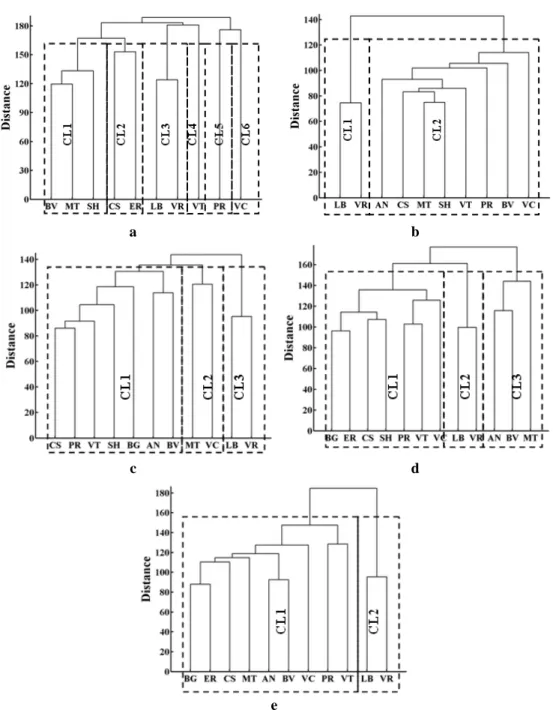
Figure 3.1 Dendrograms resulting from the application of CA to the (a) SO2,
(b) PM10, (c) CO, (d) NO2 and (e) O3 concentrations... 28
Figure 3.2 Average daily profile of the hourly average SO2 concentrations at
the monitoring sites grouped by the correspondent PC/CL category: (a) PC1/CL1, (b) PC2/CL3, (c) PC3/CL5, (d) PC4/CL2, (e) PC5/CL4 and (f) PC6/CL6. ... 30
Figure 3.3 Average daily profile of the hourly average PM10 concentrations for
the monitoring sites grouped by the correspondent PC/CL category: (a) PC1/CL2 and (b) PC2/CL1. ... 31
Figure 3.4 Average daily profile of the hourly mean CO concentrations for the monitoring sites grouped by the correspondent PC/CL category: (a) PC1/CL1, (b) PC2/CL3, and (c) PC3/CL2. ... 32
Figure 3.5 Average daily profile of the hourly average NO2 concentrations for
the monitoring sites grouped by the correspondent PC/CL category: (a) PC1/CL1, (b) PC2/CL2, and (c) PC1/CL3. ... 33
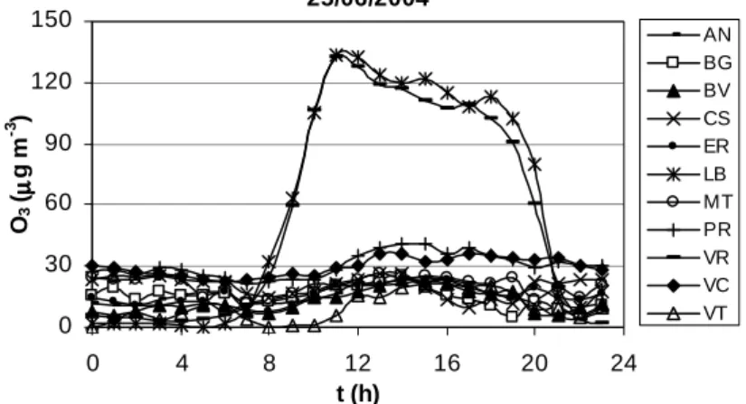
Figure 3.6 Average daily profile of the hourly average O3 concentrations for the
monitoring sites grouped by the correspondent PC/CL category: (a) PC1/CL1 and (b) PC2/CL2... 34
Figure 3.7 Relative frequency (%) of the direction from which the wind was blowing when hourly average concentrations of SO2 above 125 µg m
-3
were collected (number of occurrences in brackets). ... 36
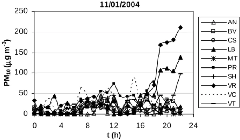
Figure 3.8 Relative frequency (%) of the direction from which the wind was blowing when hourly average concentrations of PM10 increased at least 50 µg
m-3 during the period that lasted from 17 to the 22 hours (number of occurrences in brackets). ... 37
Figure 3.9 Example of the profile of the hourly average PM10 concentrations when
(number of occurrences in brackets). ...40
Figure 3.11 Examples of the daily profiles of CO concentrations when the wind blew predominantly from: (a) NE-E, and (b) NW-N direction sectors. ...41
Figure 3.12 Relative frequency (%) of the direction from which the wind was blowing when hourly average NO2 concentration above 100 µg m
-3
was collected (number of occurrences in brackets)...42
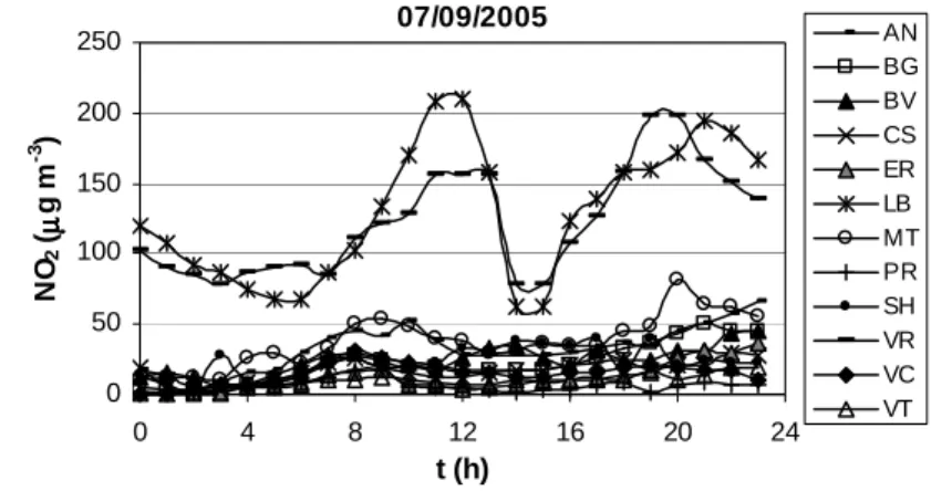
Figure 3.13 Example of the daily profile of NO2 concentrations when the wind
blew predominantly from NW-N direction sector...43
Figure 3.14 Relative frequency (%) of the direction from which the wind was blowing when hourly average O3 concentration above 120 µg m
-3
was collected (number of occurrences in brackets). ...44
Figure 3.15 Example of the daily profile of O3 concentrations when the wind
blew predominantly from W-NW direction sector...45
Figure 3.16 Example of the daily profile of NO2 concentrations...46
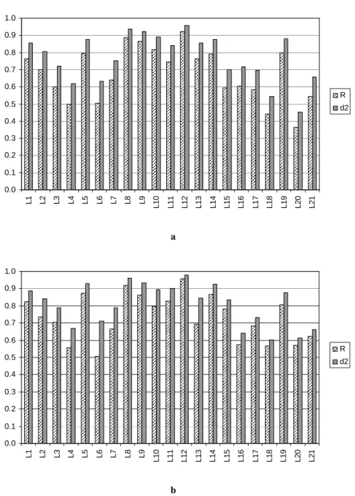
Figure 4.1 Performance indexes of all MLR models in the (a) training and (b) test periods for the Kaiser criterion. ...58
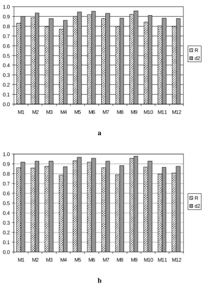
Figure 4.2 Performance indexes of all MLR models in the (a) training and (b) test periods for the ODV90 criterion. ...59
Figure 7.1 Example of the first three steps of SWANN1 methodology (a-c) and
its final result (d) for the case of three input neurons...90
Figure 7.2 Example of the result of five steps of SWANN2 methodology (a-e)
and its final result (f) for the case of three input neurons...91
Figure 7.3 Variation of AIC value in the training set with the increase of the number of IHL synapses in SWANN2 models using OVs as inputs and the
activation function sine. ...93
Figure 7.4 SWANN2 model using OVs as inputs and the activation function
sine. ...94
Figure 7.5 Example of the predictions of: (a) O3 concentrations (with PCs and
Figure 8.2 Procedure to apply GA for defining threshold regression models. .... 103
Figure 9.1 Example of tree representation of expressions used in GP and respective formula. ... 111
Figure 9.2 Example of crossover operation between two trees. ... 112
Figure 9.3 Examples of mutation operation in: (a) a function; and (b) a terminal... 113
Figure 9.4 GP procedure... 114
Figure 9.5 Occurrence (in percentage) of each input for the 4 GP runs in the 20 best solutions of the last generation using 3, 4 and 5 populations (P3, P4 and P5): (a) OV and (b) PC... 117
Figure 9.6 Box and whisker diagrams with the performance indexes of GP models in training (a and b) and test (c and d) periods... 118
Figure 9.7 Performance of the best GP model in all test period... 119
Figure 10.1 Occurrence of each input for the 10 MGP runs in the best solutions (10 individuals) and in the 20 best solutions of the last generation (200 individuals). ... 124
Table 2.1 Site characteristics of the air quality monitoring network of Oporto Metropolitan Area ...15
Table 2.2 Air pollutants whose concentrations are measured at each monitoring site ...16
Table 2.3 Annual averages of SO2 concentrations at each site (it should not
exceed 20 µg m-3 for ecosystem protection) and the correspondent PAD (in brackets) ...17
Table 2.4 Number of exceedances of the limit established by the European Union for the protection of human health regarding daily averages of PM10
concentrations and the correspondent PAD (in brackets) ...18
Table 2.5 Annual averages of PM10 concentrations at each site (it should not
exceed 40 µg m-3 for the protection of human health) and the correspondent PAD (in brackets)...18
Table 2.6 Annual average NO2 concentrations at each site (it should not exceed
40 µg m-3 for the protection of human health) and the correspondent PAD (in brackets) ...19
Table 2.7 Annual average NOx concentrations at each site (it should not exceed
30 µg m-3 for the protection of vegetation) and the correspondent PAD (in brackets) ...19
Table 2.8 Exceedances of the O3 thresholds for public information (180 µg m -3
) established by the European Union and the correspondent PAD (in brackets)...21
Table 2.9 Exceedances of the standard value established by the European Union for human health protection, regarding maximum daily 8-hour average of O3 concentration and the correspondent PAD (in brackets) ...21
Table 2.10 Values of AOT40v at each site (it should not exceed 16.3 µg m -3
h-2 averaged over five years, for the protection of vegetation) and the correspondent PAD (in brackets) ...21
Table 3.1 Main results of the PCA application for the analysed pollutants at all sites...26
during the third quarter of 2004... 52
Table 4.2 Number of PCs selected for each analysed period using the two criteria: Kaiser (left) and ODV90 criterion (right)... 53
Table 4.3 Relative frequency (in percentage) of each pair of monitoring sites with important contributions in the same PC during the first two years of study (eight periods) using Kaiser criterion (upper triangular matrix) and ODV90
criterion (lower triangular matrix)... 55
Table 4.4 MLR models used to estimate the air pollutant concentrations at all removed monitoring sites using the values measured at other sites in Oporto-MA for the Kaiser criterion ... 56
Table 4.5 MLR models used to estimate the air pollutant concentrations at all removed monitoring sites using the values measured at other sites in Oporto-MA for ODV90 criterion ... 56
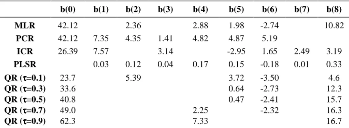
Table 6.1 Regression parameters for all statistical models for O3 concentrations
prediction... 78
Table 6.2 Regression parameters for all statistical models for PM10
concentrations prediction... 79
Table 6.3 Varimax rotated factor loadings ... 79
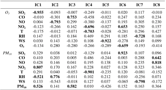
Table 6.4 Correlation matrix between the original variables and the IC for O3
and PM10... 80
Table 6.5 Performance indexes of the different statistical models for the training period ... 82
Table 6.6 Performance indexes of the different statistical models for the test period... 82
Table 7.1 Number of IHL synapses, hidden neurons and parameters presented by SWANN1 and SWANN2 models obtained for the different activation
functions and type of input variables... 95
Table 7.2 Performance indexes of the SWANN1 and SWANN2 models in the
training set for predicting O3 and PM10 concentrations ... 95
Table 7.3 Performance indexes of the SWANN1 and SWANN2 models in the
Table 8.1 Statistically significant regression parameters for TR-GA (M1 to M6) and MLR models and correspondent RMSE value in the training data ...105
Table 8.2 Performance indexes of the TR-GA and MLR models in the test period...105
Table 9.1 Values of GP control parameters...115
Table 9.2 Principal components varimax rotated loadings ...116
Table 10.1 Best solutions of the 10 MGP runs and correspondent RMSE in the training period ...125
Table 10.2 Performance indexes of the best solutions of the 10 MGP runs in the test period ...126
List of Abbreviations
AIC Akaike Information Criterion
AN Antas
ANN Artificial neural network
AOT40 Accumulated exposure over a threshold of 40 ppb AOT40v Averaged exposure Over a Threshold of 40 ppb
AQMN Air quality monitoring network
BG Baguim BV Boavista CA Cluster analysis CL Cluster CS Custóias E East EC European Council ER Ermesinde EU European Union GA Genetic algorithm GP Genetic programming
HOL Hidden-to-output layer
IC Independent component
ICA Independent component analysis
ICi Independent component i
ICR Independent component regression
IHL Input-to-hidden layer
k-NN k-nearest neighbours
LB Leça do Balio
MAE Mean absolute error
MLR Multiple linear regression
MT Matosinhos
N North
NE Northeast
NW Northwest
ODV90 90% of the original data variance
Oporto-MA Oporto Metropolitan Area
OV Original variable
PAD Percentage of available data
PC Principal component
PCA Principal component analysis
PCi ith principal component
PCR Principal component regression
PLSR Partial least squares regression
PM Particulate matter PR Perafita Qi i th annual quarter QR Quantile regression RH Relative humidity
RMSE Root mean squared error
S South
SE Southeast
SH Senhora da Hora
sig Sigmoid function
sin Sine function
SR Solar radiation
SSE Sum of the squared errors
T Air temperature
tgh Hyperbolic tangent function
TR Threshold regression
USEPA United States Environmental Protection Agency
UV Ultraviolet
VC Vila do Conde
VOC Volatile Organic Compounds
VR Vermoim
VT Vila Nova da Telha
W West
WBG World Bank Group
WHO World Health Organization
α Significance level i αˆ Regression parameters i βˆ Regression parameters i νˆ Regression parameters
ε Error associated with the regression
λ Eigenvalue
θ Bias
σ
ˆ Standard deviationσ2 Variance
τ Percentile
(X)-1 Inverse of the matrix X
(X)T Transpose of the matrix X |X| Determinant of the matrix X
B Regression parameters matrix
b Regression parameters vector
bjp Loading of the original variable j in the principal component p BPLS Regression parameters of partial least squares regression
c y weight vector
C y weights matrix
Cov Covariance matrix
CO Carbon monoxide
d Index of threshold variable
d2 Index of agreement of second order F() Cumulative probability density function
I Identity matrix
k Number of parameters
n Number of data points
NO Nitrogen oxide
NO2 Nitrogen dioxide
NOx Nitrogen oxides
O3 Tropospheric ozone
O3|t+24h Next day hourly average ozone concentrations
P X loadings matrix
p X loadings vector
PM10 Particulate matter with aerodynamic diameter smaller than 10 µm
PM2.5 Particulate matter with aerodynamic diameter smaller than 2.5 µm
R Pearson correlation coefficient
r Threshold value
SO2 Sulphur dioxide
Sxxi Sum of squares related to xi
t Student t distribution T X score matrix t X score vector U y score matrix u y score vector W X weight matrix w X weight vector wi Weight value
X Matrix of the explanatory variables
X0 X standardized matrix
xd Threshold variable
i
Yˆ Model output
i
Y Average of the output variable
y Output value
y Vector of the dependent variable
Chapter 1
1.
Introduction
This chapter describes the project associated with this thesis. The importance of this study is also demonstrated. At the end, there is a description of the structure of the thesis.
1.1. Scientific relevance
Clean air is considered to be a basic requirement of human health. The quality of the air is the result of a complex interaction of many factors that involve the chemistry and motions of the atmosphere, as well as the emissions of a variety of pollutants from sources that are both natural and anthropogenic.
Before the increase of large cities and industries, the nature was able to keep the air fairly clean. Wind mixed and dispersed the gases, rain washed the dust and other easily dissolved substances to the ground and plants absorbed carbon dioxide and replaced it by oxygen. With urbanisation and industrialisation, humans started to release more wastes into the atmosphere than nature could manage with. Thus, these concentrated gases exceed safe limits and became a pollution problem.
Air pollution can not be considered a local problem. The air pollutants released in one country can be transported by the wind, causing several negative impacts (in human health, vegetation, ecosystems, climate and materials) elsewhere. Thus, air pollution should be considered as a transboundary concern.
European Union established several directives related with air quality. These directives established limit values for air pollutant concentrations concerning the protection of the human health, vegetation and ecosystems. They also indicate the number of monitoring sites that should operate according to population size and pollution levels. However, the number and location of the monitoring sites should be optimized for the different regions. In other words, the redundant measurements should be avoided due to the high cost of the monitoring equipment maintenance.
One of the most important air pollutant usually associated with poor air quality is tropospheric ozone (O3). O3 is naturally present in the atmosphere, but in elevated
amounts it is damaging to the living tissue of plants and animals. However, the most relevant pollutant for air quality is particulate matter (PM). An important target of this thesis is the prediction of concentrations of O3 and PM10 (particulate
matter with aerodynamic diameter smaller than 10 µm) with a day in advance. Thus, the persons belonging to risk groups (with respiratory problems, children and elderly) can be advised for high concentrations episodes. Other components important in air quality include carbon monoxide, sulphur dioxide, NOx and VOC
(O3 precursors), and air toxics such as benzene, mercury and other hazardous air
pollutants.
The need for improved understanding of the science of air quality remains a priority for the wider scientific and user communities. Despite improvements in technology, users still require new, robust management and assessment tools to formulate effective control policies and strategies for reducing the health impact of air pollution. Accordingly, this thesis presents statistical methods useful for policy makers seeking to improve air quality management in their cities.
1.2. Thesis structure
The project associated with this document, entitled Development and Application of Statistical Methods to Support Air Quality Policy Decisions, was performed at
Departamento de Engenharia Química of Faculdade de Engenharia da Universidade do Porto from 2006 to 2009.
The thesis was divided in two parts: (i) management of air quality monitoring networks (Part I); and (ii) prediction of air pollutant concentrations (Part II). Part I contains the Chapters 2 to 4, while Part II contains the Chapters 5 to 10.
Chapter 2 describes the air pollutants whose monitoring is of particular interest for the characterization of the air quality. Their sources, effects and legislation related with their concentrations are the main topics focused. Additionally, this chapter: (i) characterizes the region where the air quality was measured; (ii) refers the equipment used for each air pollutant monitoring; and (iii) determines for a specific period the number of exceedances to the limits established by the EU for protection of human health, vegetation and ecosystems.
Chapter 3 shows how principal component analysis and cluster analysis can be applied to define the number of monitoring sites that should operate in an air quality monitoring network (AQMN). Additionally, the location of the main emission sources was identified based on the influence of wind direction on the increase of the air pollutant concentrations.
In Chapter 4, principal component analysis was applied using another criterion to select the number of principal components. This number, corresponding to the minimum number of monitoring sites that should operate, was then compared with the value presented by the European legislation. At the end of this chapter, the air pollutant concentrations at the removed monitoring sites were estimated using the values of the selected monitoring sites.
Chapter 5 presents several previous studies about prediction of O3 and PM10
concentrations through statistical models.
Chapter 6 shows the comparison of the performance of five linear models in the prediction of O3 and PM10 concentrations.
Chapter 7 presents two step-by-step methodologies to define artificial neural network models. These models were applied to predict the concentrations of the same air pollutants.
Chapter 8 shows how to apply genetic algorithms to define threshold regression models for prediction of O3 concentrations.
In Chapter 9, genetic programming was applied to predict O3 concentrations.
In Chapter 10, multi-gene genetic programming was applied to predict PM10
concentrations.
Finally, Chapter 11 presented the main conclusions of this thesis and some suggestions for future work.
Part I
(from www.qualar.org)
Management of Air Quality Monitoring Networks
Boavista monitoring siteChapter 2
2.
Air Quality Evaluation in Oporto Metropolitan Area
This chapter describes the air pollutants whose monitoring is of particular interest for the characterization of the air quality. Their sources, effects and the legislation related with their concentrations are the main topics of this chapter. Additionally, the aims are: (i) characterize the region where the air quality was measured; (ii) refer to the equipment used for each air pollutant monitoring; and (iii) determine for this period the number of exceedances to the limits established by the European Union for protection of human health, vegetation and ecosystems.
The contents of this chapter were adapted from: (i) Pires, J.C.M., Sousa, S.I.V., Pereira, M.C., Alvim-Ferraz, M.C.M., Martins, F.G., 2008. Management of Air Quality Monitoring using Principal Component and Cluster Analysis – Part I: SO2 and PM10. Atmospheric
Environment 42 (6), 1249-1260; and (ii) Pires, J.C.M., Sousa, S.I.V., Pereira, M.C.,
Alvim-Ferraz, M.C.M., Martins, F.G., 2008. Management of Air Quality Monitoring using Principal Component and Cluster Analysis – Part II: CO, NO2 and O3. Atmospheric
Environment 42 (6), 1261-1274.
2.1. Sulphur dioxide
Sulphur dioxide (SO2) is one of the most important pollutants, as it results from
the combustion of sulphur compounds. Volcanoes and oceans are the major natural sources of SO2 (Carmichael et al., 2002; Garg et al., 2006; Reddy and
Venkataraman, 2002; World Health Organization - WHO, 2000). Anthropogenic emissions of SO2 come from the combustion of fossil fuels (mainly coal and heavy
oils), biomass burning and the smelting of sulphur containing ores.
Many efforts have been done to reduce SO2 emissions; consequently, in the last 20
Western industrialized countries (Nunnari et al., 2004). SO2 and its oxidation
by-products are removed from the atmosphere by wet and dry deposition (acid precipitation). Besides these transformation and removal processes, SO2 can be
carried out over large distances, causing transboundary pollution (ApSimon and Warren, 1996).
SO2 is an irritant gas when inhaled and at high concentrations may cause breathing
difficulties in people directly exposed to it. Absorption of SO2 in the nose mucous
membranes and in the upper respiratory tract results from its solubility in water (WHO, 2000). The effects of SO2 inhalation appear in only a few minutes and
people suffering from asthma and chronic lung disease may be especially susceptible to its adverse effects. This pollutant also affects plants and depending on its concentration levels, can produce: chlorophyll degradation; reduction of photosynthesis; raise of respiration rates; and changes in protein metabolism (Carlson, 1979; Lee et al., 1997). Nevertheless, sulphur is an important nutrient for plants due to the fact that, by instance, atmospheric sulphur may be taken up by leaves of some species, contributing to the plant vitality in soils with low sulphur concentrations such as calcareous soils. SO2 (combined with other air pollutants
and under specific conditions of relative humidity, temperature and precipitation) is responsible for the deterioration of materials, such as metals and stones. In many parts of Europe, some monuments which resisted deterioration for hundreds or even thousands of years have shown an accelerated degradation of their surface in the last decades.
The European Union (EU) established limit values for SO2 concentrations: (i) the
hourly limit for the protection of human health (350 µg m-3, not to be exceeded more than 24 times per year); (ii) the daily limit for the protection of human health (125 µg m-3, not to be exceeded more than 3 times per year); and (iii) the annual limit for protection of ecosystems (20 µg m-3) (EC Directive, 1999).
2.2. Particulate matter
Particulate matter (PM) is the designation of solid and liquid particles suspended in the atmosphere. They are emitted by both, natural (volcanic eruptions, seismic activity and forest fires) and anthropogenic sources (all types of man-made combustion and some industrial processes).
PM is one of the most important air pollutants that adversely influence human health in Europe (Koelemeijer et al., 2006). In the last decade, several studies were published about the impact of PM on human health (Alvim-Ferraz et al., 2005; Brunekreef and Holgate, 2002; Dockery and Pope, 1994; Hoek et al., 2002). Long exposure to PM10 and to PM2.5 (particles with an aerodynamic diameter smaller
than 10 and 2.5 µm, respectively) has been associated with respiratory and cardiovascular diseases. Recent research seems to indicate that PM10 are
associated with childhood morbidity and mortality (Kappos et al., 2004).
Aiming the protection of human health, the EU established two limits for PM10,
which should be enforced on two different periods of time; the first beginning in 2005 and the last one in 2010. The limits to be enforced from 2005 until 2010 are: (i) the daily limit of 50 µg m-3, not to be exceeded more than 35 times per year; and (ii) the annual limit of 40 µg m-3. The limits to be enforced from 2010 are: (i) the daily limit of 50 µg m-3, not to be exceeded more than 7 times per year; and (ii) the annual limit of 20 µg m-3 (EC Directive, 1999).
2.3. Carbon monoxide
Carbon monoxide (CO) is a colourless, practically odourless, tasteless and no irritating gas which is the result of the incomplete oxidation of carbon in combustion (Raub, 1999; Raub et al., 2000). The main sources are the combustion of fuel (that occurs when the ratio air-to-fuel presents low values), industrial emissions and other combustion sources (as coal, gas, wood and kerosene). Natural sources, such as volcanoes, natural gases in coal mines and forest fires, have also an important contribution. The emissions of CO increase significantly
during the cold weather. In these conditions, the engines need more fuel to work and some emission control devices, such as oxygen sensors and catalytic converters, operate less efficiently when they are cold (Raub et al., 2000; United States Environmental Protection Agency - USEPA, 2004).
The effects in the human health associated to the presence of CO depend on its concentration and the duration of exposure. At low concentrations, CO causes fatigue in healthy people and chest pain in people with heart disease. At high concentrations, it causes headaches, confusion and nausea. When inhaled, CO is absorbed from the lungs to the bloodstream, where it forms a complex with haemoglobin known carboxyhaemoglobin. The presence of this complex reduces the oxygen carrying capacity, causing hypoxia (low oxygen level available to the body tissues) (Raub, 1999; Raub et al., 2000; USEPA, 2000; USEPA, 2004; WHO, 2000). CO is one of the contaminants found normally in the atmosphere that requires prevention and control measures to ensure adequate protection of the human health.
EU established 10 mg m-3 as a limit value for the protection of human health (EC Directive, 2000) based in the maximum daily 8-hour average concentration.
2.4. Nitrogen oxides
Nitrogen oxides (NOx) are a group of highly reactive gases. These gases contain
atoms of nitrogen and oxygen in different proportions. Nitrogen oxide (NO) and nitrogen dioxide (NO2) are the most important gases of this group and they are
considered significant pollutants in the troposphere (USEPA, 1998; World Bank Group - WBG, 1998). Anthropogenic emissions of NOx result from the
combustion processes, including motor vehicles, electric utilities, and other industrial, commercial and residential sources that burn fossil fuels. Natural events, such as anaerobic biological processes in soil and water, volcanic activity and photochemical destruction of nitrogen compounds in the upper atmosphere, have also a high contribution for NOx emissions (USEPA, 1998; WBG, 1998).
Nitrogen oxides have diverse negative effects (Hashim et al., 2004; Kalabokas et al., 2002; USEPA, 1998; WBG, 1998; WHO, 2000), such as: (i) formation of acid rain – they react with other substances in the air to form acids which fall to earth as rain, fog, snow, or dry particles; (ii) deterioration of the water quality - increased nitrogen loading in water bodies, particularly coastal estuaries, upsets
the chemical balance of nutrients used by aquatic plants and animals; (iii) formation of toxic chemicals – NOx reacts with common organic chemicals to
form a wide variety of toxic products, such as nitrate radicals, nitroarenes and nitrosamines; (iv) reduction of the visibility – nitrogen dioxide can block the transmission of light; (v) contribution to the increase of the earth’s temperature – one of the nitrogen oxides, nitrous oxide, is a greenhouse gas; and (vi) formation of ground-level ozone – in the presence of hydrocarbons and sunlight, NOx
contribute to the formation of tropospheric ozone, which can cause serious respiratory problems.
EU established limit values for NO2 and NOx (EC Directive, 1999). Concerning
hourly average concentrations, NO2 limit for the protection of human health is 200
µg m-3 and may not be exceed more than 18 times in the year (limit value to be met till January of 2010). Concerning annual average concentrations, NO2 limit for
the protection of human health is 40 µg m-3 (limit value to be met till January of 2010) and NOx limit for protection of the vegetation is 30 µg m
-3
.
2.5. Ozone
Ozone (O3) is a strong photochemical oxidant found in the troposphere and in
other layers of the atmosphere. While ozone has an important role in the stratosphere (protection from the ultraviolet radiation), in the troposphere this irritating and reactive molecule has negative impacts on human health, climate, vegetation and materials (Alvim-Ferraz et al., 2006; Chan et al., 1998). Concerning human health effects, the most important are: (i) damage to respiratory tract tissues; (ii) death of lung cells and increased rates of cell replication
(hyperplasia); (iii) inflammation of airways; and (iv) increase of the respiratory symptoms, such as cough, chest soreness, difficulty in taking a deep breath and, in some cases, headaches or nausea (Kley et al., 1999; Leeuw, 2000). Concerning climate, a temperature increase is expected to be related to the tropospheric ozone increase, because it is a greenhouse gas and influences the atmospheric residence time of other greenhouse gases (Bytnerowicz et al., 2006). In vegetation, it causes leaf injury, growth and yield reduction, and changes in the sensitivity to biotic and abiotic stresses (Alvim-Ferraz et al., 2006; Leeuw, 2000). Concerning materials, ozone in combination with other atmosphere pollutants contributes to the increase of the corrosion on building materials like steel, zinc, copper, aluminium and bronze (Leeuw, 2000).
The presence of ozone in the troposphere is a result of three basic processes: (i) photochemical production by the interaction of hydrocarbons and nitrogen oxides (emitted by gasoline vapours, fossil fuel power plants, refineries, and other industries) under the action of suitable ambient meteorological conditions (Guerra et al., 2004; Strand and Hov, 1996; Zolghadri et al., 2004); (ii) tropospheric/stratospheric exchange that causes the transport of stratospheric air, rich in ozone, into the troposphere (Dueñas et al., 2002); and (iii) horizontal transport due to the wind that brings ozone produced in other regions.
EU established limit values for ozone in the ambient air (EC Directive, 2002). The information threshold (considered to carry health risks for short-time exposure of groups particularly sensible) is 180 µg m-3 for hourly average concentration, and the alert threshold (considered to carry health risks for short-time exposure of the population in general) is 240 µg m-3. The O3 target value for the protection of the
human health is 120 µg m-3 concerning maximum daily 8-hour average concentrations and may not be exceeded more than 25 days per calendar year averaged over three years (limit value to be met till 2010). Concerning the cumulative ozone exposure index (AOT40 – Accumulated exposure Over a Threshold of 40 ppb or 80 µg m-3) calculated from 1 h values from May to July,
the O3 target value for the protection of the vegetation is 18000 µg m -3
h-1 averaged over five years (limit value to be met till 2010). The long-term objectives for O3 in
Europe are: (i) maximum daily 8-hour average of 120 µg m-3 for the protection of the human health; and (ii) AOT40 calculated from 1 h values from May to July of 6000 µg m-3 h-1.
2.6. Air quality data
Oporto is the second largest city of Portugal, located at North. The important air pollution sources in Oporto Metropolitan Area (Oporto-MA) are vehicle traffic, an oil refinery, a petrochemical complex, a thermoelectric plant (planned for working with natural gas), an incineration unit and an international shipping port (Pereira et al., 2007).
The air quality data was collected from the monitoring sites integrated in the air quality monitoring network (AQMN) of Oporto-MA, managed by the Regional Commission of Coordination and Development of Northern Portugal (Comissão de Coordenação e Desenvolvimento Regional do Norte), under the responsibility
of the Ministry of Environment. The AQMN of Oporto-MA is currently composed of 14 monitoring sites that regularly monitor the air levels of SO2, PM10, CO, NO,
NO2, NOx and O3. PM2.5, benzene, toluene and xylene are also measured in some
monitoring sites of the network.
SO2 concentrations were obtained by the ultraviolet fluorescence method,
according to the EC Directive 1999/30/EC (EC Directive, 1999) using the AF21M equipment from Environment SA (Pereira et al., 2007). PM10 concentrations were
obtained through the beta radiation attenuation method, considered equivalent to the method advised by the EU Directive 1999/30/EC (EC Directive, 1999), using the MPSI 100 I et E equipment from Environment SA (Pereira et al., 2005). Nondispersive infrared spectrometric method was applied to measure the CO concentrations (Sousa et al., 2006), according to the EU Directive 2000/69/EC (EC Directive, 2000). NO2 and NOx were obtained through the chemiluminescence
method (Sousa et al., 2006), according to EU Directive 1999/30/EC (EC Directive, 1999). Ozone measurements, according to EU Directive 2002/3/EC (EC Directive, 2002), were performed through UV-absorption photometry using the equipment 41 M UV Photometric Ozone Analyser from Environment S.A. (Pereira et al., 2005). This equipment was submitted to a rigid maintenance program, being calibrated each 4 weeks. Measurements were continuously registered and hourly average concentrations (in µg m-3) were recorded.
2.7. Exceedances to EU limits
The exceedances to the limits established by the EU were evaluated for the period between 2003 and 2005. Two of the fourteen monitoring sites that constitute the AQMN of Oporto-MA showed high percentage of missing data during the analysed period. The exceedances to EU limits were not evaluated in these monitoring sites. The monitoring sites selected for this study were: Antas (AN), Baguim (BG), Boavista (BV), Custóias (CS), Ermesinde (ER), Leça do Balio
(LB), Matosinhos (MT), Perafita (PR), Senhora da Hora (SH), Vermoim (VR), Vila do Conde (VC) and Vila Nova da Telha (VT). Table 2.1 shows the main
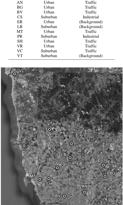
AQMN monitoring site characteristics, including the type and the main pollution sources associated to them (QualAr, 2006). Figure 2.1 presents the map of Oporto-MA with the locations of these monitoring sites. Table 2.2 shows, from the five air pollutants described above, the ones whose concentrations are measured at each monitoring site. The ER site presented high percentage of missing PM10 data.
Thus, the exceedances to EU limits for PM10 were not evaluated at ER site.
The analysis of SO2 data showed that their concentrations were in compliance at
all sites with the legislation established by the EU for the protection of human health (EC Directive, 1999). The hourly limit was exceeded in four monitoring sites: (i) CS (once in 2004); (ii) MT (4, 3 and 2 times in 2003, 2004 and 2005, respectively); (iii) PR (15 times in 2003); and (iv) VT (once in 2004).
Table 2.1 Site characteristics of the air quality monitoring network of Oporto Metropolitan
Area
Site Type Main pollution source
AN Urban Traffic BG Urban Traffic BV Urban Traffic CS Suburban Industrial ER Urban (Background) LB Suburban (Background) MT Urban Traffic PR Suburban Industrial SH Urban Traffic VR Urban Traffic VC Suburban Traffic VT Suburban (Background)
Figure 2.1 Location of the monitoring sites in the map of Oporto-MA (from Google
Table 2.2 Air pollutants whose concentrations are measured at each monitoring site Site SO2 PM10 CO NO2 O3 AN × × × × BG × × × BV × × × × × CS × × × × × ER × × × × LB × × × × × MT × × × × × PR × × × × × SH × × × × VR × × × × × VC × × × × × VT × × × × ×
According to the referred legislation, the SO2 hourly average concentrations limit
of 350 µg m-3 cannot be exceeded more than 24 times a year (~0.3% of the total number of hours) in order to be in compliance with the norm (EC Directive, 1999). The PR and MT sites showed the larger number of exceedances during the analysed period. It is noted that all of the exceedances for the PR site occurred in 2003, which represent ~0.2% of the available hourly average concentrations and that the correspondent percentages for MT site were even lower (~0.05%). The daily average concentrations of SO2 were calculated when more than 75% of the
hourly average concentrations were available. The daily limit of SO2
concentrations is 125 µg m-3 and cannot be exceeded more than 3 times a year (~0.8% of the total number of days) to be in compliance with the norm (EC Directive, 1999). The daily limit was exceeded only once at the PR site, representing ~0.3% of the available daily average concentrations. To determine these exceedances (to hourly and daily limits), the minimum for the percentage of available data (PAD) was 73%.
Table 2.3 shows the annual averages of SO2 concentrations calculated at each
monitoring site for the years 2003, 2004 and 2005 as well as the correspondent PAD. It is observed that those annual averages did not change considerably during the analysed period. MT site showed the highest annual average values
Table 2.3 Annual averages of SO2 concentrations at each site (it should not exceed 20 µg m-3 for ecosystem protection) and the correspondent PAD (in brackets)
Year BV CS ER LB MT PR SH VR VC VT 2003 6.5 (97) 5.8 (91) 4.5 (97) 6.0 (99) 11.1 (98) 6.9 (96) 6.4 (97) 4.6 (96) 2.5 (98) 5.0 (85) 2004 5.5 (98) 6.8 (99) 5.3 (100) 6.6 (100) 10.3 (100) 5.1 (95) 8.9 (99) 4.3 (99) 2.7 (99) 3.9 (98) 2005 5.7 (100) 7.5 (99) 5.8 (73) 5.7 (90) 9.5 (100) 4.9 (99) 9.5 (100) 5.5 (91) 3.1 (99) 2.8 (100)
due to the proximity of one emission source; nevertheless, even there, the annual average concentrations were about half of the 20 µg m-3 limit established for ecosystem protection by the EC Directive (1999).
Table 2.4 presents the number of exceedances of the limit of 50 µg m-3 established by the EU for the protection of human health and the correspondent PAD, regarding the daily average concentrations of PM10. In order to be in compliance,
the limit cannot be exceeded more than 35 times a year which corresponds to ~10% of the total number of available days (EC Directive, 1999). The number of exceedances allowed by the EU was surpassed at all monitoring sites during the analysed years. VC site showed the highest number of exceedances, representing about approximately half of the available data. Table 2.5 shows the annual averages of PM10 concentrations at each monitoring site and the correspondent
PAD. During the entire studied period, only the VT monitoring site was in compliance of the annual limit of 40 µg m-3 implemented by the EC Directive (1999) for the protection of human health. Besides the traffic and industrial emissions of PM10, the regional transport played an important role in the pollutant
concentration. The research made by Pereira et al. (2005) showed that even at rural sites (absence of direct influence of emission sources) exceedances were observed due to intra-regional pollutant transport.
Table 2.4 Number of exceedances of the limit established by the European Union for the
protection of human health regarding daily averages of PM10 concentrations and the correspondent PAD (in brackets)
Year AN BV CS LB MT PR SH VR VC VT 2003 127 (93) 111 (98) 86 (88) 114 (82) 92 (92) 123 (97) 121 (85) 107 (89) 167 (95) 62 (73) 2004 92 (90) 135 (95) 107 (96) 82 (98) 104 (98) 78 (95) 79 (98) 59 (72) 160 (89) 72 (98) 2005 86 (95) 115 (100) 134 (92) 67 (83) 122 (99) 80 (96) 104 (94) 88 (85) 161 (99) 86 (100)
Table 2.5 Annual averages of PM10 concentrations at each site (it should not exceed 40 µg m-3 for the protection of human health) and the correspondent PAD (in brackets)
Year AN BV CS LB MT PR SH VR VC VT 2003 46.2 (95) 43.2 (98) 36.4 (90) 45.6 (84) 40.0 (93) 45.2 (97) 47.0 (87) 41.6 (92) 53.2 (96) 37.1 (74) 2004 40.9 (92) 50.2 (94) 40.5 (98) 34.9 (98) 41.9 (98) 39.5 (96) 37.3 (99) 36.3 (75) 52.7 (90) 35.7 (98) 2005 40.9 (95) 44.4 (99) 48.2 (93) 35.2 (84) 44.9 (98) 38.3 (97) 42.4 (95) 40.7 (87) 51.2 (98) 38.8 (99)
During the analysed period, the maximum daily 8-hour average concentrations of CO did not exceed the limits established by the EU for the protection of human health (10 mg m-3) (EC Directive, 2000) at any monitoring site.
According to the legislation established by EU for the protection of human health, the hourly average concentration of NO2 may not be exceed 200 µg m
-3
more than 18 times a year (EC Directive, 1999). The LB site presented the highest number of exceedances (20 hourly average concentrations) that occurred only in 2005. This means that the number of exceedances allowed by the EU (18 exceedances in a year) was surpassed at this site. As the annual average NO2 concentration at this
site was not usually high, these exceedances were probably due to industrial emissions. The exceedances of hourly limit occurred also 13 times at MT site
(2005), 6 times at VR site (2004), 4 times at AN and BV sites (2005) and twice at BG site (2005). To determine these exceedances, the minimum for the percentage of available data (PAD) was 63%. Table 2.6 shows the annual average of NO2
concentrations calculated at each monitoring site for the years of 2003, 2004 and 2005 as well as the correspondent PAD. AN, BV and MT were the sites that presented annual average concentrations above the limit established by the EU for the protection of human health (40 µg m-3) (EC Directive, 1999). Besides the influence of industrial sources, these sites are strongly influenced by the traffic emissions. Table 2.7 shows the annual average of NOx concentrations calculated at
each monitoring site and the correspondent PAD. The annual limit for the protection of vegetation (30 µg m-3) was exceeded at all sites with exception
Table 2.6 Annual average NO2 concentrations at each site (it should not exceed 40 µg m -3 for the protection of human health) and the correspondent PAD (in brackets)
Year AN BG BV CS ER LB MT PR SH VR VC VT 2003 43.4 (94) 34.9 (95) 48.9 (90) 27.3 (86) 28.6 (96) 27.8 (97) 43.8 (99) 21.6 (93) 32.8 (93) 31.4 (93) 29.3 (98) 21.4 (95) 2004 45.4 (93) 30.5 (93) 39.7 (63) 27.6 (96) 30.0 (100) 26.1 (99) 41.3 (99) 18.4 (98) 36.4 (99) 32.5 (96) 23.8 (81) 18.5 (98) 2005 48.3 (94) 31.6 (100) 42.6 (98) 29.0 (99) 29.8 (94) 27.5 (86) 41.0 (95) 19.9 (95) 35.5 (99) 32.3 (89) 22.3 (80) 17.9 (95)
Table 2.7 Annual average NOx concentrations at each site (it should not exceed 30 µg m -3 for the protection of vegetation) and the correspondent PAD (in brackets)
Year AN BG BV CS ER LB MT PR SH VR VC VT 2003 96.4 (94) 68.5 (95) 114.5 (90) 44.1 (86) 49.2 (96) 52.1 (98) 98.3 (99) 31.3 (93) 67.0 (93) 58.4 (93) 70.1 (98) 21.4 (95) 2004 110.5 (93) 63.1 (93) 101.6 (63) 46.9 (96) 49.5 (100) 52.9 (99) 91.1 (99) 30.3 (98) 63.3 (99) 58.3 (96) 63.7 (81) 28.7 (98) 2005 104.5 (94) 62.8 (100) 86.4 (98) 48.3 (99) 45.8 (94) 49.4 (86) 84.2 (95) 28.9 (95) 61.0 (99) 55.4 (89) 61.7 (80) 26.3 (95)
of VT site (during the entire period) and PR site (in 2005) (EC Directive, 1999). As it happened with NO2, AN, BV and MT sites presented the highest annual
average concentrations of NOx. For both pollutants, there was not a significant
variation of their annual average concentration during the analysed period.
Table 2.8 presents the exceedances of the O3 thresholds for public information
(180 µg m-3) established by the EU and the correspondent PAD (EC Directive, 2002). The AN, BG, ER, LB, VR and VT sites presented the highest numbers of exceedances during the entire analysed period. The threshold for public alert (240
µg m-3) was exceeded once at BG, VR and VT sites in 2003. Table 2.9 presents the exceedances of the standard value established by the EU for the protection of human health and the correspondent PAD, regarding maximum daily 8-hour average of O3 concentration (120 µg m
-3
, that may not be exceeded more than 25 times a year averaged over three years). During the entire analysed period (three years), ER site presented the highest number of exceedances; nevertheless, even there, the maximum number of exceedances allowed by the EU was obeyed. Concerning the protection of vegetation, the value of AOT40 is calculated by the sum of the difference between hourly average concentrations greater than 80 µg m-3 (equal to 40 parts per billion) and 80 µg m-3 over a given period using only the 1 hour values measured between 8 and 20 hours (Central European Time) each day. At all sites, all possible measured data was not available. Therefore, the calculated value of AOT40 was divided by the measured hourly values (AOT40v –
Averaged exposure Over a Threshold of 40 ppb or 80 µg m-3) and compared to the ratio between AOT40 limit and the total possible number of hours (16.3 µg m-3 h-2 averaged over five years). Table 2.10 shows the values of AOT40v calculated at
each monitoring site and the correspondent PAD. During the entire period, the O3
limit AOT40v (16.3 µg m -3
h-2 averaged over five years) for the protection of the vegetation was obeyed at all sites.
Table 2.8 Exceedances of the O3 thresholds for public information (180 µg m-3) established by the European Union and the correspondent PAD (in brackets)
Year AN BG BV CS ER LB MT PR VR VC VT 2003 6 (86) 5 (93) 2 (95) 0 (92) 4 (97) 0 (47) 0 (100) 0 (99) 5 (96) 0 (98) 7 (95) 2004 2 (97) 1 (100) 0 (99) 3 (100) 4 (99) 1 (94) 0 (100) 5 (98) 3 (99) 1 (99) 4 (98) 2005 10 (99) 7 (100) 0 (100) 2 (53) 17 (100) 27 (69) 0 (90) 1 (100) 8 (91) 0 (98) 12 (100)
Table 2.9 Exceedances of the standard value established by the European Union for
human health protection, regarding maximum daily 8-hour average of O3 concentration and the correspondent PAD (in brackets)
Year AN BG BV CS ER LB MT PR VR VC VT 2003 7 (87) 9 (94) 1 (96) 5 (94) 11 (98) 0 (47) 1 (100) 3 (100) 10 (98) 5 (98) 12 (97) 2004 4 (98) 3 (100) 1 (99) 7 (100) 11 (100) 3 (95) 2 (100) 11 (100) 9 (100) 2 (100) 6 (99) 2005 7 (100) 9 (100) 3 (100) 1 (53) 23 (100) 19 (70) 6 (91) 13 (100) 17 (92) 9 (99) 17 (100)
Table 2.10 Values of AOT40v at each site (it should not exceed 16.3 µg m -3
h-2 averaged over five years, for the protection of vegetation) and the correspondent PAD (in brackets)
Year AN BG BV CS ER LB MT PR VR VC VT 2003 3.5 (95) 4.0 (99) 1.8 (100) 5.2 (96) 7.7 (98) - 1.7 (99) 4.5 (99) 6.2 (88) 4.7 (100) 7.6 (95) 2004 3.4 (90) 5.4 (100) 1.4 (96) 7.9 (99) 8.0 (99) 3.5 (82) 2.5 (99) 9.2 (99) 4.6 (100) 4.3 (99) 5.8 (98) 2005 3.4 (100) 5.9 (99) 1.4 (99) 5.0 (75) 8.5 (100) 14.5 (75) 2.8 (69) 6.2 (98) 11.9 (99) 5.2 (99) 8.2 (100) 2.8. Conclusions
The analysis to the exceedances to EU limits showed that Oporto-MA presents lower levels of CO and SO2 concentrations. As it is a region strongly influenced
monitoring sites. For NO2, the concerning monitoring sites were AN, BV, LB and
MT. With higher levels of NOx, the equilibrium chemical reaction evolving NOx
and O3 limits the concentrations of the last one. Despite this fact, the limits relative
to O3 concentrations regarding the protection of human health were surpassed at