RBRH, Porto Alegre, v. 22, e51, 2017
Scientiic/Technical Article
http://dx.doi.org/10.1590/2318-0331.0217160071
Statistical validity of water quality time series in urban watersheds
Validade estatística de séries históricas de qualidade da água em bacias urbanas
Marcelo Coelho1, Cristovão Vicente Scapulatempo Fernandes1, Daniel Henrique Marco Detzel1 and Michael Mannich1
1Universidade Federal do Paraná, Curitiba, PR, Brazil
E-mails: [email protected] (MC), [email protected] (CVSF), [email protected] (DHMD), [email protected] (MM)
Received: December 29, 2016 - Revised: June 01, 2017- Accepted: July 07, 2017
ABSTRACT
The water resources quality continuous monitoring is a complex activity. It generates extensive databases with time series of many variables and monitoring points that require the application of statistical methods for the information extraction. The application of statistical methods for frequency analysis of time series is linked to attending of the basic assumptions of randomness, homogeneity, independence, and stationarity. However, despite its importance, the veriication of these assumptions in water quality literature is unusual. Therefore, the present study tests the Upper Iguaçu basin water quality time series against the mentioned hypotheses. Rejection was observed in 15%, 26%, 51% e 31% for randomness, homogeneity, independence, and stationarity, respectively. The results evidenced the strong relation between monitoring strategy, data assessment and meeting of basic statistical assumptions for the analysis of water quality time series. Even with the existence of possible solutions for addressing those issues, the standard monitoring strategies, with irregular frequencies and lack of representativeness in relation to other periods, beyond commercial, act as an obstacle to their implementation.
Keywords: Homogeneity; Independence; Randomness; Stationarity; Monitoring strategies.
RESUMO
O monitoramento quali-quantitativo de recursos hídricos é uma atividade complexa. Sua continuidade dá origem a extensos bancos de dados contendo séries históricas de diversas variáveis e pontos, que exigem a aplicação de métodos estatísticos para extração de informações. A aplicação de métodos estatísticos para a análise de frequências de séries históricas está vinculada ao atendimento aos pressupostos básicos de aleatoriedade, homogeneidade, independência e estacionariedade. Apesar da importância destes critérios, sua veriicação é incomum em literatura de qualidade de água. Neste artigo, estas hipóteses foram testadas em séries históricas da Bacia do Alto Iguaçu. Observou-se rejeição em 15%, 26%, 51% e 31% das séries testadas para aleatoriedade, homogeneidade, independência e estacionariedade, respectivamente. Os resultados evidenciaram a forte relação entre as estratégias de monitoramento, a forma de abordagem dos dados e o atendimento aos pressupostos básicos para análise de séries de qualidade da água. Apesar da existência de possibilidades para solução do problema de não atendimento, as estratégias típicas de monitoramento com frequências irregulares e pouca representatividade em relação a outros períodos, além do horário comercial, representam um obstáculo para sua implementação.
INTRODUCTION
Qualitative monitoring of water resources is a complex activity. It requires the development, constant maintenance and updating of strategies for obtaining representative data and consistent information for the management of water resources. Continuity of monitoring gives rise to extensive databases containing time series of various variables and monitoring points. The analysis of these data requires the application of appropriate statistical methods, especially in urban basins, where processes that alter water quality are diverse and produce high variability.
The application of statistical methods for the analysis of frequencies in time series depends fundamentally on the statistical validity of the series, which is linked to the basic assumptions of randomness, homogeneity, independence and stationarity
(CHADEE; SHARMA, 2003; MERZ; THIEKEN, 2005;
NAGHETTINI; PINTO, 2007; HULLEY; CLARKE; WATT,
2015). In hydrological studies, the veriication of these hypotheses is frequently recommended, however, in water quality literature references that have some recommendation or veriication are rare.
Water quality time series are used in trend analysis (COSTA; OLIVEIRA; SOUZA, 2011; DAHM et al., 2014),
multivariate statistical analyses (WANG et al., 2013; TORRES;
LEMOS; MAGALHÃES JUNIOR, 2016), analysis of variances
(GONÇALVES et al., 2011), mathematical modeling (KONDAGESKI;
FERNANDES, 2009; KNAPIK et al., 2013; VIEIRA et al., 2013),
duration curves (MARIN et al., 2007; FORMIGONI et al., 2011),
linear regression analysis (HIRSCH; MOYER; ARCHFIELD, 2010), among other analyses, however, typically, without prior veriication of the assumptions for analysis.
Costa, Oliveira and Souza (2011) analyzed the presence of trends in time series of annual averages of water quality data in the Upper Iguaçu Basin. The annual averages were used as a solution to the problem of dependence and seasonality in the series. However, no veriication of compliance with the basic assumptions for frequency analysis in time series was performed, and therefore there is no guarantee that the annual averages are statistically representative.
The concepts regarding the assumptions are clearly deined in hydrological studies. Randomness is observed when luctuations of values have natural causes, such as river lows when not inluenced by the presence of a dam. Independence is observed when previous observations do not inluence the next observations in a chronological sequence. A homogeneous time series is observed when all the data comes from a single population. Different populations can be generated in the same series by the inluence of phenomena such as El Niño or seasonality. Finally, a series is said to be stationary when there is no changing of population parameters, such as mean and standard deviation,
over time (NAGHETTINI; PINTO, 2007).
In water quality studies there is no clear and appropriate definition of these concepts to explain cause and effect relationships. This absence is equivalent to considering the series random, independent, homogeneous and stationary, but without proper justiication. Environmental data are susceptible to the presence of non-randomness, dependence, non-homogeneity, and non-stationarity, due to seasonality, the occurrence of extreme
events, urbanization, among other factors. Hence, the need for a more cautious analysis, especially in urban basins, is evident.
The negligent application of traditional statistical methods in series with these characteristics produces unreliable information on parameters and their associated uncertainties, that is, on conidence intervals, p-values, standard deviation, among others
(GILBERT, 1987; HELSEL; HIRSCH, 2002; MCBRIDE, 2005).
In this paper, a veriication of the basic statistical assumptions for frequency analysis in water quality time series of the Upper Iguaçu Basin is performed. These series represent the technical basis of several relevant studies for the management of water resources. The results are accompanied by a critical analysis of the application to water quality data, the discussion of causes and effects of non-attendance, and recommendations on the development of monitoring strategies and approaches to the observed series.
MATERIAL AND METHODS
The research was developed from a database consolidated between 2005 and 2011 for research projects in the Upper Iguaçu Basin and complemented with ive monitoring campaigns in 2012. The time series were submitted to veriication of the attendance to the assumptions for the analysis of frequencies by the application of statistical methods, testing the hypotheses of randomness, homogeneity, independence, and stationarity.
Prior to the veriication of compliance with the basic assumptions, characteristics of the time series, such as sample size, variability, sampling frequencies and seasonality, were analyzed.
Study area
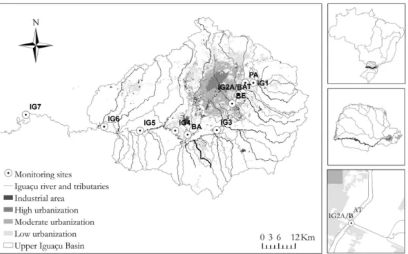
The Upper Iguaçu Basin (Figure 1) is located in the State of Paraná, in the Metropolitan Region of Curitiba (RMC). It covers 15 municipalities, among which, Curitiba, the capital of the State of
Paraná. Its drainage area is approximately 3,000 km2 and is located
between latitudes -25.23 and -25.83 and longitudes -48.96 and -49.69. The Iguaçu River crosses the State of Paraná in the east-west direction, extending for 1,320 km, of which the initial 90 km are in the Upper Iguaçu Basin.
Urbanization is mainly concentrated in the Barigui, Belém, Atuba, and Palmital rivers, on the right bank of the river. Approximately 15% of the area of the basin is urbanized. The other uses of the soil in the basin are mainly divided between temporary crops, ields and other types of vegetation, with the predominance of agricultural uses, thus leaving little forest cover on the basin (COELHO, 2013).
Research and database
quality, generation of duration curves, box plots, among other analyses, however, without worrying about the issues discussed in this article.
These surveys contributed to the consolidation of a database
currently composed of 12 monitoring sites (Table 1), with 8 sites
in the Iguaçu River and 4 in the main tributaries, presented in Figure 1, with 34 water quality variables.
Monitoring
The monitoring sites coincide with sites in the national information system on water resources, which are oficially monitored by the local water agency, the Instituto das Águas do Paraná. It is important to emphasize that the monitoring described here is independent of the monitoring performed by that institution, therefore, not necessarily following the same methods and techniques.
The analyzed database is composed of data between 2005 and 2012 (43 monitoring campaigns), except in the tributaries
(PA, AT, BE and BA, see Table 1) of the Iguaçu river and IG7,
monitored only in 2012 by the present research, between August and December, in a monthly time step (5 campaigns).
The monitoring campaigns were typically held on business days between 8:00 am and 5:00 p.m. There were no records of campaigns during the night, weekends and holidays.
Flow estimates
All points, except IG1, AT and BE, have a luviometric station, whose data and time series obtained by the Instituto das Águas do Paraná, are available in the Brazilian national water information system (Hidroweb). They also have a time series measured by this and other previously cited studies, which is included in the present work.
In years prior to 2012, the lows were estimated from a single reading of the ruler and later entered into a rating curve provided by the Instituto das Águas do Paraná. However, in 2012, it was found that most stations presented problems such as lack of ruler, large cross-sectional changes, and outdated rating curves. Thus, for the determination of low rates in 2012, it was used the average speciic low rate for the Upper Iguaçu Basin (Equation 1) presented in Marin et al. (2007).
q= −0 0178, ln p+0 084, (1)
q = average speciic low rate (m3/s.km2);
p = permanence (%).
The speciic low q was calculated as a function of the continuous low of a reference site. Due to better conditions (rules, location, and recommendations of network users) IG7 (code Hidroweb 65035000 - Porto Amazonas) was used as a
Table 1. Monitoring sites information.
Site River Latitude Longitude Area**
IG1 Iguaçu -25.4433 -49.1406 283
IG2A/B* Iguaçu -25.4833 -49.1892 626
IG3 Iguaçu -25.5989 -49.2608 1,284
IG4 Iguaçu -25.6003 -49.3978 2,122
IG5 Iguaçu -25.6003 -49.5133 2,578
IG6 Iguaçu -25.5872 -49.6317 3,049
IG7 Iguaçu -25.5481 -49.8894 3,662
PA Palmital -25.4413 -49.1685 102
AT Atuba -25.4738 -49.1855 142
BE Belém -25.5074 -49.2151 94
BA Barigui -25.6136 -49.3566 257
reference. From its low time series (1970-2010), a duration curve was determined. With this, the IG7 low permanence values in each campaign (calculated by the rating curve) were obtained. Then, q was calculated and multiplied by the drainage area of each site.
Water quality analysis
All laboratory analyzes followed the procedures described in APHA (1999). The analyzed variables were: Biochemical Oxygen Demand (BOD), Chemical Oxygen Demand (COD), Dissolved Organic Carbon (COD), Dissolved Oxygen (OD and ODWINKLER), Total Solids (STT), Fixed Total Solids (STF), Volatile Total Solids (STV), Total Dissolved Solids (SDT), Fixed Dissolved Solids (SDF), Volatile Dissolved Solids (SDV), Total Suspended Solids (SST), Fixed Suspended Solids (SSF), Volatile
Suspended Solids (SSV), Settleable Solids (SSED), Ammoniacal
Nitrogen (NH4
+), Organic Nitrogen (N
ORG), Kejhdahl Nitrogen
(NKEJLDAHL), Nitrite (NO2-), Nitrate (NO 3
-), Total Nitrogen (N T),
Total Phosphorous (PT), Ortophosphate (PO43-), Dissolved
Organic Phosphorous (PORG DISS), Dissolved Phosphorous (PDISS),
Particulate Phosphorous (PPART), Total Coliforms (COLIFTOTAL),
Fecal coliforms (COLIFFECAL). The variables Conductivity (COND),
Turbidity (TURB), Hydrogen potential (pH), Temperature (T) and Secchi Disk Depth (SECCHI) were measured in ield by sensors for COND, TURB, T and pH, calibrated at each collection, and Secchi disk for SECCHI. More detailed information on methods, limits of detection and brand of sensors can be found in Coelho (2013).
Hypothesis testing
The hypotheses of randomness, homogeneity, independence, and stationarity were tested by the following methods: Runs test, Wilcoxon-Mann-Whitney, Wald and Wolfowitz and Kendall tests, respectively. The presence of seasonality was evaluated by Kruskal-Wallis and median tests. The tests were applied in the time series of 34 monitoring variables in terms of quantity (loads) and quality (concentrations and other units), for 12 monitoring sites, with signiicance level α = 5%. The Wilcoxon-Mann-Whitney, Kruskal-Wallis, and median series tests were performed in SPSS
Statistics 20 program from IBM; the Wald and Wolfowitz test in
Excel; and the Kendall in XLSTAT 2013 program of Addinsoft.
Runs test
The null hypothesis (H0) that the series is random against
the alternative hypothesis (H1) that the series is not random was
tested. Let m be the number of elements of a type and n the
number of elements of another type in a sequence of N= +m n
binary events. The test consists of counting the number of
groups of equal elements in a sequence, or number of runs (r),
for example, + + − − − (r 2 = , m=2, n=3), and comparison with
expected values in function of m e n (SIEGEL; CASTELLAN
JUNIOR, 2006).
In order to transform the numerical historical series X
into binary events, the median was used as the parameter, that is, if xi> median, Ni= +, if xi< median, Ni= −. If both m and n are ≤ 20, a speciic table is used, with the expected minimum and maximum values of r as a function of m and n. If m or n is > 20, the normal
distribution is used as an approximation of the distribution of r
by Equations 2, 3 and 4. The test is bilateral and H0 is rejected
when p-value <0.05 (SIEGEL; CASTELLAN JUNIOR, 2006).
r
2mn 1 N
µ = + (2)
( )
( )
r 2
2mn 2mn N
N N 1
σ = −
− (3)
r r r
z µ
σ
−
= (4)
Wilcoxon-Mann-Whitney
In this test, the null hypothesis (H0) is that the series is
homogeneous, while the alternative hypothesis (H1) is that the
series is not homogeneous.
Let m be the number of cases in the sample of the group
X and n the number of cases in the sample of the group Y.
Assuming that the samples are independent, the observations of both groups are combined by arranging the stations in ascending
order. The value of the test statistic, Wx, is the sum of the posts
of the smallest group (SIEGEL; CASTELLAN JUNIOR, 2006).
When m and n are ≤ 10, a speciic table is used to determine
the exact probability associated with occurrence of any Wx as
extreme as the observed, when H0 (the series is homogeneous) is
true. For m or n > 10 the distribution of Wx approaches a normal distribution and the signiicance of an observed value of Wx can
be determined by Equations 5, 6 and 7 (SIEGEL; CASTELLAN
JUNIOR, 2006).
( )
x W
m N 1
2
µ = + (5)
( )
x 2 W
mn N 1
12
σ = + (6)
, x
x
x W
W
W 0 5
z µ
σ ± −
= (7)
In the context of water quality time series, the groups X and Y are the irst and second half of the series, respectively. The test
is bilateral and H0 is rejected when p-value < 0.05.
Wald and Wolfowitz
Considering a sample {X X1, , , 2… XN} and the differences
{
', , , ' '}
1 2 N
X X …X determined between Xi and its average X, the Equation 8
is calculated. Under an independence hypothesis, R follows a normal
distribution with mean and variance given by Equations 9 e 10, respectively. The test statistic is then determined by Equation 11.
H0 is rejected if 1
2
N 1
' ' ' '
i i 1 1 N
i 1
R −X X+ X X
=
= ∑ + (8)
[ ] s2
E R
N 1
= −
− (9)
[ ] ( )(
) ( )
2 2 2
2 4 2 4 2
2
s s s 2s s
VAR R
N 1 N 1 N 2 N 1
− −
= + −
− − − − (10)
' r s=Nm
( )
' r Ni i 1 ' r
X m
N =
=∑
[ ] [ ] R E R
T
VAR R
−
= (11)
Seasonal Kendall
Let xil be the measures of station i of year l, K the number
of stations and L the number of years. The seasonal Kendall tests
for a monotonic trend in the data, considering different seasons. Hence, distinct trends may be identiied for distinct seasons.
Considering the seasons as the months of the year, for each month the observations of each year are used to calculate
the statistic Si and S statistic according to Equations 12 and 13,
respectively. The variance of S is calculated by Equation 14, where
i
n is the number of observations in station i. After S and VAR S( )
are calculated, Z is calculated according to Equation 15. In the
bilateral case H0, is rejected if Z>Z1−α2. In the unilateral case H0 is rejected in favor of the presence of an increasing trend if Z>0
and Z >Z1−α, or in favor of a decreasing trend if Z<0 and Z>Z1−α,
with Z following a normal distribution (GILBERT, 1987; HELSEL;
HIRSCH, 2002). Due to the presence of dependence in the series, the Hamed and Rao (1998) correction was applied by the software.
( )
i i
n 1 n
i il ik
k 1 l k 1
S − sgn x x
= = +
= ∑ ∑ − (12)
( il ik) il ik
sng x −x 1 if x= −x >0
il ik
0 if x x 0
= − =
il ik
1 if x x 0 = − − <
K i i 1
S S
=
=∑ (13)
( ) K ( )( )
i i i
i 1
1
VAR S n n 1 2n 5
18
=
=∑ − + (14)
( )
( ) 1 2 S 1
Z if S 0 VAR S
−
= >
′ ′
′
'
0 if S 0
= =
( )
( )
' 1
2 S 1
if S 0 VAR S
+
= <
′
′ (15)
Kruskal-Wallis
The Kruskal-Wallis tests the null hypothesis that the median
of k data groups are the same, against the alternative hypothesis
that at least one pair of groups presents differences between
their medians. Each of the N observations of the k groups is
replaced by ranks, i.e. the rank 1 is assigned to the lowest value and
the rank N to the highest, considering observations as a unique
series. Then, the ranks average is calculated in each group and in all groups combined.
The test statistic is given by Equation 17, where N is the
number of observations in the combined sample, k is the number
of groups, njs the number of cases in the j-th group, Rj is the
average of ranks in the j-th group and R=(N+1)/2. For k>3 and
j
n >5 in each group, the sample distribution of KW is approximated
by the χ2 distribution with k−1 degrees of freedom. H0 is rejected
if KW≥ to the tabulated value of χ2 (SIEGEL; CASTELLAN
JUNIOR, 2006).
( )
(
)
k 2
j j
j 1
12
KW n R R
N N 1 =
= −
+ ∑ (17)
Medians test
Finally, the last considered method tests similar hypotheses than the Kruskal-Wallis test. The median of the combined sample
of the k groups is determined and the observations higher and
lower than the median are replaced by + and –, respectively. The test
statistic is given by Equation 18, where i=1for + category, or 2 for −.,
category, nij the number of cases in the each group categories j, k
the number of groups, and Eij is the avegare between n1 j and n2 j.
The obtained values 2
× , for large samples, are distributed as a χ2
with (r 1 k− )( −1) degrees of freedom, where r is the number of
categories and k the number of groups (SIEGEL; CASTELLAN
JUNIOR, 2006).
(
)
22 k ij ij
2
i 1 j 1 ij
n E
×
E = =
−
=∑ ∑ (18)
For the application of the Kruskal-Wallis and the medians tests, four groups were deined, corresponding to the four seasons of the year.
RESULTS E DISCUSSION
Time series characteristics
intervals without monitoring are observed between 2006-2008, 2008-2009 and 2011-2012.
The phosphorus series, except PT, as well as COLIFTOTAL,
COLIFFECAL, COD, NT, ODWINKLER and SSED series, have a considerably smaller amount of data in relation to other variables at all sites. In terms of loads, some series are smaller because of the lack of low data, specially at sites IG1, IG3, IG4 e IG6.
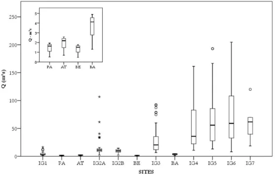
The boxplots for concentration, load, and other variables (T, pH, COND, TURB, Q, SSED, COLIFTOTAL, COLIFFECAL e
SECCHI), in general, showed high variability, a large amount of outliers, and positive asymmetry, suggesting non-normality of the series. Some of these characteristics can be observed in the
low boxplots (data between 2005-2012) presented in Figure 4.
The basin presents a considerable increase of loads and lows downstream the site IG3.
Hypothesis testing
The results of the hypothesis tests are presented in this section. Except in Table 2, in each parameter, the 1st row contains the results for the water quality time series and the 2nd row, the results for the quantity time series. Variables absent from the tables showed no rejection at any monitoring site, and missing points did not show rejection for any variables.
The tests were applied in a total of 720 series (34 variables x 12 sites for quality and 26 variables x 12 sites for loads). The analysis of the results is presented in terms of percentage of rejections and p-values, however, the sites IG7, PA, AT, BE and BA did not present rejections in the tests of seasonality, randomness, and homogeneity, possibly due to the low amount of data (5 observations) and, consequently, lack of evidence for rejection. For these tests the total of series considered for calculation of the percentages of rejection is 420.
Seasonality
Table 2 shows that the seasonal cycle exerts a signiicant
inluence on 9% of the series. In most cases, rejections are observed in both tests. The rejections in NH4+ and N
ORG series
from IG3, T in all sites, and some forms of solids in IG2A are highlighted.
According to the results, the seasonal cycle seems to exert a greater inluence on the organic contribution, represented by variables such as SSV, NH4+, N
ORG and NKEJLDAHL, than in the
hydrological cycle (Q). The smaller inluence on the hydrological cycle is associated with the form of operation to collect information, performed only on business days without the concern of collecting during the occurrence of rainfall. On the other hand, the greater inluence on water quality is associated to signiicant temperature
Figure 4.Boxplots of low rates.
Figure 2. Seasonal distribution of campaigns.
variations and to diffuse pollution, since in the rainy periods, mainly with the irst rains, the contribution of diffuse pollution increases.
Therefore, interferences in the physical, chemical and biological processes throughout the season are expected. This emphasizes the importance of the representativeness of the series, that is, the series should represent all the variability of the parameter or variable being analyzed. The representativity is associated to the frequency of information collections. Thus, irregular collections of low data will hardly represent their temporal variability accurately.
The presence of trend in the series introduces high variability in the groups referring to each station when older data are grouped to the most recent. This makes it dificult to differentiate the groups.
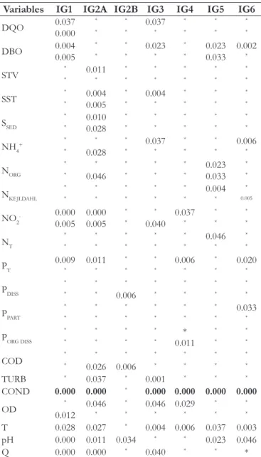
Randomness
It is observed in Table 3 that the randomness hypothesis was rejected in 15% of the series, half with p-value <0.01, especially the COND variable. The low p-values for COND can be explained by the apparent trend of the series, shown in Figure 5.
It is observed that from 2008 the values of conductivity are higher than the median, unlike the older ones. Since the method consists in analyzing the number of oscillations (runs) around the median (4 in this case), the rejections are due to the low number of runs.
This result shows that non-randomness may be a consequence of the analysis of long periods in which the series are non-stationary or non-homogeneous. The increasing trend and non-homogeneity in these series are conirmed by trend and homogeneity tests applied.
The causes for these effects may be real changes in water quality conditions or changes in the form and/or frequency of measurements, methods of analysis, etc., i.e. changes in monitoring
strategy. It emphasizes the importance of investigating the origin of non-randomness.
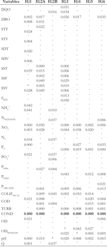
Homogeneity
Table 4 shows the rejection of homogeneity in 26% of the series, half with p-value <0.01. Once again the COND variable is
highlighted. Even if the chance of type I error (rejecting H0 when
this is true) was 10% (α), there would be rejection in several series. The test application method consists of dividing the series in half and comparing the two groups, so the rejections indicate high temporal variability of the series and possible non-stationarity (trend).
The non-homogeneity implies the presence of two or more populations in the same sample, so the p-values, conidence intervals, and other statistical inferences obtained by the analysis of this type of time series do not represent any of the tested populations.
Table 2. Rejection of H0 (equality between seasons) in seasonality tests.
Variables IG1 IG2A IG2B IG3 IG4 IG5 IG6
DQO M2 * * * M2 * *
DBO * * * K2 * K1M1 *
STT * K1M1 * * * * *
STF * K1 * * * * *
SDT * K1M1 * * * * *
SDF * K1 * * * * *
SSF * M2 * * * * *
SSV * * * * K2M2 * K2
NH4+ * K1 * K1M1 K1M1 K1M1 K1M1
NORG K2M2 * * * * K1M1 M2
NKEJLDAHL M2 * * K1 K1M1 K1M1 K1M2
NO2- * K1 * * * * M1
NT * * * * * * M2
TURB K * * M * * *
OD * M1 * * * * *
T KM KM K KM KM KM KM
Q KM * * * * * *
K: Kruskal-Wallis; M: Median test; 1: water quality series; 2: water quantity series. Example: K1M1: rejection of H0 in both tests in water quality series. Some variables do not present numerical distinction, since the load calculation does not apply.
* Non-rejection of H0.
Table 3. Rejections of H0 (series is random) in randomnsess test.
Variables IG1 IG2A IG2B IG3 IG4 IG5 IG6
DQO 0.037
0.000 * *
* *
0.037 *
* *
* *
* *
DBO 0.004
0.005 * *
* *
0.023 *
* *
0.023 0.033
0.002 *
STV ** 0.011* ** ** ** ** **
SST
* *
0.004 0.005
* *
0.004 *
* *
* *
* *
SSED ** 0.0100.028 ** ** ** ** **
NH4+ * *
*
0.028
* *
0.037 *
* *
* *
0.006 *
NORG ** * 0.046
* *
* *
* *
0.023 0.033
* *
NKEJLDAHL ** ** ** ** ** 0.004* 0.005*
NO2- 0.000
0.005 0.000 0.005
* *
* 0.040
0.037 *
* *
* *
NT ** ** ** ** ** 0.046* **
PT 0.009*
0.011 *
* *
* *
0.006 *
* *
0.020 *
PDISS ** ** *
0.006 * *
* *
* *
* *
PPART
* *
* *
* *
* *
* *
* *
0.033 *
PORG DISS ** ** ** ** *
0.011 * *
* *
COD
* *
* 0.026
* 0.006
* *
* *
* *
* *
TURB * 0.037 * 0.001 * * *
COND 0.000 0.000 * 0.000 0.000 0.000 0.000
OD
* 0.012
0.046 *
* *
0.046 *
0.029 *
* *
* * T 0.028 0.027 * 0.004 0.006 0.037 0.003
pH 0.000 0.011 0.034 * * 0.023 0.046
Q 0.000 0.000 * 0.040 * * *
The analysis of historical series should be based on graphical analysis and knowledge about probable causes of non-homogeneity, for example, dates in which there were changes in methods, seasonality, among others.
An alternative to avoid the non-homogeneity of the COND series shown in Figure 5 would be to use part of the series, for example, from the year 2009, unless the objective is trend analysis.
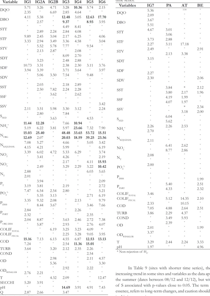
Independence
Rejection of H0 (independence) in favor of H1 (dependence)
was observed in 51% of the series. The test statistics can be seen
in Table 5 and Table 6. Values well above the signiicance level
(1.96) are observed, with emphasis on DBO, NH4+, N
ORG and
COD, which are representative of the organic content of pollution. For the tested series, it is observed that the irregular monitoring frequency in the longer series, predominantly with monthly and quarterly frequencies and long periods of time without data, results in high values of the test statistic with a maximum of 53.72 (Table 5), indicating a strong dependence relationship.
The results of the shorter series indicate that the monthly frequency also provides suficient evidence to reject the hypothesis of independence in several series, however, with considerably lower values of the test statistic, with a maximum value of 17.18 (Table 6).
In water quality, when the sampling frequency is higher (daily, hourly, etc.), there is no evidence that the water quality will be better or worse in the next interval, since the concentrations are not only functions of the lows, but also of the highly variable contributions of loads in the system. On the other hand, when the frequency of monitoring is lower (monthly and quarterly), a certain behavior is expected in terms of water quality due to the seasonality of the climate and the hydrological cycles, which interfere with temperatures, rainfall volume and increased diffuse pollution in the rainier seasons.
These results indicate that the complexity in establishing the dependence ratio may be associated with the increase in the frequency of water quality monitoring. However, due to the seasonal effect, the longer series (greater than one year) may still be correlated. These relationships should be the object of future research.
An alternative for non-rejection of the independence hypothesis in the water quality time series is the analysis of data
separated by season or, according to Gilbert (1987) and McBride
(2005), the use of methods adapted to this characteristic or the use of techniques for the removal of seasonality and trends.
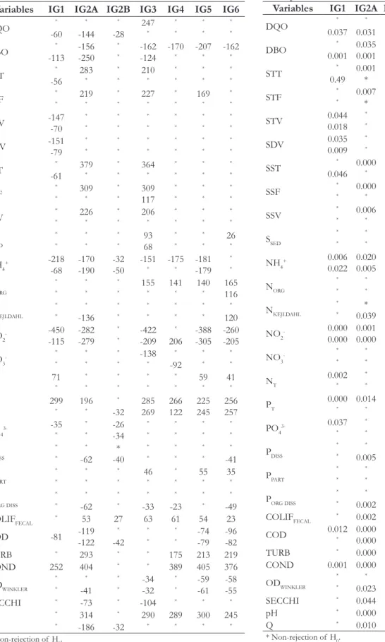
Stationarity
In Table 7 (sites with longer time series), H0 (stationarity)
rejections in favor of H1 (trend) were observed in 31% of the
series (420 series tested). Overall, higher values of the S statistic
are associated with p-values well below 0.05 (Table 8). Of the total
observed rejections, 55% indicate decreasing trend (negative) and 45% increasing trend (positive).
Table 4. Rejections of H0 (homogeneity), in homogeneity test.
Variables IG1 IG2A IG2B IG3 IG4 IG5 IG6
DQO * * * * * 0.016 0.031 0.034 * * * * * *
DBO 0.0020.008 0.017 0.031 * * 0.026 * 0.017 * * * 0.035 * STT * 0.024 0.022 * * * * * * * * * * * STV * 0.004 * * * * * * * * * * * * SDT * 0.020 * * * * * * * * * * * * SDV * 0.006 * * * * * * * * * * * * SST * 0.039 0.000 0.015 * * 0.000 0.006 * * * * * * SSF * * 0.002 0.049 * * 0.006 0.029 * * * * * *
SSV 0.028* 0.005 0.049 * * 0.019 0.006 * * * * * * SSED * * * * * * 0.013 0.050 * * * * * *
NH4+ 0.042
0.041 * * * 0.010 * * * * * * * *
NKEJLDAHL ** * * * 0.037 * * * * * * * 0.006
NO2- 0.000
0.003 0.050 0.028 * * 0.000 0.044 0.000
0.038 0.0020.020 0.006
*
NT *
0.034 * * * 0.037 * * * * * * * *
PT 0.000* ** ** *
0.000 0.027 0.019 * 0.001 0.033 0.000
PO43- 0.021
* * * 0.037 0.006 * * * * * * * *
PDISS ** *
0.027 * 0.004 * * * * * * * * PPART * * * * * * 0.043 * * * 0.012 * 0.008 *
PORG DISS
* * * 0.001 * * * 0.009 * 0.006 * * 0.021 0.013
COLIFFECAL * 0.009 0.045 0.002 0.010 0.014 *
COD 0.021* 0.008
0.001 * 0.004 * * * * 0.020 0.015 0.004 0.001
TURB * 0.000 * 0.000 0.008 0.001 0.001
COND 0.000 0.000 * 0.000 0.000 0.000 0.000
OD 0.021*
* * * * * * * * * * 0.006 *
ODWINKLER ** ** ** *
0.025 0.042 * 0.027 0.005 * 0.005
pH 0.000 0.015 * 0.020 0.008 0.002 0.003
Q 0.001 * 0.037 * * * *
Table 5. Rejections of H0 (independence), sites with longer time series.
Variable IG1 IG2A IG2B IG3 IG4 IG5 IG6
DQO 5.71 2.35 3.26 * 4.71 6.69 3.28 2.85 10.364.64
5.74 *
2.15 *
DBO 4.11*
5.38 2.57 * * 12.48 9.37 3.05 * 12.63 8.93 17.70 3.95
STT ** 2.89* *
2.24 4.49
2.84 8.414.08
* * * * STF 9.89 3.33 2.45 2.94 3.04 3.49 2.17 3.36 6.25 4.58 * * 4.06 3.04 STV * * 5.52 2.13 5.78 2.87 7.77*
*
2.08 9.54* * *
SDT ** *
3.23 * *
8.09 2.48 2.702.88
* * * * SDF 10.73 3.94 3.31 3.39 * * 2.38 3.71 2.30 3.64 3.11 * 3.76 3.97 SDV * * 5.06 * 3.50 * 7.54 * * * 9.48 * * *
SST ** 2.03
2.50 *
7.82 2.182.24
2.89 2.28 * * * * SSF * * * * 3.62 * * * 2.62 * * * * * SSV * 2.11 * 3.51 * 5.98 * 3.30 * 3.12 * * 3.42 2.24
SSED ** 2.80* *
3.63 7.84 * * * * 4.53 * *
NH4+ 11.44 5.19
12.28 6.22
*
3.81 7.665.97 10.94 23.66 * 7.32 * 7.90
NORG 15.03
12.69 25.40 2.07 * * 48.48 20.03 33.65 18.59 53.72 39.25 15.51 23.56
NKEJLDAHL 7.08
4.15 5.27 4.21 * * 4.66 5.99 * * 5.05 * 3.42 6.19
NO2- 3.39 * 6.02 3.41 4.72 * 5.33 4.26 6.29 * * * 3.74 2.19
NO3- * * * 2.49 * * 2.17 3.29 * 2.29 4.11 3.22 15.93 10.42
NT 2.88
2.01 * * * * * * * * 6.03 * 5.65 * PT * 3.19 3.94 3.81 * * * 2.19 * * * * 2.09 2.72
PO43- 7.47
* 6.54 5.35 2.54 3.13 2.80 * * * * 2.71 5.21 6.19
PDISS 3.35* 9.328.44 2.08 3.67 * * 2.13 * * 3.46 9.79 7.66
PPART 2.84
2.32 * * * * * * 2.26 * * 2.35 * *
PORG DISS 2.04*
8.87 5.87 * * 3.63 2.93 2.46 * 2.72 2.76 7.38 4.07
COLIFTOTAL * * 6.19 3.25 3.23 4.09 *
COLIFFECAL * * * 2.25 3.28 9.05 3.95
COD 15.16 7.24 7.13 * 6.13 * 4.55 2.54 6.87 11.36 12.53 15.01 13.13 *
TURB 3.64 * 3.20 2.12 2.35 2.26 *
COND * * * * * 2.54 *
OD * * * * 2.98 5.36 * * * * 2.11 * 4.57 3.30 ODWINKLER * 2.76 * 2.21 * * 2.92 * * * 2.22 * * *
T * * 4.32 2.09 * * 12.47
SECCHI 5.20 3.91 * * * * *
pH * * * 14.69 3.91 4.91 7.43
Q 2.87 2.66 * 3.47 * * *
* Non-rejection of H0.
Table 6. Rejections of H0 (independence), sites with shorter time series.
Variables IG7 PA AT BE BA
DQO 5.36 2.09 * * 3.54 * * * 5.21 * DBO 3.67 5.51 * * * * * * * *
STT 4.67* 3.01
3.06 * * * * * * STF 3.73 2.27 2.88 3.11 * 17.18 * * * *
STV 2.49*
* 2.13
*
3.38 2.91*
2.41 *
SDT 3.15* ** ** ** **
SDF * 2.27 * * * * * * * *
SDV 2.30*
* * * * 2.06 * * *
SST ** 3.843.80 *
2.17 2.12 1.96 5.12 * SSF * * 4.19 4.07 1.99 1.97 * * 3.87 * SSV * * * * *
3.18 2.342.00
8.85
*
SSED ** 6.04
5.62 * * * * * *
NH4+ 2.26 2.70 2.26 * 2.53 * * * 2.80 *
NKEJLDAHL *
2.11 * * * * * * * *
NO2- *
*
6.41
8.77 2.622.86
* *
2.79 *
NT 2.08* ** ** ** **
PO43- 2.00
* * * * * * * * *
PDISS ** ** ** *
1.99 * * PPART * * 5.40 4.33 * * 2.51 2.32 4.22 *
COLIFTOTAL 3.46 * * * 14.44
COLIFFECAL * 5.12 14.35 2.10 *
COD 2.33
7.05
*
4.88 10.152.64 * 2.51
5.23 *
TURB 3.86 2.29 4.37 * *
COND * 3.49 5.93 * *
OD * 2.01 2.39 * * * * 1.99 * *
ODWINKLER 3.37*
* * * * * * * 3.31
T 3.29 2.44 2.24 3.33 2.67
pH 1.97 * * 4.96 2.69
* Non-rejection of H0.
Table 7. Rejections of H0 (stationarity), sites with longer time series, S statistic.
Variables IG1 IG2A IG2B IG3 IG4 IG5 IG6
DQO * -60 * -144 *
-28 247* * * * * * * DBO * -113 -156 -250 * * -162 -124 -170 * -207 * -162 * STT * -56 283 * * * 210 * * * * * * * STF * * 219 * * * 227 * * * 169 * * * STV -147 -70 * * * * * * * * * * * * SDV -151 -79 * * * * * * * * * * * * SST * -61 379 * * * 364 * * * * * * * SSF * * 309 * * * 309 117 * * * * * *
SSV ** 226* ** 206* ** ** **
SSED * * * * * * 93 68 * * * * 26 *
NH4+ -218
-68 -170-190 -32 -50 -151 * -175 * -181 -179 * *
NORG ** * * * * 155 * 141 * 140 * 165 116
NKEJLDAHL ** *
-136 * * * * * * * * * 120
NO2- -450 -115 -282 -279 * * -422 -209 * 206 -388 -305 -260 -205
NO3- * * * * * * -138 * * -92 * * * *
NT 71* ** ** ** ** 59* 41*
PT 299* 196* *
-32 285 269 266 122 225 245 256 257
PO43- -35
* * * -26 -34 * * * * * * * * PDISS * * * -62 * -40 * * * * * * * -41 PPART * * * * * * 46 * * * 55 * 35 *
PORG DISS
* * * -62 * * * -33 * -23 * * * -49
COLIFFECAL * 53 27 63 61 54 23
COD -81 -119
-122 * -42 * * * * -74 -79 -96 -82
TURB * 293 * * 175 213 219
COND 252 404 * * 389 405 376
ODWINKLER * * * -41 * * -34 -32 * * -59 -61 -58 -55
SECCHI * -73 * -104 * * *
pH * 314 * 290 289 300 245
Q * -186 -32 * * * *
* Non-rejection of H0.
Table 8. Rejections of H0 (stationarity), sites with longer time series, p-values.
Variables IG1 IG2A IG2B IG3 IG4 IG5 IG6
DQO * 0.037 * 0.031 * 0.032 0.002 * * * * * * * DBO * 0.001 0.035 0.001 * * 0.026
0.028 0.020 0.006 0.011
STT * 0.49 0.001 * * * 0.009 * * * * * * * STF * * 0.007 * * * 0.006 * * * 0.025 * * *
STV 0.0440.018 ** ** ** ** ** **
SDV 0.035 0.009 * * * * * * * * * * * * SST * 0.046 0.000 * * * 0.000 * * * * * * * SSF * * 0.000 * * * 0.000 0.050 * * * * * *
SSV ** 0.006* ** 0.011* ** ** **
SSED * * * * * * 0.025 0.049 * * * * 0.040 *
NH4+ 0.006
0.022 0.020 0.005 0.016 0.000 0.040 * 0.018 * 0.015 0.013 * *
NORG ** ** ** 0.036* 0.039* 0.046* 0.010
0.037
NKEJLDAHL ** * 0.039 * * * * * * * * * 0.033
NO2- 0.000
0.000 0.001 0.000 * * 0.000 0.002 * 0.000 0.000 0.000 0.000 0.002
NO3- * * * * * * 0.037 * * 0.036 * * * *
NT 0.002* ** ** ** ** 0.008* 0.036*
PT 0.000*
0.014 * * 0.016 0.001 0.000 0.001 0.025 0.005 0.001 0.000 0.000
PO43- 0.037
* * * 0.043 0.012 * * * * * * * * PDISS * * * 0.005 * 0.004 * * * * * * * 0.024
PPART ** ** ** 0.032* ** 0.013* 0.046*
PORG DISS
* * * 0.002 * * * 0.040 * 0.043 * * * 0.003 COLIFFECAL * 0.002 0.020 0.000 0.001 0.002 0.011
COD 0.012*
0.000 0.000 * 0.002 * * * * 0.020 0.014 0.002 0.004
TURB * 0.000 * * 0.017 0.005 0.001
COND 0.001 0.000 * * 0.000 0.000 0.000
ODWINKLER * * * 0.023 * * 0.034 0.016 * * 0.002 0.001 0.001 0.001
SECCHI * 0.044 * 0.045 * * *
pH * 0.000 * 0.001 0.000 0.000 0.001
Q * 0.010 0.016 * * * *
* Non-rejection of H0.
From IG1 to IG6, increasing trends are concentrated on variables such as NORG, NT, PT, COLIFFECAL, COND, TURB and pH, indicating the increasing contribution of organic matter in the basin. Decreasing trends are observed in variables such as DBO,
NH4
+, NO 2
-, PO 4
3-, P
DISS, PORG DISS and COD, which represent the
products of decomposition.
not relect seasonal effects. It is important to note that these series were obtained by the same monitoring strategy and under the same seasonal conditions as the other series, evidencing the existence of other factors that determine their attendance. The absence of seasonality is associated with the non-representativeness, mainly, of the low series. The low series in the Iguaçu River basin show seasonal variations.
The understanding of the applied methods allowed the establishment of relations of cause and effect between randomness, homogeneity and independence and presence or not of seasonality and trends. Seasonality may give rise to cyclical (non-random) variability, to data signiicantly higher or lower in different (heterogeneous) seasons, and to data decreasing or increasing in a chronological sequence as they approach a particular season of the year (dependence).
The presence of trends may produce signiicant differences between recent and old data (non-homogeneity), its slope may result in few runs (not randomness), and make predictable part of the variability of future data depending on the last data obtained (dependence).
However, the results show that seasonality and trend can not assess the assumptions of randomness, homogeneity, and independence alone. Table 10 shows that the absence of seasonality and trends in the low series are associated with compliance with all assumptions in IG4, IG5 and IG6, but not in IG3. The lack of trend may be associated to non-attendance, as in IG1, but also to compliance, as in IG4, IG5 and IG6. In this way, it is understood that all assumptions must be tested prior to frequency analysis in water quality time series. Some causes of non-compliance with basic assumptions can be veriied graphically as well as possible solutions to work around the problem.
CONCLUSIONS
The veriication of the basic assumptions for frequency analysis in water quality series in the Upper Iguaçu Basin evidenced the need for a more cautious approach to the analysis of large databases. The assumption of randomness, homogeneity, independence and stationarity premises, typical in studies of water quality, can be misleading in most of the series.
The applications of the tests allowed the identiication of series important characteristics, as well as, reveled deiciencies of the typical strategies of water quality monitoring. The fulillment of the basic assumptions for the analysis of water quality time series is essentially related to the monitoring strategies and techniques of approach of the series for analysis. As surface water quality variability is strongly related to anthropogenic activities, monitoring strategies should generate information on the cycles of variation corresponding to the various activities of man, i.e. daily and weekly cycles, as well as holidays.
Likewise, the annual cycle, due to seasonality, and other events that signiicantly interfere with water quality conditions through diffuse pollution should also be monitored. The data for each cycle or event should be compared and, if they are signiicantly different, separately analyzed.
However, due to the high costs, the intrinsic dificulties of monitoring and the lack of planning, the typical monitoring
Table 9. Rejections of H0 (stationarity), sites with shorter time series, S statistic (p-value).
Variable IG7 PA AT BE BA
STT ** 8 (0.043)* ** 8 (0.042)8 (0.042) *
8
(0.042)
STF ** 8 (0.043)* ** 8 (0.042)* **
STV **
8 (0.042)
10 (0.014)
* *
* *
* *
SDT ** 8 (0.042)8 (0.042) **
* 10
(0.008)
*
8
(0.042)
SDF ** **
* 10
(0.008)
*
8 (0.042)
*
8
(0.042)
SDV
* *
8 (0.042) 8 (0.042)
* *
* *
* *
NORG ** ** 8 (0.042)* **
*
8
(0.042)
NO2- *
*
*
8 (0.043)
* *
* *
* *
NT **
* *
* *
*
8 (0.042)
*
8
(0.042)
PT
* *
* 10
(0.008)
* *
*
8 (0.042)
* *
PPART
* *
* *
* *
* *
-8
(0.043) *
COD
* *
-6 (0.045)
*
* *
* 10 (0.014)
*
8
(0.042)
TURB * * * * -8
(0.042)
COND * 8 (0.043) 6 * *
T 10 (0.014) 10
(0.014) 8 (0.043) *
8
(0.043)
* Non-rejection of H0.
biodegradability, consistent with the increasing trend observed in the pH variable, which negatively affects the action of microorganisms.
Synthesis of results
Almost all water quality variables were rejected in at least one of the assumptions at most monitoring sites. Some series, such as the STT and Q at IG6, met all the assumptions and did
Table 10. Comparison among rejections in tests for low Q.
Test IG1 IG2A IG2B IG3 IG4 IG5 IG6
R 0.000 0.000 * 0.040 * * *
H 0.001 * 0.037 * * * *
I 2.87 2.66 * 3.47 * * *
T * -186 -32 * * * *
S KM * * * * * *
R: randomness, H: homogeneity, I: independence, T: trend, S: seasonality, KM: rejection of hypothesis of equality among seasons by Kruskal-Wallis and median
strategies involve irregular frequencies, monitoring only on working days (representing around 24% of the time of one year), absence of collection in periods of heavy rain, night periods, holidays, weekends and summer, which together represent most of the time in a year.
The time series generated from these strategies represent only part of the daily cycle (commercial hours) and their seasonality, not being able to provide information on other periods. Direct analysis of these series often produces non-representative statistics, as they do not meet the basic assumptions of randomness, homogeneity, independence and stationarity.
Among the possible solutions are the separation of the data into groups, the application of trend and seasonality removal techniques and the transformation into annual series by means of averages or medians. However, irregular frequencies, without planning, negatively interfere in this process. In general, there is little data in the summer and data are concentrated irregularly between stations. This makes it dificult to characterize the seasonality and makes the mean and median biased.
The results point to the need to rethink the way water quality monitoring networks operate, especially regarding the frequency of sample collection, in order to have representative data.
The knowledge on this topic in the area of water quality is still incipient, with many questions still unanswered, such as: which tests are most appropriate for checking the assumptions? how do the sampling frequencies interfere in the tests of randomness, homogeneity, independence and stationarity? what other factors besides seasonality and trends lead to non-randomness, non-homogeneity, dependence and non-stationarity? what is the best strategy for monitoring and analyzing data when resources are scarce?
ACKNOWLEDGEMENTS
The authors thank the Coordination of Improvement of Higher Education Personnel (CAPES), the National Council for Scientiic and Technological Development (CNPq), and the editors and reviewers responsible for a constructive review process, committed to the quality of information, generating signiicant contributions for these research.
REFERENCES
AMERICAN PUBLIC HEALTH ASSOCIATION – APHA. American Water Works Association – AWWA. Water Environment Federation – WPCF, Standard methods for the examination of water and wastewater. Washington, 1999.
CHADEE, J. C.; SHARMA, C. Fitting flexible wind speed models:
a new approach. In: WELLS, J. (Ed.). Solutions for energy security &
facility management challenges. Lilburn: The Fairmont Press, 2003. p. 249.
COELHO, M. Estratégia de monitoramento da qualidade da água para
a gestão de recursos hídricos em bacias urbanas. 2013163 f. Dissertation (Environmental and Water Resources Engineer) - Federal University of Paraná, Curitiba, 2013.
COSTA, M. P.; OLIVEIRA, R. B. S.; SOUZA, M. L. Análise da Tendência do Índice de Qualidade das Águas da Região Hidrográfica
do Paraná no Período 2000-2009. In: BRAZILIAN SYMPOSIUM
ON WATER RESOURCES, 29., 2011, Maceió. Proceedings... São
Paulo: ABRH, 2011. Available from: <http://www.abrh.org.br/ SGCv3/index.php?PUB=3&ID=81&PAG=1>. Access on: 26 may 2015.
DAHM, K. G.; GUERRA, K. L.; MUNAKATA-MARR, J.;
DREWES, J. E. E. Trends in water quality variability for coalbed
methane produced water. Journal of Cleaner Production, v. 84, p.
840-848, 2014. http://dx.doi.org/10.1016/j.jclepro.2014.04.033.
FORMIGONI, Y., BRITES, A. P. Z.; FERNANDES, C. V. S.;
PORTO, M. F. A. Análise crítica da curva de permanência de qualidade da água com base em dados históricos. In: BRAZILIAN SYMPOSIUM ON WATER RESOURCES, 29., 2011, Maceió.
Proceedings... São Paulo: ABRH, 2011. Available from: <http:// www.abrh.org.br/SGCv3/UserFiles/Sumarios/ec99f1061725d6 3695b7bea3067296d4_31aef3f050dfe0930e76fff29fa8b397.pdf>. Access on: 26 may 2015.
GILBERT, R. O. Statistical methods for environmental pollution monitoring. John Wiley & Sons, 1987.
GONÇALVES, V. D., FERNANDES, C. V. S.; KNAPIK, H.
G.; MÄNNICH, M. Desafios da gestão de recursos hídricos: um
olhar sobre o monitoramento ambiental de rios. In: BRAZILIAN CONGRESS OF SANITARY AND ENVIRONMENTAL
ENGINEERING, 26., 2011, Porto Alegre. Proceedings... São
Paulo: ABES, 2011.
HAMED, K. H.; RAO, A. R. A modified Mann-Kendall trend test
for autocorrelated data. Journal of Hydrology, v. 204, n. 1-4, p.
182-196, 1998. http://dx.doi.org/10.1016/S0022-1694(97)00125-X.
HELSEL, D. R.; HIRSCH, R. M. Statistical methods in water resources:
techniques of water resources investigations of the United States Geological Survey. Reston: US Geological Survey, 2002. chap.A3.
Book 4: Hydrologic analysis and interpretation. Available from: <http://pubs.usgs.gov/twri/twri4/>. Access on: 2 apr. 2013.
HIRSCH, R. M.; MOYER, D. L.; ARCHFIELD, S. A. Weighted Regressions on Time, Discharge, and Season (WRTDS), with an
Application to Chesapeake Bay River Inputs1. JAWRA Journal
of the American Water Resources Association, v. 46, n. 5, p. 857-880,
2010. PMid:22457569. http://dx.doi.org/10.1111/j.1752-1688.2010.00482.x.
HULLEY, M.; CLARKE, C.; WATT, E. Low flow frequency
analysis for streams with mixed populations. Canadian Journal
of Civil Engineering, v. 42, n. 8, p. 503-509, 2015. http://dx.doi. org/10.1139/cjce-2014-0323.
KNAPIK, H. G.; FERNANDES, C. V. S.; AZEVEDO, J. C. R.
<http://www.abrh.org.br/SGCv3/index.php?PUB=3&ID=1 55&PUBLICACAO=SIMPOSIOS>. Access on: 26 may 2015.
KONDAGESKI, J. H.; FERNANDES, C. V. S. Calibração de
Modelo de Qualidade da Água para rio utilizando Algoritmo Genético: Estudo de caso de Rio Palmital-PR. Brazilian Journal of Water Resources, v. 14, n. 1, p. 63-73, 2009.
MARIN, M. C. F C.; SCUISSIATO, C.; FERNANDES, C. V.
S.; PORTO, M. F. A. Proposta preliminar de reenquadramento dos corpos de água em classes e avaliação do seu risco de não atendimento: estudo de caso da Bacia do Alto Iguaçu. In: BRAZILIAN SYMPOSIUM ON WATER RESOURCES, 17.,
2007, São Paulo. Proceedings... São Paulo: ABRH, 2007. Available
from: http://www.abrh.org.br/SGCv3/index.php?PUB=3&ID= 155&PUBLICACAO=SIMPOSIOS>. Access on: may 26, 2015.
MCBRIDE, G. B. Using statistical methods for water quality management.
New Jersey: John Wiley & Sons, 2005.
MERZ, B.; THIEKEN, A. H. Separating natural and epistemic
uncertainty in flood frequency analysis. Journal of Hydrology,
v. 309, n. 1-4, p. 114-132, 2005. http://dx.doi.org/10.1016/j. jhydrol.2004.11.015.
NAGHETTINI, M.; PINTO, E. J. A. Hidrologia e estatística. geological survey of Brazil. Belo Horizonte: CPRM, 2007.
PITRAT, D. M. J. J. Avaliação da contaminação por metais em rios: estudo
de caso da Bacia do Rio Passaúna. 2010. 231 f. Dissertation (Water Resources and Environmental Engineering) - Federal University of Paraná, Curitiba, 2010.
SIEGEL, S.; CASTELLAN JUNIOR, N. J. Estatística não paramétrica para ciências do comportamento. 2nd ed. Porto Alegre: Artmed, 2006.
TORRES, I. C.; LEMOS, R. S.; MAGALHÃES JUNIOR, A. P.
Influence of the Rio Taquaraçu in the water quality of the Rio das Velhas: subsidies for reflections of the case of water shortage in Belo Horizonte metropolitan region–MG, Brazil. Brazilian Journal of Water Resources, v. 21, n. 2, p. 429-438, 2016.
VIEIRA, J.; FONSECA, A.; VILAR, V. J. P.; BOAVENTURA, R.
A. R.; BOTELHO, C. M. S. Water quality modelling of Lis River,
Portugal. Environmental Science and Pollution Research International,
v. 20, n. 1, p. 508-524, 2013. PMid:23001788. http://dx.doi. org/10.1007/s11356-012-1124-5.
WANG, Y.; WANG, P.; BAI, Y.; TIAN, Z.; LI, J.; SHAO, X.;
MUSTAVICH, L. F.; LI, B.-L. Assessment of surface water quality via multivariate statistical techniques: a case study of the
Songhua River Harbin region, China. Journal of Hydro-environment
Research, v. 7, n. 1, p. 30-40, 2013. http://dx.doi.org/10.1016/j. jher.2012.10.003.
Authors contributions
Marcelo Coelho: Literature review, writing, running the statistical tests, analysis of results, method development, conclusions and translation.
Cristovão Vicente Scapulatempo Fernandes: Advisor, analysis of results and conclusions and translation.
Daniel Henrique Marco Detzel: Advisor, analysis of results and conclusions and translation.