On the Existence of Pure Strategy Nash
Equilibria in Large Games
∗
Guilherme Carmona
Universidade Nova de Lisboa
December 21, 2004
Abstract
We consider an asymptotic version of Mas-Colell’s theorem on the existence of pure strategy Nash equilibria in large games. Our result states that, if players’ payoff functions are selected from an equicon-tinuous family, then all sufficiently large games have an ε – pure, ε – equilibrium for all ε > 0. We also show that our result is equivalent to Mas-Colell’s existence theorem, implying that it can properly be considered as its asymptotic version.
1
Introduction
Nash (1950)’s celebrated existence theorem asserts that every finite normal form game has a mixed strategy equilibrium. However, in many contexts mixed strategies are unappealing and hard to interpret, leading naturally to the question of the existence of pure strategy Nash equilibria.
Regarding games with a finite action space, considered by Nash (1950), Schmeidler (1973) was successful in obtaining an answer to the above ques-tion. He showed that in a special class of games — in which each player’s payoff depends only his choice and on the average choice of the others — a pure strategy Nash equilibrium exists in every such game with a continuum of players.
∗I wish to thank Myrna Wooders for very helpful comments and John Huffstot for
Later, Mas-Colell (1984) extended Schmeidler’s Theorem to a broader class of games by allowing players’ payoff to depend on the distribution of choices made by the others.1 At almost the same time, Rashid (1983)
ob-tained an asymptotic version of Schmeidler’s theorem, according to which all sufficiently large games of the same class considered by Schmeidler (1973) have an approximately pure, approximate equilibrium provided that players’ payoff functions are selected from an equicontinuous family.2
Asymptotic results are important because, after all, real-world games have finitely many players. Therefore, we ask whether or not there is an asymptotic version for Mas-Colell’s Theorem that parallels Rashid’s version of Schmeidler’s Theorem.
Our Theorem 1 answers the above question affirmatively. It states that if players’ payoff functions are selected from an equicontinuous family, then all sufficiently large games of the same class considered by Mas-Colell (1984) have an ε – pure, ε – equilibrium for all ε > 0.
This result thus provides an approximate version of Mas-Colell’s theo-rem. Despite the similarities, there are nevertheless some differences: our assumption on the number of players is less extreme, but our conclusion is weaker and requires an equicontinuity assumption. So, is our result really a version of Mas-Colell’s?
Again, the answer is yes: our Theorem 3 shows that the two results are equivalent, i.e., that each one follows from the other. This means that they are simply two different ways of expressing the same phenomenon: the existence of pure strategy Nash equilibria can be addressed either in its exact version in games with a continuum of players or in an approximate version in large, equicontinuous games.
This remark reinforces the main conclusion we obtained in Carmona (2004a). There we showed that in the same class of games we consider here, Nash equilibria of games with a continuum of players are the limit points of approximate equilibria of similar large finite games. Given this, the
1More precisely, Mas-Colell’s Theorem asserts that an equilibrium distribution exists whenever the action space is a compact metric space. In the special case considered by Schmeidler (1973), an equilibrium strategy can be obtained from the equilibrium distri-bution.
2More precisely, Rashid’s Theorem shows that all Nash equilibria of sufficiently large games of the same class can be approximately purified. Note that, as we have shown in Carmona (2004b), Rashid’s Theorem requires that players’ payoff functions be selected from an equicontinuous family.
equivalence asserted by our Theorem 3 becomes quite natural.
It is useful to compare our asymptotic result to others obtained in the literature. The equivalence between it and Mas-Colell’s implies that it is more general than Schmeidler’s Theorem. It is also more general than Rashid’s result on the existence of approximately pure, approximate equilibria in large, equicontinuous games. In both cases, this follows simply because we consider a more general framework.
The existence of approximately pure, approximate equilibria in large, equicontinuous games follows also from the work of Kalai (2001) and Cartwright and Wooders (2003). Although the class of games considered by them differs from ours, we can nevertheless approximate equicontinuous games in their class by equicontinuous games in ours (this approximation requires that we focus on a sub-class in which all players have the same finite action space and there is no move by nature, assumptions that are not made by those au-thors). This implies that the existence of approximately pure, approximate equilibria in large, equicontinuous games in their framework satisfying the above assumptions follows also from our Theorem 1.
We consider several possible extensions for our work. Motivated by the above relationship with the papers of Rashid (1983), Kalai (2001) and Cartwright and Wooders (2003) we ask whether or not we can approximately purify all Nash equilibria of large, equicontinuous games, as they can. Our Theorem 4 shows that, in general, we cannot. This implies that our Theorem 1 is not more general than their main results, but only to the corollaries on the existence of approximately pure, approximate equilibria in large, equicon-tinuous games that can be obtained from them.3
Finally, we provide examples that show that neither can we obtain an exact version for our Theorem 1 (i.e., with ε = 0), nor can we dispense with the equicontinuity assumption.
2
Notation and Definitions
In the class of normal-form games we consider, all players have the same strategy space: the standard unit simplex ∆m on Rm, m > 1. As usual,
3It is worth emphasizing that both Kalai (2001) and Cartwright and Wooders (2003) allow moves by nature and different players to have different action spaces. Furthermore, Cartwright and Wooders (2003) allow players to have denumerable action spaces. These are aspects in which their analysis is more general than ours.
the interpretation is that there are m pure strategies which are identified with the vertices E = {e1, . . . , em} of ∆m, and players can randomize over it.
Since the focus is on a property that depends on the number of players, we will index any game by the number of its players. Thus, Gnis a normal-form
game in which the set of players is Tn = {1, . . . , n}, and each has ∆m as its
choice set. A strategy is then a function x : {1, . . . , n} → ∆m. Obviously, a
strategy x can also be thought of as the vector (x1, . . . , xn) in ∆nm.
A game Gnis then specified by the vector of payoff functions, one for each
player. We denote player t’s payoff function by Ut, for any t ∈ Tn; therefore,
Gn is described by the vector (Ut)t∈Tn. If we let Gn denote the set of all functions g : ∆n
m → R and G = ∪∞n=1Gn, then a game Gn can be thought of
as a subset of Gn, and so of G.
In this paper we will focus on a special class of games in which each player’s payoff depends on his strategy and on the distribution of strategies chosen by the other players. Let M be the set of Borel probability measures on ∆m endowed with the Prohorov metric ρ.4 Given a strategy x in a game
with n players and t ∈ Tn, we define νn,t◦ x−1 ∈ M as follows:
νn,t◦ x−1(B) =
|{j ∈ Tn\ {t} : xj ∈ B}|
n − 1 (1)
for any Borel set B ⊆ ∆m. To each player t, we associate m continuous
functions Vtk : M → R, 1 ≤ k ≤ m; then player t’s payoff function is
Ut(x) = xt1Vt1(νn,t◦ x−1) + . . . + xtmVtm(νn,t◦ x−1), (2)
for any strategy x. We denote this class of games by H.
Note that a game Gn ∈ H is described by the vector (Vtk)t,k. We let
V (Gn) = {Vtk : 1 ≤ t ≤ n, 1 ≤ k ≤ m} and so V (Gn) is a subset of U, the
space of all continuous, real-valued functions on M.
The class of games considered by Rashid (1983) is easily seen to be a special case of our framework. Let ¯f : M → ∆m be defined by ¯f (µ) =
R
∆midµ, where i : ∆m → ∆m denoted the identity function. Assume that Gn is such that for every k ∈ {1, . . . , m} and t ∈ Tn, there exists a function
Rtk : R → R such that Vtk(µ) = Rtk µ n − 1 n f (µ)¯ ¶ , (3)
for all µ ∈ M. In such a game, then ¯ f (νn,t◦ x−1) = X j6=t xj n − 1, (4) and so Ut(x) = xt1Rt1 à X j6=t xj n ! + . . . + xtmRtm à X j6=t xj n ! , (5)
for any strategy x. We will denote this class of games by R. For any ε ≥ 0, we say that x∗ = (x∗
1, . . . , x∗n) is an ε – equilibrium of a
game Gn if, for all t ∈ {1, . . . , n},
Ut(x∗) ≥ Ut(xt, x∗−t) − ε for all xt ∈ ∆m. (6)
Thus, in an ε – equilibrium all players are close to their optimum by choosing according to x∗. A strategy x∗ is a Nash equilibrium of G
n if x∗ is an ε –
equilibrium of Gn for ε = 0.
For any strategy x in a game Gn, let Pn(x) = {t ∈ Tn: xt∈ E}. We say
that x is ε – pure if
|Pc n(x)|
n < ε. (7)
That is, in an ε – pure strategy all but a small fraction of players play a pure strategy.
Let x∗ be a Nash equilibrium of a game G
n. Then, we say that x is an ε
– purification of x∗ if x is an ε – pure, ε – equilibrium and
||U(x) − U(x∗)|| < ε. (8)
Let K be a subset of U. We say that K is equicontinuous (or, that the family K of functions is equicontinuous) if for all η > 0 there exists a δ > 0 such that
||V (x) − V (y)|| < η
whenever ρ(x, y) < δ, x, y ∈ M and V ∈ K (see Rudin (1976, p. 156)). In our framework, equicontinuity can be interpreted as placing “a bound on the diversity of payoffs” (see Khan, Rath, and Sun (1997)).
3
Existence of Approximately Pure,
Approx-imate Equilibria in Large, Equicontinuous
Games
In this section we state our first main result. It says that all sufficiently large games have an ε – pure, ε – equilibrium, provided that players’ payoff functions are selected from an equicontinuous family.
Theorem 1 Let K be an equicontinuous subset of U. Then, for all ε > 0 and all m ∈ N there exists N ∈ N such that n ≥ N and V (Gn) ⊆ K implies
that Gn has an ε – pure, ε – equilibrium.
Theorem 1 is an approximation result: it guarantees the existence of an approximate equilibrium that is approximately pure if the game is sufficiently large. Essentially, we are approximating not only pure strategy Nash equi-libria, but also games with a continuum of players, in which the conclusion of Theorem 1 holds exactly. This is how we proceed: we associate, to any sufficiently large finite game, a game with a continuum of players having the same distribution of payoff functions. In such a game, we restrict players to play pure strategies and, by Mas-Colell (1984)’s existence theorem, we ob-tain an equilibrium distribution. We then use this equilibrium distribution to construct an approximately pure, approximate equilibrium for the original finite game.5
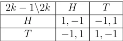
Our construction shows that we can think of Theorem 1 as being an asymptotic version of Mas-Colell (1984)’s existence theorem. As we have emphasized in Carmona (2004a), such asymptotic results are natural since we can characterize the Nash equilibria of games with a continuum of players in terms of approximate equilibria of games with a finite number of players. Another aspect that stresses the asymptotic nature of Theorem 1 is that it requires a class of payoff functions for which an equilibrium is sure to exist whenever the game has a continuum of players. In particular, it is false for games in which players have general payoff functions. As a simple example, consider ε = 1/4, and the following games Gn with m = 2 and n even:
players’ 2k and 2k − 1, 1 ≤ k ≤ n/2, play the matching pennies, i.e., their payoff depend only on their choices and is given by:
2k − 1\2k H T
H 1, −1 −1, 1
T −1, 1 1, −1
Table 1: Payoff Function for the Matching Pennies
Then, if x is a 1/4 – pure strategy, it follows that there is 1 ≤ k ≤ n/2 such that both players 2k − 1 and 2k play a pure strategy. This implies that x cannot be an 1/4 – equilibrium. Therefore, Gn has no 1/4 – pure, 1/4 –
equilibrium for all n even.
In general, Theorem 1 is also false if we insist on ε = 0, or if we drop the equicontinuity assumption. This will be established by the example in Section 6.
It is also useful to compare Theorem 1 to other results in the literature. It follows from Rashid (1983)’s Theorem that the conclusion of Theorem 1 holds for games in R. Since we do not require that payoffs depend only on the average choice of the other players, Theorem 1 is more general in this respect.6
Theorem 1 also provides similar generalizations for other classes of games that have been considered. Before we can state them, we need a slight generalization of the theorem.
Let C ⊆ G and K ⊆ U. Then C can be approximated by (H, K) if the following property holds: For all ε > 0 there exists N ∈ N such that if n ≥ N and Fn= (Utk)t,k∈ C there exists Gn ∈ H satisfying V (Gn) ⊆ K and
||V (x) − U(x)|| < ε (9)
for all strategies x : {1, . . . , n} → ∆m. The following corollary is an obvious,
but useful, consequence of the above definition.
Corollary 1 Let K be an equicontinuous subset of U and assume that C ⊆ G can be approximated by (H, K). Then, Theorem 1 holds for C.
That is, for all ε > 0 and all m ∈ N there exists N ∈ N such that n ≥ N and Gn ∈ C implies that Gn has an ε – pure, ε – equilibrium.
6Note that although not explicitly stated, Rashid’s Theorem requires that players’ payoff functions are selected from an equicontinuous family. For details, see Carmona (2004b).
Corollary 1 is useful for extending Theorem 1 to other classes of games. A class in which we are interested consists of a particular case of the one considered in Kalai (2001) and Cartwright and Wooders (2003) (see footnote 3). We will let K be the class of the following games: A game Gn ∈ K
is defined by the vector (ftk)t,k where ftk : ∆m → R is continuous for all
1 ≤ t ≤ n and 1 ≤ k ≤ m. For c = (c1, . . . , cn) ∈ En, e ∈ E and t ∈ Tn,
define
empc−t(e) = |{i 6= t : ci = e}|
n − 1 . (10)
Then, for any strategy x, define
Ut(x) = xt1Ut1(x−t) + . . . + xtmUtm(x−t), (11) and Utk(x−t) = X c−t∈Qi6=tEi à Y i6=t xi(ci) ! ftk(empc−t). (12)
Let V be the space of all continuous functions f : ∆m→ R and F (Gn) =
{ftk : 1 ≤ t ≤ n, 1 ≤ k ≤ m} ⊆ V for any Gn∈ K.
Let D be an equicontinuous subset of V. Define K ⊆ U as follows K = {f ◦ ¯f : f ∈ D}. Then, K is an equicontinuous subset of U. Let C be the subset of K induced by D, i.e., all the games Gn= (ftk)t,k satisfying ftk ∈ D
for all 1 ≤ t ≤ n and 1 ≤ k ≤ m. It then follows from Kalai (2001, Lemma 4) that C can be approximated by (H, K). Hence, the conclusion of Theorem 1 holds for the class K, provided that the payoff functions are derived from an equicontinuous family of functions.
We conclude this section with another class of games. This class of games is very similar to the one we consider in Theorem 1, since games in the two classes differ only on the definition of the distribution of actions that affects players’ payoffs.
Let Gnbe a game and x a strategy. We let νndenote the uniform measure
on Tn, and so we define νn◦ x−1 ∈ M as follows:
νn◦ x−1(B) = |{t ∈ Tn: xt∈ B}|
n (13)
for any Borel set B ⊆ ∆m. To Gn we associate the game Gn defined as
follows: it has the same set of players Tn and each has the same action space
∆m. For t ∈ Tn, his payoff function is now
for any strategy x. Thus, in Gn player t’s payoff depends on the distribution
of actions played by all players, including t himself, whereas in Gnit depends
only on the distribution induced by the choices of the other players. Note, however, that V (Gn) = V (Gn). We let H denote this class of games.
The following remark states that the conclusion of Theorem 1 also holds for H. In fact, Lemma 3 in Appendix A.2 shows that it is equivalent to Theorem 1.
Remark 1 Let K be an equicontinuous subset of U. Then, for all ε > 0 and all m ∈ N there exists N ∈ N such that n ≥ N and V (Gn) ⊆ K implies that
Gn has an ε – pure, ε – equilibrium.
Note that in a game Gn ∈ H, each player’s payoff function is linear in
his own choice. Since this is not necessarily the case in Gn, Remark 1 shows
that the the existence of approximately pure, approximate equilibria in large games does not depend on that assumption.
4
On the Equivalence to Mas-Colell’s
Theo-rem
We have emphasized that Theorem 1 can be thought of as an asymptotic version of Mas-Colell (1984)’s existence theorem. Moreover, we have used it in our proof, and so it follows that Theorem 1 is implied by it. In this section we show that the two results are equivalent.
We next describe Mas-Colell (1984)’s Theorem in our context, i.e., in games with a finite number of pure strategies. We note that his theorem holds more generally, and therefore, our Theorem 1 is really equivalent to a particular version of it.
Let E be the space of the continuous functions u : E × M(E) → R. A game with a continuum of players is described by a Borel probability measure on E.
Given a Borel probability measure τ on E × E, we denote by τE and τE
the marginal distributions of τ on E and E respectively. The expression u(e, τ ) ≥ u(E, τ ) means u(e, τ ) ≥ u(e0, τ ) for all e0 ∈ E.
Given a game µ, a Borel probability measure τ on E × E is an equilibrium distribution for µ if
2. τ ({(u, e) ∈ E × E : u(e, τE) ≥ u(E, τE)}) = 1.
Mas-Colell (1984)’s Theorem 1 asserts the existence of an equilibrium distribution in games with a continuum of players.
Theorem 2 (Mas-Colell) An equilibrium distribution exists for all games µ ∈ M(E).
Theorem 3 below shows that this version of Mas-Colell (1984)’s Theorem is equivalent to Theorem 1.7
Theorem 3 Theorem 1 holds if and only if Theorem 2 holds.
5
On the Purification of Nash Equilibria
We have shown that we can generalize the existence of approximately pure, approximate equilibria in large games from the classes R and K. Existence of such equilibria in those classes is easy to establish, since there all Nash equilibria can be approximately purified in large games. In this section, we ask whether or not it is possible to purify all Nash equilibria of sufficiently large games in H. Theorem 4 shows that the answer is no.
Theorem 4 There exists an equicontinuous subset K of U, ε > 0 and m ∈ N such that for all N ∈ N theres exist a game Gn with n ≥ N, V (Gn) ⊆ K and
a Nash equilibrium x of Gn that has no ε – purification.
Proof. Let ε = 1/4 and m = 2. Define g : M → R as follows:
g(µ) = ρ ³ µ, Bc 1/4(11/2) ´ ρ ³ µ, Bc 1/4(11/2) ´ + ρ¡µ, 11/2 ¢. (15)
Note that g is continuous, g(11/2) = 1 and g(µ) = 0 for all µ 6∈ B1/4(11/2).
Let K = {g}.
Let N ∈ N and let n = N + 2. Define Gn by letting Vtk(µ) = g(µ) for
all t ∈ {1, . . . , n} and k = 1, 2. It follows that any strategy in Gn is a Nash
equilibrium.
Consider x∗ defined by x∗
t = 1/2 for all t ∈ Tn. Then Ut(x∗) = 1 for all
t ∈ Tn. We claim that any 1/4 – pure strategy x satisfies ρ(νn,t◦ x−1, 11/2) ≥
1/4 for all t ∈ Tn, from which the theorem follows because then Ut(x) = 0
for all t ∈ Tn and so
||U(x∗) − U(x)|| = 1 > 1
4. (16)
So, it remains to prove that if x is a 1/4 – pure strategy, then ρ(νn,t◦
x−1, 1
1/2) ≥ 1/4 for all t ∈ T . For convenience, denote νn,t◦ x−1 by τ . Let
D = {1/2}. Then obviously 11/2(D) = 1 and B1/4(D) = [1/4, 3/4]. It follows
that
τ (B1/4(D)) ≤ νn,t(Pnc(x)) <
n
4(n − 1). (17)
Since n ≥ 2, we obtain that 11/2(D) = 1 > n 4(n − 1) + 1 4 > τ (B1/4(D)) + 1 4. (18) Thus, 1/4 6∈ Σ(τ, 11/2) and so ρ(τ, 11/2) ≥ 1/4.
6
On the Non-Existence of Equilibria
In this section, we show that in general, we cannot obtain a pure Nash equilibrium even in equicontinuos large games. The exact version of Theorem 1 (i.e., with ε = 0) therefore holds only in the limit case of games with a continuum of players. As an easy consequence, we also show that it is not possible to dispense with the equicontinuity assumption used in Theorem 1. Theorem 5 There exists an equicontinuous subset K of U and m ∈ N such that for all N ∈ N there exists a game Gn with n ≥ N and V (Gn) ⊆ K which
has no pure strategy Nash equilibrium.
Proof. We let m = 2, and for any N ∈ N, we let n ≥ N be a multiple of 4. Define Gn as follows: let T1 = {1, . . . , n/2} and T2 = {n/2 + 1, . . . , n}.
For t ∈ T1, let Vt1 Ã X j6=t xj1 n ! = 1 2 − n n − 1 X j6=t xj1 n and Vt2 Ã X j6=t xj1 n ! = −Vt1, (19)
while for t ∈ T2, let Vti = −V1i, i = 1, 2. Thus, for t ∈ T1, we have that
player t’s optimal choice is: xt= 1 if Pj6=t xj1 n−1 < 1 2, x ∈ [0, 1] if Pj6=t xj1 n−1 = 12, 0 if Pj6=t xj1 n−1 > 12. (20) For any player t ∈ T2, the optimal choice is just the opposite, that is, player
t’s optimal choice is: xt= 0 if Pj6=t xj1 n−1 < 1 2, x ∈ [0, 1] if Pj6=t xj1 n−1 = 12, 1 if Pj6=t xj1 n−1 > 12. (21) Let K = {V11, V12, −V11, −V12}.
We claim that Gn has no pure strategy Nash equilibrium. Let
¯ x =X t∈T xt n, and ¯ xt = X j6=t xj n − 1 = n¯x − xt n − 1 ,
for any t ∈ T . We consider the cases ¯x < 1/2, ¯x = 1/2 and ¯x > 1/2.
Assume that x is pure and that ¯x = 1/2. If t ∈ T2 is such that xt = 0,
then ¯xt = n/(2n − 2) > 1/2. Therefore, the gain from deviating to ˜xt= 1 is
2¯xt− 1 =
1
n − 1 > 0. (22)
Similarly, if t ∈ T2 is such that xt = 1, then ¯xt = (n − 2)/(2n − 2) < 1/2,
and player t is not optimizing.
If ¯x < 1/2, then there exists t ∈ T1 such that xt = 0, which is clearly
not optimizing. Finally, if ¯x > 1/2, then there exists t ∈ T1 such that
xt = 1, which again is not optimizing. Thus, Gn has no pure strategy Nash
equilibrium.
The following result shows that we cannot dispense with the equiconti-nuity assumption in Theorem 1. In its proof, we consider the same family of games as in Theorem 5, and we show that the corresponding n – players game has no 1/4 – pure, εn – equilibrium, for some 0 < εn ≤ 1/(n − 1).
This implies that the game obtained by dividing players’ payoff functions by εn has no 1/4 – pure, 1 – equilibrium, and so no 1/4 – pure, 1/4 –
equilib-rium. Since εn → 0, the family of games obtained in this way fails to be
equicontinuous.
Theorem 6 There exist ε > 0 and m ∈ N such that for all N ∈ N there exists a game Gn with n ≥ N which has no ε – pure, ε – equilibrium.
Proof. Let ε = 1/4 and m = 2. Let N ∈ N and let n ≥ N be a multiple of 4. Define ˜Gn as follows: let T1 = {1, . . . , n/2} and T2 = {n/2 + 1, . . . , n}.
For t ∈ T1, let ˜ Vt1 Ã X j6=t xj1 n ! = 1 2 − n n − 1 X j6=t xj1 n and ˜ Vt2 Ã X j6=t xj1 n ! = − ˜Vt1, (23)
while for t ∈ T2, let ˜Vti = − ˜V1i, i = 1, 2. Thus, ˜Gn equals the game Gn used
in the proof of Theorem 5.
We will show that there exists an εn > 0 with the property that no 1/4
– pure strategy is an εn – equilibrium. We then define Gn by letting
Vti =
˜ Vti
εn
(24) for all t ∈ T and i = 1, 2. Then no 1/4 – pure strategy is an 1 – equilibrium of Gn and so, Gn has no 1/4 – pure, 1/4 – equilibrium.
We will show that there is no 1/4 – pure Nash equilibrium of ˜Gn. This
implies the existence of εn> 0 with the property that no 1/4 – pure strategy
is an εn – equilibrium of ˜Gn as follows: Note that a strategy can be thought
of as a vector x ∈ [0, 1]n and consider the set X of strategies that are 1/4
– pure. We can show that X is compact: let X0 = [0, 1]n and for 0 < l ≤
n/4 − 1, let Xl be defined as follows: first, define Tl as the collection of
all sets with l elements from T ; second, for τ ∈ Tl, define Xl,τ as the set
of strategies in which players outside of τ must play a pure strategy, i.e., Xl,τ = Xl,τ,1× · · · × Xl,τ,n with
Xl,τ,t =
½
[0, 1] if t ∈ τ,
third, and finally, define Xl = ∪τ ∈TlXl,τ — the set Xl is the set of strategies in which exactly l players are allowed to play a mixed strategy. Let 0 ≤ l ≤ n/4 − 1. Clearly, Xl,τ is compact for all τ ∈ Tl. It then follows that Xl is
compact since it equals a finite union of compact sets. Then X = ∪n/4−1l=0 Xl
is compact. Hence, if our conclusion is false, we could find an 1/4 – pure, 1/k – equilibrium xk of ˜Gn for every k ∈ N. Taking a subsequence if necessary,
we can assume that xk converges, and so x = limkxk is an 1/4 – pure Nash
equilibrium of ˜Gn.
We have shown in Theorem 5 that ˜Gn has no pure strategy Nash
equilib-rium. It now remains to show that ˜Gn has no 1/4 – pure Nash equilibrium.
Let x be 1/4 – pure. Consider the case in which ¯x = 1/2. Then, there is t ∈ T2 playing a pure strategy and we can show exactly as in the proof of
Theorem 5 that he cannot be optimizing.
Consider now the case ¯x < 1/2. By the above, we may assume that there is at least one player playing a mixed strategy. For any such player t to be optimizing, it must be that ¯xt= 1/2, which is equivalent to
xt = n¯x −
n − 1 2 <
1
2. (26)
If xt ≤ 0, we get a contradiction. So assume that xt > 0. Then, letting
P1(x) = {t ∈ T : xt= 1}, it follows that ¯ x = |P c(x)| n µ n¯x − n − 1 2 ¶ +|P1(x)| n (27)
which implies that
|Pc(x)| = n¯x − |P1(x)|
n¯x − n−1
2
. (28)
Since obviously |Pc(x)| < 1, it follows that |P
1(x)| > (n − 1)/2 and so
|P1(x)| ≥ n/2. But this implies that ¯x ≥ 1/2, a contradiction.
Finally, consider the case ¯x > 1/2. Assume, in order to get a contradic-tion, that x is a 1/4 – pure equilibrium. Then define y by yt= 1 − xt for all
t ∈ T . Then one easily computes that ¯y = 1 − ¯x and that ¯yt = 1 − ¯xt. This
implies that y is a 1/4 – pure equilibrium with ¯y < 1/2, a contradiction. We remark that the above example does not contradict Theorem 1. In the game Gn, we can write, for any t ∈ T and k = 1, 2,
Vtk(µ) = 1 εn µ 1 2− ¯f (µ) ¶ , (29)
Let ωf¯(δ) denote the modulus of continuity of ¯f . Then, the modulus of
continuity ω(δ) of Vtk is, for all 1 ≤ t ≤ Tn and 1 ≤ k ≤ m, ωf¯(δ)
εn ≥ (n − 1)ωf¯(δ) since it follows by 22 that εn ≤ n−11 . This implies that ω(δ)
converges to infinity with n, which shows that the family of payoff functions we used in the example is not equicontinuous. This accounts for the failure of the conclusion of Theorem 1.
Finally, we note that the game Gn used in both theorems belongs to
the class R. This shows that even if we restrict attention to games in R, we can obtain neither a pure strategy Nash equilibrium nor an ε – pure, ε – equilibrium for all ε > 0 without equicontinuity for all sufficiently large games. This last conclusion generalizes our result in Carmona (2004b): since for the non-equicontinuous game in our example there is no ε – pure, ε – equilibrium, for any ε > 0 small enough, then it follows that no mixed strategy equilibrium can be ε – purified.
7
Concluding Remarks
The main objective of this paper is to obtain an asymptotic version of Mas-Colell’s Theorem on the existence of a pure strategy Nash equilibrium. Our main results show that:
1. for any equicontinuous family of payoff functions and any ε > 0, all sufficiently large games have an ε – pure, ε – equilibrium, and,
2. the above asymptotic result is equivalent to Mas-Colell’s.
These results imply that the existence of pure strategy Nash equilibria in games with a continuum of players can be studied equivalently to the exis-tence of approximately pure, approximate equilibria in large, equicontinuous games.
Furthermore, they provide an additional example of the type of results that show that approximate equilibria of finite games have the same, or approximately the same, properties as equilibria of continuum games. In this way, it stresses the close relationship between equilibria of games with a continuum of players and approximate equilibria of games with a finite number of players.
A
Appendix
A.1
Mathematical Appendix
In this section we provide the definition of some of the mathematical concepts we have used.
Let z ∈ Rn. If n = 1, then ||z|| denotes the usual absolute value of z,
while if n > 1, then z = (z1, . . . , zn) and ||z|| = max1≤i≤n||zi||.
If Y is a subset of some space X, then Yc denotes the complement of
Y in X, i.e., Yc = {x ∈ X : x 6∈ Y }. When Y is finite, |Y | denotes the
number of points belonging to Y . If X is a metric space with metric d, x ∈ X and ε > 0, then Bε(x) = {z ∈ X : d(x, z) < ε} is the open ball of
radius ε around x. If D is a subset of X, then dist(x, D) = infz∈Dd(x, z) and
Bε(D) = {x ∈ X : dist(x, D) ≤ ε}.
Let X be a metric space. Then M(X) denotes the space of all Borel probability measures on X. For any x ∈ X, 1x denotes the measure
con-centrated in x, i.e., 1x(B) = 1 for all Borel subsets B of X that contain x,
while 1x(D) = 0 for all Borel subsets D of X that do not contain x. If X
is compact, then M(X), when endowed with the weak convergence topol-ogy, is also a compact metric space (Parthasarathy (1967, Theorem II.6.4)). The Prohorov metric ρ on M(X), which is known to metricize the weak convergence topology, is defined as follows: let µ, τ ∈ M(X) and define
Σ(µ, τ ) ={ε > 0 : τ (D) ≤ µ(Bε(D)) + ε and
µ(D) ≤ τ (Bε(D)) + ε for all Borel D ⊆ X}.
(30) Then, ρ(µ, τ ) = inf Σ(µ, τ ). If τ ∈ M(X) and {τn}n ⊆ M(X), we write
τn⇒ τ whenever ρ(τn, τ ) → 0.
Throughout the paper we have had the opportunity to explore the rela-tionship between games with a continuum of players and games with finitely many players. Let A be a non-empty, compact metric space (representing the space of actions) and let ˜U denote the space of continuous utility functions u : A × M(A) → R endowed with the supremum norm (and which repre-sents the space of players’ payoff functions). A game with a continuum of players is characterized by a measurable function U : [0, 1] → ˜U, where the unit interval [0, 1] is endowed with the Lebesgue measure λ on the Lebesgue measurable sets and represents the set of players. A strategy is a measurable function x : [0, 1] → A and the payoff for player t ∈ [0, 1] is
We denote such game by G = (([0, 1], λ), U, A).
A game with a finite number of players is characterized by a function U : T → ˜U, where T is a finite set. The set T represents the set of players and it is endowed with the uniform measure ν. A strategy is a function x : T → A and the payoff for player t ∈ T is
U(t)(x(t), ν ◦ x−1). (32)
Given a strategy x, a ∈ A, and t ∈ T , let x \t a denote the strategy y
defined by y(t) = a, and y(˜t) = x(˜t), for all ˜t 6= t — this is the strategy that results if player t deviates from x by playing a. We denote such a game by G = ((T, ν), U, A).
Note that for any m, n ∈ N, a vector (Vtk)1≤t≤n,1≤k≤m of functions Vtk :
M(∆m) → R defines a game with a finite number of players in the above
sense by equations 13 and 14. The above notion of a game with a finite number of players is useful because we have shown in Carmona (2004a) (see Theorem 1 and its proof) that: if G is a game with a continuum of players Gn is a sequence of games with a finite number of players, |Tn| → ∞, τn is
an equilibrium distribution of Gn, τn ⇒ τ and τU˜ = λ ◦ U−1, then τ is an
equilibrium distribution of G.
A.2
Lemmata
In this appendix, we prove three results needed for Theorem 1. Lemma 1 deals with measures with a finite support. For such measures, we will some-times write µlinstead of µ({l}), whenever l is a point in the space in which µ
is strictly positive. This notation also suggests that a measure with a finite support can be thought of as a vector in some Euclidean space. Roughly, Lemma 1 says that the Prohorov distance between two measures whose sup-port is contained in some finite set is prosup-portional to their Euclidean distance. Lemma 1 Let τ, µ ∈ M(X) be such that supp(τ ) ∪ supp(µ) ⊆ Ψ, where Ψ is a finite set. If there exists ε > 0 such that ||τl−µl|| ≤ ε for all 1 ≤ l ≤ |Ψ|,
Proof. Let ε > 0 and B ⊆ X be Borel measurable. Then, τ (B) = X l∈Ψ∩B τ ({l}) ≤ X l∈Ψ∩B (µ({l}) + ε) ≤ X l∈Ψ∩B µ({l}) + |Ψ|ε ≤ µ(B|Ψ|ε(B)) + |Ψ|ε. (33)
Similarly, we can show that µ(B) ≤ τ (B|Ψ|ε(B)) + |Ψ|ε. This implies that
ρ(τ, µ) ≤ |Ψ|ε.
Lemma 2 shows that in large games a player deviation has a small impact on the distribution of actions.
Lemma 2 Let Gn be a game and let x be a strategy. If y is another strategy
that differs from x in exactly one point, then ρ(νn◦ x−1, νn◦ y−1) ≤
1
n, (34)
Proof. Let τ = νn◦ x−1 and τ0 = νn◦ y−1. We have that
τ ({a}) = |{t ∈ Tn: x(t) = a}| n
for all a ∈ ∆m, and similarly for τ0. Since there is just one t ∈ Tn such
that y and x differ, there are only two points a1 and a2 in ∆m such that
τ ({ai}) differs from τ0({ai}). Note that we have ||τ ({ai}) − τ0({ai})|| = 1/n
for i = 1, 2. Then, for any Borel subset B of ∆m, it follows that ||τ (B) −
τ0(B)|| = 0 if either a
1 and a2 belong to B or a1 and a2 belong to Bc, while
||τ (B) − τ0(B)|| = 1/n otherwise. This implies ρ(τ, τ0) ≤ 1/n.
The following lemma is the analog to Rashid (1983)’s observation 1. Roughly, it says that for approximate equilibria of large games, it does not matter whether or not we include a player’s own action when defining the distribution of actions that determines her payoff.
Lemma 3 Let K be an equicontinuous subset of U. Then, for all η > 0 and all m ∈ N there exists N ∈ N such that if n ≥ N, V (Gn) ⊆ K and Gn has
an η – equilibrium, then Gn has an 4η – equilibrium. Furthermore, if n ≥ N,
Proof. Let η > 0. Since K is equicontinuous, let δ > 0 be such that
||V (τ ) − V (µ)|| < η (35)
whenever ρ(τ, µ) < δ, τ, µ ∈ M and V ∈ K. Finally, let N ∈ N be such that 1/(n − 1) < δ whenever n ≥ N.
Let n ≥ N, V (Gn) ⊆ K and x be a η – equilibrium of Gn. Let t ∈ Tn
and let µ = νn◦ x−1 and τ = νn,t◦ x−1. We claim that
ρ(µ, τ ) ≤ 1
n − 1. (36)
Let D be a Borel measurable subset of ∆m and d = |{i ∈ Tn : xi ∈ D}|.
Then µ(D) = d n, (37) and τ (D) = ½ d n−1 if xt 6∈ D, d−1 n−1 otherwise. (38) Then, in order to have µ(D) ≤ τ (Bε(D)) + ε for all D, it is enough that
d
n ≤
d − 1
n − 1 + ε (39)
for all 0 ≤ d ≤ n, d ∈ N. One easily sees that 39 is satisfied if ε ≥ 1/(n − 1). Also, in order to have τ (D) ≤ µ(Bε(D)) + ε for all D, it is enough that
d n − 1 ≤
d
n + ε (40)
for all 0 ≤ d ≤ n, d ∈ N. Again, one easily sees that 40 is satisfied if ε ≥ 1/(n − 1). Therefore, ρ(µ, τ ) ≤ 1 n−1 as we claimed. Hence, Ut(xt, τ ) ≥ Ut(xt, µ) − η ≥ Ut(¯a, νn,t◦ (x \t¯a)) − 2η ≥ Ut(¯a, µ) − 3η ≥ Ut(¯a, τ ) − 4η, (41)
for all ¯a ∈ ∆m. Hence, x is a 4η – equilibrium of Gn.
Finally, note that the above computations also imply that if n ≥ N, V (Gn) ⊆ K and x be a η – equilibrium of Gn, then x is a 4η – equilibrium
A.3
Proof of Theorem 1
Let ε > 0 and let η > 0 be such that 4η < ε. Since K is equicontinuous, let δ > 0 be such that
||V (τ ) − V (µ)|| < η/3 (42)
whenever ρ(τ, µ) < δ, τ, µ ∈ M and V ∈ K. Finally, let N ∈ N be such that 2m2/n < δ and m/n < η whenever n ≥ N.
Let n ≥ N and Gnbe a game. By Lemma 3, it is enough to show that Gn
has an η – pure, η – equilibrium. Consider the game Gλ = (([0, 1], λ), E, V )
where V (t) = Ui if t ∈ Ti := [i−1n ,ni) for 1 ≤ i ≤ n − 1 and V (t) = Un if
t ∈ Tk= [n−1n , 1]. Then Gλ has Nash equilibrium distribution τ on U × E by
Mas-Colell (1984, Theorem 1). Let τi,j = τ ({(ui, ej)}) and τj =
Pn
i=1τi,jfor all 1 ≤ i ≤ n and 1 ≤ j ≤ m.
The equilibrium distribution can be represented in the following way: τ1,1 τ1,2 · · · τ1,m
τ2,1 τ2,2 τ2,m
...
τn,1 τn,2 τn,m
τ1 τ2 τm
Note that Pmj=1τi,j = 1/n for all 1 ≤ i ≤ n.
Let Si = ½ 1 nej : τi,j > 0 ¾ .
Then, we have that (τi,1, . . . , τi,m) ∈ co(Si) for every 1 ≤ i ≤ n, since
(τi,1, . . . , τi,m) = X j:τi,j>0 τi,jej = X j:τi,j>0 nτi,j ej n, (43)
nτi,j ≥ 0 for all j and
P
j:τi,j>0nτi,j = 1. This implies that (τ1, . . . , τm) ∈ co(Pni=1Si) =
Pn
i=1co(Si), and so by the Shapley-Folkman Theorem, it
follows that there are n points (αi,1, . . . , αi,m) ∈ co(Si), i = 1, . . . , n, such
that (τ1, . . . , τm) =
Pn
i=1(αi,1, . . . , αi,m) and |{i : (αi,1, . . . , αi,m) 6∈ Si}| ≤ m.
In order to simplify notation, we write ∆ for ∆m. Since τ is an equilibrium
distribution, it follows that if τi,j > 0 then Ui(ej, τ∆) ≥ Ui(el, τ∆) for all
implies that Ut(a, µ) =
Pm
l=1alUt(el, µ)), it follows that τi,j > 0 implies that
Ui(ej, τ∆) ≥ Ui(¯a, τ∆). Furthermore, we conclude that
Ui(a, τ∆) ≥ Ui(¯a, τ∆) (44)
if a ∈ nco(Si) = co(nSi) = co({ej : τi,j > 0}).
Define the following strategy x in Gn: xi = (nαi,1, . . . , nαi,m), i = 1, . . . , n.
Let µ = νn◦ (U, x)−1. By construction, at least n − m players are playing a
pure strategy, and so νn(Pnc(x)) ≤ m/n < η. Thus x is η – pure.
Let Ψ be a finite set with at most 2m elements containing {1e : e ∈ E}
and supp(µ∆): since at most m = n − (n − m) players play a mixed strategy,
then |supp(µ∆) \ {1e : e ∈ E}| ≤ m. Write Ψ = {ψ1, . . . , ψ|Ψ|} with ψ1 =
1e1, . . . , ψm = 1em. We claim that ||τl− µl|| ≤ m/n for all 1 ≤ l ≤ |Ψ|: If 1 ≤ l ≤ m, we have that µl =
P
i∈Pn(x)αi,l and τl = Pn i=1τi,l = Pn i=1αi,l; therefore, ||τl − µl|| ≤ P
i6∈Pn(x)αi,l ≤ m/n. If m + 1 ≤ l ≤ |Ψ|, then, ||τl− µl|| = µl ≤ m/n.
By Lemma 1, it follows that ρ(τ∆, µ∆) ≤ 2m2/n < δ. Hence, for all
t ∈ {1, . . . , n} and ¯a ∈ ∆, we obtain
Ut(xt, µ∆) ≥ Ut(xt, τ∆) − η 3 ≥ Ut(¯a, τ∆) − η 3 ≥ Ut(¯a, µ∆) − 2η 3 ≥ Ut(¯a, νn◦ (x \t¯a)) − η, (45)
where the first and third inequality follow from 42, the second from 44 and the last from Lemma 2. Therefore, x is an η−equilibrium of Gn.
A.4
Proof of Theorem 3
Since we have established Theorem 1 using Theorem 2, it is enough to show that we can prove Theorem 2 with Theorem 1.
Let µ be a game with a continuum of players. Then, there exists a sequence µn∈ M(E) satisfying µn ⇒ µ, supp(µn) is finite and µn({u}) ∈ Q
for all u ∈ supp(µn). Let supp(µn) = {u1n, . . . , uKnn}, where ukn ∈ E and
βk n
tn
Let f : M(E) → M(∆) be defined by f (φ)(B) = Pe∈B∩Eφ({e}) for all Borel subset B of ∆m. Then, f is a homeomorphism between M(E) and E0 =
f (M(E)). Furthermore, note that E0 is a closed subset of M(∆), a compact
metric space. Therefore, for each n ∈ N and 1 ≤ k ≤ Knukn: E ×M(E) → R
can be extended to a continuous function Vk
n : E × M(∆) → R, by Tietze’s
extension theorem (see Kahn (1975, Theorem 6.1, p. 99)). The space of all the continuous functions u : E × M(∆) → R is denoted by U0 and ˜U denotes
the space of all continuous functions u : ∆ × M(∆) → R. Let n ∈ N be fixed. Then {Vk
n(ei, ·)}1≤k≤Kn,1≤i≤m is an equicontinuous subset of U. Define the following set of games Gγtn = ((Tγtn, νγtn), Uγtn, ∆) for all γ ∈ N. That is, Gγtn has γtnplayers, each has ∆ as his choice set and their payoff functions is defined in the following way: let Vγtn : Tγtn → U
0
be a function with the property that it associates Vk
n to γβnk players, for all
1 ≤ k ≤ Kn; then let Uγtn(t) be the mixed extension of Vγtn(t), i.e., Uγtn(t)(σ, τ ) =
m
X
k=1
σ(ek)Vγtn(t)(ek, τ ) (47) for all t ∈ Tγtn, σ ∈ ∆ and τ in M(∆). Then, Uγtn is a function from Tγtn to ˜U and let {U1
n, . . . , UnKn} = Uγtn(Tγtn) ⊆ ˜U. That is, Gγtn can also be thought of as a normal-form game with payoffs defined by equation 14.
By Remark 1 (which is equivalent to Theorem 1), Gγntn has a 1/n – pure, 1/n – equilibrium fγntn : Tγntn → ∆ if γn is sufficiently large. Let τn= νγntn◦ (Uγntn, fγntn)−1 ∈ M( ˜U × ∆). We may assume that γntn> n, by choosing γn large enough.
Since M( ˜U × ∆) is compact, we may assume that {τn} converges. Let
τ = limnτn. Then, by Theorem 1 in Carmona (2004a) it follows that τ is
an equilibrium distribution of τU˜. Furthermore, since E is a closed subset ∆
and τn( ˜U × E) ≥ 1 − 1/n, then τ ( ˜U × E) = 1.
Let g : ˜U × ∆ → E × ∆ be defined by g = (R, i), where i : ∆ → ∆ is the identity and R : ˜U → E is defined by
R(u)(e, φ) = u(e, f (φ)). (48)
One easily checks that g is continuous. Therefore, we can define a measure ξ on M(E × E) as follows:
for every Borel subset B of E × E.
We claim that ξ is an equilibrium distribution of µ. We will start by showing that ξE = µ. We have that ξE = τU˜ ◦ R−1, so it is enough to show
that µ = τU˜◦ R−1. Note that µn = τU,n˜ ◦ R−1 since
τU,n˜ ◦ R−1(A) = P k:Uk n∈Aβ k n tn µn(B) = P k:uk n∈Bβ k n tn (50) and ukn∈ B ⇔ Unk ∈ A, (51)
for every Borel subset A of ˜U and B of E. Then, since R is continuous, τU,n˜ ⇒ τU˜ and µn⇒ µ, it follows that µ = τU˜ ◦ R−1.
Note also that f (ξE) = τ∆: Since τ∆(E) = 1, then there exists ai for all
i = 1, . . . , m such that τ∆({ei}) = ai, ai ≥ 0 and
Pm
i=1ai = 1. Thus, it is
enough to show that ξE({ei}) = ai for all i = 1, . . . , m. Since R−1(E) = ˜U,
it follows that
ξE({ei}) = ξ(E × {ei}) = τ (R−1(E) × {ei}) = τ∆({ei}) = ai. (52)
Finally, we show that ξ(Bξ) = 1, where Bξ = {(u, e) ∈ E × E : u(e, ξE) ≥
u(E, ξE)}. Let Bτ = {(u, σ) ∈ ˜U × ∆ : u(σ, τ∆) ≥ u(∆, τ∆)} and Cτ =
Bτ∩ ( ˜U × E). Since τ (Bτ) = 1 and τ ( ˜U × E) = 1, it follows that τ (Cτ) = 1.
Hence, it is enough to show that Cτ ⊆ g−1(Bξ).
Let (u, e) ∈ Cτ. Then
R(u)(e, ξE) = u(e, f (ξE)) = u(e, τ∆) ≥ u(E, τ∆) = R(u)(E, ξE). (53)
That is, (R(u), e) ∈ Bξ and so (u, e) ∈ g−1(Bξ).
References
Carmona, G. (2004a): “Nash Equilibria of Games with a Continuum of Players,” Universidade Nova de Lisboa.
(2004b): “On the Purification of Nash Equilibria of Large Games,” Economics Letters, 85, 215–219.
Cartwright, E., and M. Wooders (2003): “On the Existence of an Equilibrium in Pure Strategies in Games with Many Players,” University of Warwick.
Kahn, D. (1975): Topology. Dover, New York.
Kalai, E. (2001): “Ex-Post Stability in Large Games,” Northwestern Uni-versity.
Khan, M., K. Rath, and Y. Sun (1997): “On the Existence of Pure Strategy Equilibria in Games with a Continuum of Players,” Journal of Economic Theory, 76, 13–46.
Mas-Colell, A. (1984): “On a Theorem by Schmeidler,” Journal of Math-ematical Economics, 13, 201–206.
Nash, J. (1950): “Non-Cooperative Games,” Ph.D. thesis, Princeton Uni-versity.
Parthasarathy, K. (1967): Probability Measures on Metric Spaces. Aca-demic Press, New York.
Rashid, S. (1983): “Equilibrium Points of Non-atomic Games: Asymptotic Results,” Economics Letters, 12, 7–10.
Rudin, W. (1976): Principles of Mathematical Analysis. McGraw-Hill, Sin-gapore.
Schmeidler, D. (1973): “Equilibrium Points of Non-atomic Games,” Jour-nal of Statistical Physics, 4, 295–300.