N 571 ISSN 0104-8910
Pure strategy equilibria of multidimensional
and Non–monotonic auctions
Aloisio Pessoa de Ara ´ujo, Luciano I. de Castro Filho, Humberto Moreira
Os artigos publicados são de inteira responsabilidade de seus autores. As opiniões
neles emitidas não exprimem, necessariamente, o ponto de vista da Fundação
PURE STRATEGY EQUILIBRIA OF MULTIDIMENSIONAL AND NON-MONOTONIC AUCTIONS
ALOISIO ARAUJO, LUCIANO I. DE CASTRO FILHO, AND HUMBERTO MOREIRA
Abstract. We give necessary and sufficient conditions for the existence of symmetric equilib-rium without ties in interdependent values auctions, with multidimensional independent types and no monotonic assumptions. In this case, non-monotonic equilibria might happen. When the necessary and sufficient conditions are not satisfied, there are ties with positive probability. In such case, we are still able to prove the existence of pure strategy equilibrium with anall-pay auction tie-breaking rule. As a direct implication of these results, we obtain a generalization of the Revenue Equivalence Theorem. From the robustness of equilibrium existence for all-pay auctions in multidimensional setting, an interpretation of our results can give a new justification to the use of tournaments in practice.
JEL Classification Numbers: C62, C72, D44, D82.
Keywords: auctions, pure strategy equilibria, non-monotonic bidding functions, tie-breaking rules
1. Introduction
The received literature on pure strategy equilibria on auctions is mainly restricted to the setting of unidimensional types and monotonic utilities. Although recent efforts have been made to treat the case of multidimensional types (see McAdams (2003), for instance), the monotonicity assumption is usually maintained. In dealing with multidimensional types, this is obviously restrictive (see also our examples in section 5).
Thus, to develop a satisfactory theory of equilibria with multidimensional types, it is necessary to take in account the possibility of non-monotonic utility functions.
However, even in the unidimensional case, non-monotonic auctions are problematic. To see why, consider a symmetricfirst-price auction between two buyers with payofffunctionv(ti, t−i)
=α+ti+βt−i and independent types distributed on [0,1].
The received theory ensures the existence of a monotonic pure strategy equilibrium only if
β >0. See Milgrom and Weber (1982), Maskin and Riley (2000), Athey (2001). Ifβ <0, we only know that there exists a tie-breaking rule (endogenously defined) that guarantees the existence
ofmixed strategy equilibrium (see Jackson, Simon, Swinkels and Zame (2002), henceforth JSSZ).
That the caseβ<0 is problematic can be seen through particular examples. Indeed, ifα= 5,
β = −4 and the distribution is uniform on [0,1], this is exactly example 1 of JSSZ. If α = 3,
β =−2 and types assume values 0 or 1 with probabilities 23 and 13, respectively, it is example 3 of Maskin and Riley (2000). Both cases are counterexamples to the existence of equilibrium, even with special tie-breaking rules. Maskin and Riley (2000) show that there is no equilibrium
Date: September, 2004.
for their example neither under the standard tie-breaking rule (that assigns the object randomly to tying bidders), nor under the Vickrey auction tie-breaking rule, defined as “if a tie occurs for the high bid, a Vickrey auction is conducted among the high bidders”. JSSZ make the claim, corrected in Jackson, Simon, Swinkels and Zame (2004), that there is no tie-breaking rule that is type-independent and ensures the existence of equilibrium for their example.
Some questions arise from the contrast between the theoretical results forβ>0 andβ <0: For which set ofβthe standard tie-breaking rule is sufficient to ensure the existence of equilibrium? Is it possible to define a specific tie-breaking rule for allβ? For which set ofβthere is no equilibrium in pure strategy? Are the results valid only forfirst-price auctions? Is the equilibrium unique? Is the Revenue Equivalence Theorem still valid forβ <0?
The framework of this paper includes JSSZ’s example as a special case. Our results provide the following answers to the above questions: If β > −1, there exists equilibrium in pure strategies under the standard tie-breaking rule. If we adopt anall-pay auction tie-breaking rule, that consists in conducting an all-pay auction among tying bidders in the case of a tie, then there exists a pure strategy equilibrium for all β (provided α > max{0,−β}, otherwise the object would have negative values). Moreover, the all-pay auction tie-breaking rule works for all standard type of auctions and the equilibria obtained under it obey the Revenue Equivalence Theorem. We also prove that there is a unique equilibrium if β >−1, but there are multiple equilibria otherwise.
It is important to note that the all-pay auction tie-breaking rule is type-independent, in the sense that it does not require private information. This does not contradict the example of Jackson et. al. (2004), that does not have equilibrium with type-independent tie-breaking rule. The reason is that the example is not a standard auction: there is an uncertainty about the number of objects in the auction.
Our results hold for symmetric auctions with independent non-atomic types, for a wide class of auction formats where bidders have unitary demands (first-price, second-price, all-pay, war of attrition).1 Moreover, we impose no restriction on the dimension of the set of types and make no monotonic assumptions about the value of the object. All the answers provided above for the specific example are given in a general setting (of weakly separable utilities – see assumption H3 in section 5). Of course, the condition for the equilibrium existence is something more complex for the general case, but it is still easy to verify.
From the equilibrium existence for all-pay auctions, an interpretation of our results can give a new justification to the use of tournaments in practice. Indeed, tournaments (for job or re-search) are well-modeled as all-pay auctions or war of attrition. We prove that the existence of equilibrium for these kind of auctions require weaker assumptions than other kind of auction mechanisms, because they better reveal information. If we are in a situation where the revela-tion of informarevela-tion is crucial for astrategically stable allocation of the product, then our results can be read as saying that all-pay auctions are better. It is interesting to observe that the situations where tournaments are routinely conducted are exactly those where the information is multidimensional and can be non-monotonic for the players. For instance, the better capac-ity for conducting a research depends on a multidimensional vector of characteristic: technical
1The non-atomicity is a standard but crucial assumption for our method. Thus, example 3 of Maskin and
knowledge and abilities, experience, organizational and financial structures, criativity, motiva-tion and even honesty. Such a complex informamotiva-tion environment requires a better mechanism for revelation of information.
Our results are based in what we call indirect auctions, which we describe in subsection 1.1 below.
1.1. The Indirect Auction. For standard auctions, higher bids correspond to higher probabil-ity of winning. If a bidding functionb(·) isfixed and followed by all participants in a symmetric auction, we can associate to each bid (and thus, to each type), the probability of winning. All types that bid the same bid under b(·) have the same probability of winning. This allows us to introduce the concept of conjugation. If b(t) = b(s), and hence, t and s have the same probability of winning, we say thatt and sare conjugated.
Sometimes in the literature, what we call conjugation is namedreduced form: “The function relating a bidder’s type to his probability of winning is the reduced form of the auction.” (Border, 1991, p. 1175).2 Therefore, what we will call indirect auction can be also called reduced form
auction. The papers about reduce form auctions analyze problems related to the characterization
and existence of optimal auctions. Hence, the auction is treated, as Myerson (1981) does, only by considering the probability of winning and the payments. In turn, our problem is to find the equilibrium forfixed auction rules. Moreover, our indirect auction is not equivalent to the direct one. Thus, it is not merely a reduced form of the auction. (See remarks after Theorem 1 in section 4). In the light of these differences and in the attempt not to confuse terms, we decided to use a different terminology.
This terminology comes from the Taxation Principle which allows us to implement any direct truthful mechanism through some convenient indirect one.3 In this case, we are implementing the equilibrium in the auction using an indirect auction obtained from the reparametrization of types through the probability of winning.
This method allows us to deal with non-monotonic bidding in equilibrium. Indeed, we give examples where bidders’ types are multidimensional and the values are non-monotonic.4 An important part of the method is the necessary condition (i) in Theorem 1, which says that the types of the bidder choosing the same bid have the same marginal benefit. A similar property was derived by Araujo and Moreira (2000) in the monopolistic principal-agent screening problem where non-monotonic optimal contracts emerge.
Returning to the description of our method, the main idea is to reparameterize types and to associate them to the probability of winning the auction. As stated, this idea seems unpromising atfirst, since the probability of winning will be different for each different bidding function that we begin with. Moreover, if we do not previously fix a bidding function, no conjugation can be defined.
To overcome these problems, we define conjugations without using bidding functions, as a suitable reparametrization of the types. Once we defined conjugations, we can define the Indirect Auction.5 For this, we simply integrate the utilities of the direct auction for all types that are conjugated. From our definition of conjugation, the indirect auction is now an auction
2See also Matthews (1984) and Chen (1986). 3See Guesnerie (1998).
with the same format of the direct one (for instance, afirst-price auction if the original auction is afirst-price auction) between two players with independent signals, uniformly distributed on [0,1]. This makes the analysis of equilibrium existence easier.
In section 2, we describe the model. Section 3 formally presents the indirect auction. Section 4 develops the theory for general auctions, obtaining necessary and sufficient conditions for the existence of equilibrium. Section 5 particularizes to the case of weakly separable utilities and gives a concise condition for equilibrium existence. Moreover, the all-pay auction tie-breaking rule is introduced and the equilibrium existence proved. As a corollary, we obtain the Revenue Equivalence Theorem. Section 6 concludes with a discussion about the limitations of our results and reviews the contributions of the paper in light of the related literature. All proofs are collected in appendices.
2. The Model
There are N bidders in an auction of L < N homogenous objects, but each bidder is in-terested in just one object. Player i (i = 1, ..., N) receives a private information, ti, possibly
multidimensional, and chooses a bid bi ∈B ≡{bOU T}∪[bmin,+∞), where bmin > bOU T is the
minimal valid bid and ifbi =bOU T, bidderidoes not participate in the auction and gets a payoff
of 0.
Let t = (ti, t−i) be the profile of all signals and b = (bi, b−i), the profile of submitted bids.
Letb−(mi)be them-th order statistic of (b1, ..., bi−1, bi+1, ..., bN), that is,b−(1)i >b−(2)i >...>b−(Ni−1).
Since there are L objects, the value that determines the winning and loosing events for bidder i is b(−i) ≡ max
n
bmin, b−(Li) o
. That is, the bidder ireceives an object if bi > b(−i) and none if
bi < b(−i). Ties (bi =b(−i)) are broken by the standard tie-breaking rule, that is, the object is
randomly divided among the tying bidders. More specifically, the payoffof bidder iis given by ui(t, b) =
v(ti, t−i)−pW
¡
bi, b(−i) ¢
, ifbi> b(−i) −pL¡b
i, b(−i) ¢
, ifbi< b(−i)
v(ti,t−i)−bi
m , ifbi=b(−i)
where v is the value of the object for all bidders, pW and pL are the payments made in the
events of winning and losing, respectively, andm is the number of bidders tying. Our setting is given by the following assumptions:
(H0) The types are independent and identically distributed in the same compact set S, according to a non-atomic probability measure µ on S. v is positive (v > 0), continuous and symmetric in its lastN−1 arguments, that is, ift0−iis a permutation oft−i,v
¡
ti, t0−i
¢
=v(ti, t−i).
The restrictive aspect of (H0) is the symmetry. The others are very natural. For instance, the assumption that v is positive is not restrictive, sinceS is compact and, hence, v assumes a minimumM. Then, if we addM+ 1 to the value of the object, v becomes positive.
The specific auction is determined by pW and pL. We will consider alternatively, two cases.
The first one, embodied in (H1)-1 below, cover first-price auctions, for instance. The second case is defined by (H1)-2 and covers second price auctions, among other more exotic formats.
(H1)Over the domain B×B,pW and pL are non-negative, differentiable, pL(b
OU T,·) = 0,
(H1)-1: ∂1pW(·)>0 or ∂1pL(·)>0 or
(H1)-2: ∂1pW =∂1pL ≡0 and∂2¡pW −pL¢>0.
Observe that assumption (H1) is rather weak. It covers virtually all kind of standard single-objetc auctions or multi-unit auctions with unitary demands, and allows the use of entry fees. Some examples are:
(F) First-price auctions: pW¡b i, b(−i)
¢
=bi and pL
¡
bi, b(−i) ¢
= 0. (S) Second-price auctions: pW¡b
i, b(−i) ¢
=b(−i) andpL¡b i, b(−i)
¢
= 0. (A) All-pay auctions: pW ¡b
i, b(−i) ¢
=bi and pL
¡
bi, b(−i) ¢
=bi.
(W) War of attrition: pW¡b i, b(−i)
¢
=b(−i) and pL ¡
bi, b(−i) ¢
=bi.
An active reserve price, that is,bmin that excludes some bidders, makes the statement of our
equilibrium results more complex. So, we will postpone the analysis of this case to Appendix B and through the paper we will make use of the following assumption:
(H2) v, pW, pL and b
min are such that no bidder playsbOU T, that is, no bidder prefers to
stay out of the auction.
We denote the auction described above by (S, µ, v). Observe that we make no restriction about the dimension of S. Also, we are considering just symmetric auctions. Thus, throughout the paper, when we talk about a strategy, we always mean a symmetric one. Under these assumptions we will introduce a new approach to prove existence of equilibria in auctions. We call it the “Indirect Auction Approach”. This is the subject of the next section.
3. The Indirect Auction
In the subsection 3.1, we describe the basic element of our method: the conjugation. In subsection 3.2, the indirect auction is defined and its basic properties derived.
3.1. Conjugations. We will be interested in regular bidding functions as defined below: Definition 1. A bounded measurable functionb:S→R is regular if the c.d.f.
Fb(c)≡Pr{s∈S:b(s)< c}
is absolutely continuous and strictly increasing in its support, [b∗, b∗].
From the fact that Fb(·) is absolutely continuous we conclude that Fb(c) = Pr {s ∈ S :
b(s) 6c}. Let S denote the set of regular functions. Observe that S contains non-monotonic bidding functions. It is formed by functions bthat do not induce ties with positive probability (because Fb is absolutely continuous) and that do not have gaps in the support of the bids
(becauseFb is increasing).
If a bidding functionb∈S isfixed, let us call the c.d.f. of the maximum bid of the opponents, ˜
Pb. That is, we define the transformation ˜Pb:R
+→[0,1] by:
˜
Pb(c) = (Pr{ti ∈S :b(ti)< c})N−1
(1)
= Pr©t−i ∈SN−1 :b(tj)< c, j6=i
ª
By the definition of S, ˜Pb is strictly increasing and its image is the whole interval [0,1].
Now, we will denote by Pb :S → [0,1] the compositionPb = ˜Pb ◦b. So, for a fixed b ∈ S,
followed by all players,Pb(t
i) is the probability of player iof typeti wins the auction:
Pb(ti) = Pr
©
t−i ∈SN−1 :b(−i)(t−i)< b(ti)
ª
(2)
= Pr©t−i ∈SN−1 :b(tj)6b(ti),∀j 6=i
ª
.
The following observation is important: from the symmetry required by (H0), the above function does not depend on iand Pb(t
i)S Pb(tj) if and only if b(ti) Sb(tj). Obviously, two players
have the same probability of winning if and only if they play the same bids. So, we have the following:
©
t−i∈SN−1 :b(−i)(t−i)< b(ti)
ª
=nt−i ∈SN−1 :P(b−i)(t−i)< Pb(ti)
o
,
wherePb
(−i)(t−i)≡maxj6=iPb(tj). The equality of these events and (2) imply that
Pb(t
i) = Pr
n
t−i∈SN−1 :P(b−i)(t−i)< Pb(ti)
o
.
This observation will allow us to define conjugations without mentioning bidding functions. This will be very important in order to state our results. We have the following:
Definition 2. A conjugation for the auction (S, µ, v) is a measurable and surjective function P :S →[0,1] such that for eachi= 1, ... N,
(3) P(ti) = Pr{t−i∈SN−1 :P(−i)(t−i)6P(ti)}= [Pr{tj ∈S :P(tj)< P(ti), j 6=i}]N−1.
Observe that in the above definition, we do not need to mention the strategy b ∈ S. It is also clear from the previous discussion that definition 2 is not empty, that is, for any regular functionb∈S there exists a conjugation defined by (2) that satisfies the above definition.
Observe also that, since the range ofP is [0,1], we have, for all c∈[0,1],
(4) Pr©t−i ∈SN−1:P(−i)(t−i)< c
ª
=c.
The above equation will be important in the sequel. It simply means that the distribution of P(−i)(t−i) is uniform on [0,1].
Given b ∈ S, equation (2) defines just one conjugation compatible with it. On the other hand, given a conjugation P, any function b ∈ S that is an increasing transformation of P is compatible with P. To see this, suppose that there is an increasing function h : [0,1] → R+,
such thatb(ti) =h(P(ti)) forµ−almost allti ∈S. Then,
P(ti) = Pr{t−i:P(tj)< P(ti),∀j6=i}
= Pr{t−i:h(P(tj))< h(P(ti)),∀j6=i}
= Pr{t−i:b(tj)< b(ti),∀j6=i}.
3.2. Indirect Auctions. We proceed to define the indirect auction ³S,˜ µ,˜ ˜v´ related to the direct auction (S, µ, v). The relation between them is given by the conjugation P :S → [0,1]. If the direct type of a player is ti∈S, the indirect type will beP(ti). So, ˜S is just [0,1]. Each
direct strategyb:S →R corresponds to an indirect strategy ˜b: [0,1]→R, such that the direct strategy will be the composition of the indirect strategy and the conjugation, that is, b= ˜b◦P, whereP =Pb. What is this indirect strategy? Remember thatPb = ˜Pb◦band ˜Pb is increasing.
So, given b, if we take the indirect strategy as ˜b ≡ ³P˜b´−1, then b = ˜b◦P, as we want. On
the other hand, if it is given an indirect strategy ˜band a conjugationP, we have the associated direct strategy b= ˜b◦P. So we have just to define the indirect payoffs:
Definition 3. Fix a conjugation P for an auction (S, µ, v). The indirect utility function of bidderiassociated to this conjugation is ˜v: [0,1]2→R, given by
(5) v(x, y)˜ ≡E[v(ti, t−i)|P(ti) =x, P(−i)(t−i) =y].
Now, fix a conjugationP and define the following function: (6) Π˜(x, c)≡E[Π(ti, c)|P(ti) =x],
where, Π(ti, c) is the interim payoff of the direct auction. The notation should suggest to the
reader that ˜Π(x, c) will be the interim payoff of the indirect auction. Indeed, we have the following:
Proposition 1. Assume (H0). Given b∈S, consider the corresponding conjugationP =Pb
(defined by (2)) and the indirect bidding function ˜b=³P˜b´−1. Alternatively, given a conjugation
P and an indirect bidding function ˜b, letb= ˜b◦P be the corresponding direct bidding function. Thus,
(i)
(7) Π˜(x, c) =
Z ˜b−1(c)
0 h
˜
v(x,α)−pW ³c,˜b(α)´idα−
Z 1
˜
b−1(c)
pL³c,˜b(α)´dα.
(ii) Assume thatP is such that for allswithP(s) =x, and for allx, y∈[0,1],
(8) v˜(x, y) =E[v(t)|P(ti) =x, P(−i)(t−i) =y] =E[v(t)|ti =s, P(−i)(t−i) =y].
Then, for allti such thatP(ti) =x and for allc∈B,
(9) Π˜(x, c) =Π(ti, c) .
Proof. See Appendix A.¥
Definition 4. Given an auction (S, µ, v) and a conjugation P for it, the associated indirect auction is an auction between two players with independent types uniformly distributed on [0,1] and where the utility function is ˜v defined by (5). The indirect auction is denoted by ³S,˜ µ,˜ v˜´ where ˜µ is the Lebesgue measure in ˜S= [0,1].
The reader should keep in mind that the indirect auction is just an auxiliary and fictitious auction that will help in the analysis of the “direct” one. It is clear through definitions 1-4 how a conjugation relates the direct and the indirect auction. Obviously, a function ˜b: [0,1]→ R+ is equilibrium of the indirect auction if for almost all x ∈ [0,1], ˜Π³x,˜b(x)´ > Π˜(x, c), ∀c ∈ B={bOU T}∪[bmin,+∞).
4. Necessary and Sufficient Conditions for Regular Equilibria
The results and definitions of the two previous subsections allow us to show that the existence of a direct equilibrium implies the existence of the indirect one (Theorem 1, below). Conversely, (with an extra relatively weak assumption of consistency of payoffs) the existence of equilibrium in indirect auctions implies the existence in direct ones (Theorem 2).
Theorem 1 (Necessary Conditions). Assume (H0)-(H2). If there is a pure strategy equilib-riumb∈S for the direct auction (S, µ, v) and there exists ∂bΠ(s, b(s)) for alls, then:
(i) the associated conjugationP =Pb (given by (2)) satisfies the following property: ifs∈S
is such that P(s) =x, then6
(10) v˜(x, x) =E[v(ti, t−i)|P(ti) =x, P(−i)(t−i) =x] =E[v(ti, t−i)|ti =s, P(−i)(t−i) =x];
(ii) the indirect bidding function ˜b = ³P˜b´−1, where ˜Pb is given by (1), is the increasing
equilibrium of the indirect auction.
Moreover, if ˜v is continuous (i.e., if it has a continuous representative), then:
(iii) (H1)-1 implies that ˜b is differentiable and
(11) ˜b0(x) =
˜
v(x, x)−pW³˜b(x),˜b(x)´+pL³˜b(x),˜b(x)´
Eα h
∂1pW ³
˜
b(x),˜b(α)´1[˜b(x)>˜b(α)] +∂1pL ³
˜
b(x),˜b(α)´1[b˜(x)<˜b(α)] i,
and (H1)-2 implies that
(12) ˜v(x, x)−pW³˜b(x),˜b(x)´+pL³˜b(x),˜b(x)´= 0;
(iv) the expected payment of a bidder with typeti is given by
p(ti) =
Z P(ti)
0
˜
v(α,α)dα;
6This condition is related to an analogous one derived by Araujo and Moreira (2000) for the screening problem
(v) for all xand y∈[0,1],
(13)
Z x
y
[˜v(x,α)−v˜(α,α)]dα>0.
Proof. See Appendix C.¥
Theorem 1 says that if a multidimensional auction has a regular equilibrium, then it can be reduced to a unidimensional auction with two players (the indirect one). However, the reader should note that such reduction is non-trivial and that the indirect auction is not equivalent to the direct one. The indirect auction is a “fictitious” game, where each bidder is facing up a “fictitious” player, the “opponent”, that does not correspond to a real player. So, the dimension reduction is meant in this particular sense.
The expression in condition (iv) does not depend on the specific format of the payment rules, pW and pL, but it does depend on the conjugation. For the class of auctions considered in the
next section, we are able to prove that the conjugation is unique and the Revenue Equivalence Theorem holds. On the other hand, condition (iv) plays an important role to prove the existence of equilibrium in the next result.
Theorem 2 is a kind of converse of Theorem 1. The main difference is that we do not require ˜
v to be continuous and we need condition (i)’, which is slightly stronger than condition (i) in Theorem 1.
Theorem 2 (Sufficient Conditions).Assume (H0)-(H2). Consider a direct auction (S, µ, v), a conjugationP and its associated indirect auction ³S,˜ µ,˜ v˜´. Assume that
(i)’ for alls∈S such thatP(s) =x, and ally∈[0,1],
(14) v˜(x, y) =E[v(ti, t−i)|P(ti) =x, P(−i)(t−i) =y] =E[v(ti, t−i)|ti=s, P(−i)(t−i) =y];
(ii) for allx and y∈[0,1],
Z x
y
[˜v(x,α)−v˜(α,α)]dα>0;
(iii) there is an increasing function ˜b,such that
ˆ p(y)≡
Z y
0
pW³˜b(y),˜b(α)´dα+
Z 1
y
pL³˜b(y),˜b(α)´dα=
Z y
0
˜
v(α,α)dα,
where ˆp(P(ti)) =p(ti) is the expected payment of a bidder of typeti.
Then, ˜bis the equilibrium of the indirect auction andb= ˜b◦P is the equilibrium of the direct auction. Moreover, if ˜v is continuous, there exists ∂bΠ(s, b(s)) for all s(which implies that all
conditions of Theorem 1 are satisfied). Proof. See Appendix C.¥
(F) ˜b(x) = 1 x
Z x
0
˜
v(α,α)dα
(15)
(S) ˜b(x) = ˜v(x, x) (16)
(A) ˜b(x) =
Z x
0
˜
v(α,α)dα
(17)
(W) ˜b(x) =
Z x
0
˜ v(α,α)
1−α dα
(18)
Conditions (iii) and (iv) reduce to the requirement that the function ˜b above is increasing. In particular, the equilibrium may exist for an all-pay auction, for instance, but not for afirst-price auction.
Remark 2. Although natural, condition (i)’ can be still too restrictive. We need it in order to apply Proposition 1 and reach the conclusion that for all ti such that P(ti) =x and for all
c ∈ R, we have: ˜Π(x, c) = Π(ti, c) (see (9) in Proposition 1). In turn, this implies that the
equilibrium of the indirect auction is equilibrium of the direct auction. So, instead of assuming condition (i)’ above, it would be sufficient to require the (necessary) condition (i) of Theorem 1 and that (9) is valid. For instance, whenv(ti, t−i) is given by
PK
k=1fk(ti)gk(t−i), condition (i)
is sufficient to have (9) and Theorem 2 is valid with the (necessary) condition (i) in the place of the condition (i)’.7
Theorem 2 reduces the problem of equilibrium existence to find a conjugation that meets requirements (i)’, (ii) and (iii). In the next section we treat a still general case (weakly separable auctions) where such conjugation can be easily defined. Nevertheless, we would like to give two examples where the assumptions of the next section are not satisfied. These examples illustrate a kind of heuristics for the existence problem. In example 1, we have a monotonic equilibrium and also a U-shaped one, which shows that the conjugation is not unique. In example 2, there is no monotonic equilibrium, but there is a bell-shaped equilibrium. Another example where Theorem 2 can be applied is an example provided by Jehiel, Meyer-ter-Vehn, Moldovanu and Zame (2004).
Example 1 – Consider a symmetric first-price auction with two bidders, types uniformly distributed on [0,1] and utility function given by
v(ti, t−i) =ti+
¡
3−4ti+ 2t2i
¢
t−i.
Observe that∂tiv(ti, t−i) = 1−4t−i+4tit−ican be negative. Thus, the received theory cannot be
applied. Nevertheless, there exists a monotonic equilibrium. Indeed, in this case, the conjugation will be given by P(ti) =ti and we obtain
˜
v(x, y) =x+¡3−4x+ 2x2¢y.
˜
v clearly satisfies condition (i)’. Condition (ii) follows from the fact that x > y implies
0 0.1 0.2 0.3 0.4 0.5 0.6 0.7 0.8 0.9 1 1.2
1.22 1.24 1.26 1.28 1.3 1.32 1.34
t c(t)
Figure 1. Equilibrium bidding function in Example 1.
Z x
y
[˜v(x, z)−v(z, z)]˜ dz= (x−y)
2
6
£
3 + 3x2−8y+ 3y2+x(−4 + 6y)¤>0.
Condition (iii) is also satisfied, because the function ˜b(x) = 1
x
Z x
0
˜
v(z, z)dz= x
¡
24−16x+ 3x2¢
12
is increasing. Clearly, the above function satisfies condition (iv). Thus, there exists a monotonic equilibrium by Theorem 2.
Nevertheless, this is not the unique equilibrium. If we assume that there exists a U-shaped equilibrium, the conjugation can be expressed by P(ti) = |c(ti)−ti|, where c(ti) is the type
that bids as ti (see Figure 1). Observe thatc◦c(ti) = ti. Condition (i) of Theorem 1 requires
that
s+¡3−4s+ 2s2¢s+c(s)
2 =c(s) +
³
3−4c(s) + 2c(s)2´s+c(s) 2 , that is,
s−c(s) = [s−c(s)] [4−2c(s)−2s]s+c(s) 2 ,
which simplifies to [s+c(s)] [2−s−c(s)] = 1 ⇒ s+c(s) = 1. Then, c(s) = 1 −s and P(s) =|1−2s|. This gives the expression:
˜
v(x, y) = 5 +x
2
4
and condition (i)’ and (ii) are easily seen to be satisfied. Also, condition (iii) and (iv) are satisfied, since
˜
b(x) = 1 x
Z x
0
˜
v(z, z)dz = 5 4+
x2 12
1.5 2 2.5 3 2.2
2.25 2.3 2.35 2.4 2.45
Figure 2. Equilibrium bidding function in Example 2.
Observe that no tie rules are needed in this case, because ties occur with zero probability. However, for each equilibrium bid, exactly two types pool and have the same probability of winning.
In Appendix D, we treat a slightly more general case, where the conjugation is more difficult tofind than in this example.¥
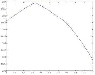
Example 2 – Consider again a symmetric first-price auction with two bidders and sig-nals uniformly distributed in [1.5,3] such that the value of the object is given by v(ti, t−i) =
ti
¡
t−i−t2i
¢
. In Appendix D, we show that this auction does not have monotonic regular equi-libria, but there is a bell-shaped equilibrium as shown in Figure 2.¥
Example 1 shows that it is possible for a standard auction to have multiple equilibria. Example 2 suggests that the correct conjugation can fail to exist – at least with a fixed shape (that we began assuming). Thus, one would be interested in cases where it is possible to ensure the uniqueness of the equilibrium and where it is possible to find explicitly the conjugation. We do this under the context of assumption H3, to be presented in the next subsection.
5. Equilibrium Existence of Weakly Separable Auctions
Theorem 2 teaches us that the question of equilibrium existence is solved if we are able tofind the proper conjugation. In examples 1 and 2 of the previous section we have shown situations where the conjugations could be obtained. However, there we assumed some features of the conjugation that are not necessary and we were able to find the correct conjugation for those settings. Now we will work in a setting where a conjugation always exists: the weakly separable auctions. These are the auctions satisfying the following assumption:
(H3) (Weak Separability). v(ti, t−i) is such that if v(ti, t−i) < v(t0i, t−i) for some t−i then
v¡ti, t0−i
¢
< v¡t0
i, t0−i
¢
for allt0
v1(s)∈C}= 0, where
v1(s)≡E[v(ti, t−i)|ti =s]
is the expected value of the object for bidder with type s.
Assumption (H3) is restrictive, but it is valid in many economic meaningful cases.8 Of course, private values are included in (H3).
Under (H3), we can define explicitly the conjugation: (19) P(ti)≡Pr
©
t−i∈SN−1 :v1(tj)< v1(ti), j6=i
ª
.
Moreover, we can give a necessary and sufficient condition for the equilibrium existence of the direct auction: merely that the solution ˜bto thefirst-order condition of the indirect auction be increasing. This is the content of the following:
Theorem 3 (Necessary and Sufficient Condition For Equilibrium Existence). Assume (H0)-(H3). LetP be defined by (19) and let ˜vbe given by (5) for thisP. There exists an equilibrium b∈S if there exists an increasing function ˜bthat satisfies
(20)
Z y
0
pW³˜b(y),˜b(α)´dα+
Z 1
y
pL³˜b(y),˜b(α)´dα=
Z y
0
˜
v(α,α)dα.
If this is the case, the equilibrium of the direct auction is given byb = ˜b◦P and the expected payment of a bidder of type sis given by
(21) p(s) =
Z P(s)
0
˜
v(α,α)dα.
Additionally, if ˜vis continuous, then there exists an equilibriumb∈Sand there exists∂bΠ(s, b(s))
for all sif and only if there exists an increasing function ˜bthat satisfies the following:
• For (H1)-1, ˜bis differentiable and
˜b0(x) = ˜v(x, x)−p
W³˜b(x),˜b(x)´+pL³˜b(x),˜b(x)´
Eα h
∂1pW ³
˜
b(x),˜b(α)´1[˜b(x)>˜b(α)] +∂1pL ³
˜
b(x),˜b(α)´1[b˜(x)<˜b(α)]
i;
with initial conditionR01pL³˜b(0),˜b(α)´dα= 0;
• For (H1)-2, ˜bis continuous and satisfies, for all x∈(0,1), ˜
v(x, x)−pW³˜b(x),˜b(x)´+pL³˜b(x),˜b(x)´= 0.
Moreover, if there is a unique ˜b that satisfies such properties, the equilibrium of the direct auction in regular pure strategies is also unique.
Proof. See Appendix C.¥
8Theorem 3 of Debreu (1960) implies that ifSis connected andvsatisfies (H3), thenv(t
i, t−i) can be written
ashu1(t
i) +u2(t−i)
, wherehis an increasing function. In this case, (H3) would also imply thatu1(t
i) does
Remark 3. As explained in Remark 1, if a multidimensional auction has a regular equilib-rium, it can always be reduced (in a non-trivial way) to a one dimension auction (the indirect auction). So, for obtaining equilibrium existence, we have to consider auctions that can be “reduced”. This is what assumption H3 allows us to explicitly do. It still encompasses cases where such reduction is not trivial, as we show in examples 3 and 4 below. The reduction of the dimension of types is not a novelty in auction theory. While studying the efficiency of auctions, Dasgupta and Maskin (2000) use a condition close to H3 and Jehiel, Moldovanu and Stacchetti (1996) made such reduction for revenue maximization. Nevertheless, to show equilibrium exis-tence in auctions, one cannot use only H3 or the Dasgupta and Maskin’s condition, since the received theory would require the monotonicity assumption of ˜v on the reparameterized types. As we show in examples 4 and 5, this is not always possible. So, an important feature of Theorem 3 is that it does not require ˜v to be monotonic.
Example 3 (Spectrum Auction).9
Consider afirst-price auction of a spectrum license. The license covers two periods of time: (1) In thefirst period, the regulator lets the winner explore its monopoly power. Lett1i be the estimative of bidder iof the monopolist surplus in this first period. Of course, the true surplus will be better approximated by ¡t11+...+t1N¢/ N. If the bidder i (afirm) wins the auction, it has to invest t2i, a privately known amount, to build the network that will support the service. So, in the first period, the license gives to thefirm
t11+...+t1N N −t
2
i.
(2) In the second period, the regulator makes an estimate of the operational costs of the
firm. The regulator cannot observe the true operational cost, t3i, which is a private information of the firm. Nevertheless, the regulator has a proxy that is a sufficient statistic for the mean operational cost of all participants in the auction, ¡t31+...+t3N¢/ N. The regulator will fix a price that will give zero profit for a firm with the mean operational costs.10 So, in the second period, the license gives to the winner
t31+...+t3N N −t
3
i.
So, the value of the object is given by
v(ti, t−i) =
t11+...+t1N N −t
2
i +
t31+...+t3N N −t
3
i.
Let the signals ti =
¡
t1i, t2i, t3i¢, i= 1, ..., N, be independent. Observe that the problem cannot be reduced to a single dimension. Indeed, if we summarize the private information by, say, si =t1i/N−t2i +t3i(1/N−1), we lose the information about t1i and t3i that are needed for the
value function of biddersj6=i. Also, the model cannot be reparameterized to an increasing one. If we try to put−t3i in the place oft3i, then the dependence ofv(ti, t−i) on the signalst3j will be
decreasing. So, the received theory does not ensure the existence of pure strategy equilibrium for this case. Nevertheless, assumption (H3) is trivially satisfied. In Appendix D, we assume
9This example is more complex, but formally similar to example 5 of Dasgupta and Makin (2000).
10We assume that the regulator is institutionally constrained to follow such a procedure, so the optimality of
the ti =
¡
t1i, t2i, t3i¢are independent and uniformly distributed on £s1, s1¤ × £s2, s2¤ ×£s3, s3¤, with s1, s2, s3 > 0 and we show that a sufficient condition for the existence of equilibrium in pure strategy is
s1 N −s
2−s3N −1
N −1>0.
The derivation in Appendix D indeed provides necessary and sufficient conditions for the exis-tence of equilibrium.¥
Example 4 (Job Market).
We model the job market for a manager as an auction among competing firms, where the object is the job contract. It is natural to assume that the manager has a multidimensional vector of characteristics,m = (m1, ..., mk). For the sake of simplicity, we assume thatfirms learn such
characteristics through interviews and curriculum analysis. Eachfirm also has a position to be
filled by the manager, with specific requirements for each dimension of the characteristics. For instance, if dimension 1 is ability to communicate and the position is to be the manager of a production section, there is level of desirability of this ability. An overly communicative person may not be good. The same goes for the other characteristics. A bank may desire a sufficiently (but not exaggeratedly) high level of risk loving or audacity on the part of the manager, while a family business may desire a much lower level. Even efficiency or qualification can have a level of desirability. Sometimes, the rejection of a candidate is explained by over-qualification. Therefore, letti = (t1i, ..., tKi ) be the value of the characteristics desired by the firm.
Since firms are competitors, then if one hires the employee, the other will remain with a vacant position, at least for a time.11 In this way, the winning firm also benefits from the fact that its competitors have a vacant position – and, then, are not operating perfectly well. The higher the abilities required for the job, the more the competitor suffers.12 So, the utility in this auction is as
v(ti, t−i) = K
X
k=1
akmk−
K
X
k=1
bk³tki −mk´2+X
j6=i K
X
k=1
cktkj,
where ak is the level of importance of characteristic k of the manager, bk > 0 represents how
important is the distance from the desired leveltk
i of the characteristick, and ck is the weight
of the benefit that firm i receives from the fact that the competitors are lacking Pj6=itk j of
the ability k. As in the previous example, we cannot simplify this model to a unidimensional monotonic model. In Appendix D we analyze the case where there is just one dimension (K = 1), 2 players (N = 2) and types are uniformly distributed on [0,1], b=b1 >0. We show that when
11This model works only for non-competitive job markets. In other words, the buyers (the contractingfirms)
have no access to a market with many homogenous employees to hire. This is implicit when we model it as an auction. So, this is the reason why afirm that does not contract the manager suffers – it is not possible tofind a suitable substitute instantaneously.
12Iffirms act in a oligopolistic market, it is possible to justify such externality through the fact that the vacant
0 0.1 0.2 0.3 0.4 0.5 0.6 0.7 0.8 0.9 1 0.02
0.025 0.03 0.035 0.04 0.045 0.05 0.055 0.06 0.065 0.07
Figure 3. Equilibrium bidding function in Example 4.
m1 =m >1/2, there exists a pure strategy equilibrium in regular strategies if and only if
c≡c1 >max
½
2b(m−2)
3 ,
2b(1−2m) (1 +m) 3
¾
and when m <1/2, if and only if
c6min
½
2b(m+ 1)
3 ,
2b(1−2m) (1 +m) 3
¾
.
Observe that for both cases the valuec= 0 ensures the existence of equilibrium. This is expected, since it corresponds to a private value auction. For a =b = 1/5, c = 1/20 and m = 1/3, the equilibrium bidding function is shown in Figure 3.¥
Now, we can return to the example given in the introduction. Theorem 3 gives the conditions for the equilibrium existence.
Example 5 (JSSZ, example 1). Let us consider a first price auction with two bidders, independent types uniformly distributed on [0,1]. Letv1(t
i) =ti and v2(t−i) =α+βt−i. It is
clear that P(ti) =ti in this case and ˜v(x, y) =α+x+βy. So, ˜v(x, x) =α+ (1 +β)x and
˜
b(x) = 1 x
Z x
0
˜
v(z, z)dz = 1 x
·
αx+(1 +β)x
2
2
¸
=α+ (1 +β)x 2 ,
which is increasing only ifβ >−1. Observe that for ˜b(·)>0, it is necessary α>−(1 +β)x/2, otherwise negative bids have to be allowed.¥
Instead, consider the following rule: if a tie occurs, conduct an all-pay auction among the tying bidders. If another tie occurs, split randomly the object.13,14
We show now that the all-pay auction tie-breaking rule ensures the existence of equilibrium for all auctions that we are considering.
Theorem 4 (General Existence). Assume (H0) - (H3) and that the all-pay auction tie-breaking rule is adopted. If there is a continuous function ˜b, not necessarily increasing, such that
Z y
0
pW³˜b(y),˜b(α)´dα+
Z 1
y
pL³˜b(y),˜b(α)´dα=
Z y
0
˜
v(α,α)dα,
then there exists a pure strategy equilibrium.
Proof. See Appendix C.¥
Remark 4. The main ingredients in the proof of Theorem 4 are the payment expression and the fact the bidding function of an all-pay auction is always increasing. This is so because in the all-pay auction, the bid
˜b(x) =Z x
0
˜
v(α,α)dα
is exactly the expect payment, which implies (20). Since v is positive by (H0), ˜v is positive which implies that ˜b is increasing. Thus, an auction that has an increasing ˜b, as the war of attrition, can be also used as the tie-breaking mechanism.
Example 5(cont.) With the all-pay auction tie-breaking rule, the equilibrium of Example 5 is given, if β 6−1, by the bid strategy b1(x) = ¯b,∀x ∈[0,1], in thefirst price auction, where ¯b∈hα+1+β
2 ,α i
, and the bid strategy
b2(x) =αx+1 +β 2 x
2
for the tie-breaking (all-pay) auction.¥
Remark 5. When ˜b is not increasing, there are types that are not ordered correctly (as in Example 5). This can be understood as a failure of ˜bin correctly revealing the information that each bidder possesses. One can say that the tie-breaking rule has exactly the role of revealing information, in this sense. Thus, Theorem 4 can be interpreted as saying that all-pay auctions and war of attrition are better mechanisms for revelating information thanfirst-price and second-price autions. This can be another way of justifying the use of research tournaments in practice.15 Indeed, the characteristics needed to compete for a research is very intricated: it is needed
13Observe that in the tie-breaking auction, bids and payments may be less than in thefirst auction.
14Maskin and Riley (2000) used a similar tie-breaking rule. They propose to conduct a second price (Vickrey)
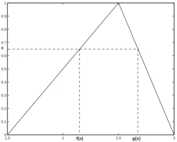
auction in the case of a tie.
ak ck bk
x0 x1 y0 y1 z1
z0
Figure 4. Possible specifications for the level of the tie.
information not only on the technical capabilities, but also on discipline, honesty, creativity, etc. This (multidimensional) information is better revealed through an all-pay auction.16,17
The reader should note that Theorem 4 does not claim the uniqueness of equilibrium. Indeed, if ˜b is not increasing, there are many equilibria. There are two sources for this multiplicity.
Thefirst source is that under the all-pay auction tie-breaking rule, any level of the bid in the range where ˜b is not increasing can be chosen to be the level of the tie. This is shown in the Figure 4. For instance, anya0can be chosen betweenx0 andx1. Once one of the three elements
ak, bk or ck is determined, so are the other two. However, these possibilities lead to the same
expected payment and payofffor each bidder in the auction.
Another point is that the tie-breaking rule is not unique, in general. It can be shown, for instance, that for cases where ˜bis decreasing (as in example 1 of JSSZ) and for some specifications of v, there is a continuum of tie-breaking rules (like that defined by JSSZ for their example 1), which ensures the existence of equilibrium. All these tie-breaking rules nevertheless imply different revenues. In light of this observation, the existence of equilibrium with an endogenous
tie-breaking rule seems even more problematic as a solution concept, since it can sustain many different behaviors and payoffs at equilibrium.
This multiplicity is in contrast with the “ironing principle” usual in Contract Theory.18 The unicity of the solution through the ironing principle comes from a Lagrangian condition that must be satisfied by the contract. Here, we do not have the maximization function of the principal. So, there is no additional condition that wouldfix the level of tieing bids.
16Standard explanations for the use of tournaments in research also appeals to the role of information. See,
for instance, Taylor (1995, p. 872): “Contracting for research is often infeasible because research inputs are unobservable and research outcomes cannot be verified by a court”. Our point is somewhat different, but obviously related to this explanation. The comparison among the information revealed by different auctions is the novelty.
17Obviously, these observations are valid only under the context of assumptions (H0)-(H3). It is a matter for
future research to determine the range of validity of the existence ensured by all-pay auction tie-breaking rule.
The reader may observe that the expression of the payment in Theorem 3 depends only on the conjugation, which is fixed for all kind of auctions. Also, the payment is exactly the same under the all-pay auction tie-breaking rule. So, we have the following:
Theorem 5(Revenue Equivalence Theorem). Consider auctions that satisfy (H0) -(H3) and with the all-pay auction tie-breaking rule. Then, any format of the auction gives the same revenue, provided that bidders follow the symmetric equilibrium specified by Theorem 4.
Proof. See Appendix C.¥
6. Conclusion
Now we will briefly highlight what are the most important contributions of this paper and discuss possible extensions.
6.1. The Contributions. Our contributions can be summarized as follows:
• Equilibrium Existence in the Multidimensional Setting – McAdams (2003a) generalizes Athey (2001) for multidimensional types and actions. He works with discrete bids and continuous types. Our approach gives the existence with continuum types and bids. Our result provides the expressions of the bidding functions, while his is an existence result only. His assumptions require monotonicity and are not on the fundamentals of the model. On the other hand, our results do not cover multi-unit auctions nor asymmetries as his. JSSZ give the existence for multidimensional games, including cases with dependence, while we require independence. However, they need an endogenous tie-breaking rule, and the existence is in mixed strategies, while our results are in pure strategies. Jackson and Swinkels (2004) show the existence of equilibria for a large class of multidimensional private value auctions. Their setting is private values, while ours is interdependent values. They allow asymmetries, dependence of signals and multi-units, but the existence is given in mixed strategies.
• Equilibrium Existence in Non-Monotonic Settings – We are not aware of any general non-monotonic equilibrium existence results in pure strategies. Zheng (2001), Athey and Levin (2001) and Ewerhart and Fieseler (2003) present cases where non-monotonicity arises.
Thus, our method develops a theory to deal with the situations where the usual monotonic-ity is not fulfilled.19 Araujo and Moreira (2000) use a similar method for the screening problem without the single crossing property and Araujo and Moreira (2001) extend it to signaling model.
• Uniqueness of Equilibrium – We are able to ensure the uniqueness of equilibrium in the symmetric interdependent values auctions that satisfy assumption H3, extending the well known uniqueness of unidimensional and monotonic auctions.
19Of course, papers that provide existence in distributional (mixed) strategies can treat non-monotonic settings
• Necessary and Sufficient Conditions for the Existence of Equilibrium without Ties – The results of JSSZ do not allow one to distinguish when special tie-breaking is needed or when it is not. Our approach clarifies, under assumption H3, whether ties occur with positive probability (and there is a potential need for special tie-breaking rules).
• All-Pay Auction Tie-Breaking Rule – When there is a need for a tie with positive probability, we are able to offer an exogenous tie-breaking rule, which is implemented through an all-pay auction. Moreover, the equilibrium that the rule implements is in pure strategies. For private value auctions, Jackson and Swinkels (2004) show that the equilibrium is invariant for any trade-maximizing tie-breaking rule. Nevertheless, this does not need to hold for the interdependent values auctions that we treat here.
• Information Revelation – In the sense made precise by Remark 5, we show that all-pay auction and war of attrition are better mechanisms to reveal information thanfirst-price and second-price auctions.
• Revenue Equivalence Theorem – We have also generalized the Revenue Equivalence Theorem (Theorem 5). Furthermore, Theorem 2 and Appendix B show that there is a deep connection between the revenue equivalence and the existence of equilibrium. Riley and Samuelson (1981) and Myerson (1981) establish that revenue equivalence is a consequence of the equilibrium behavior. Proposition 5 and Corollary 1 in Appendix B show that the revenue equivalence is also sufficient for the existence of equilibrium (if an extra condition is satisfied).
Thus, our results have clarified some aspects of the equilibrium existence problem in auctions. The theory shows that, under assumption H3, there is no additional difficult in working with the more general setting of multidimensional types and non-monotonic utilities besides those difficulties already present in the unidimensional setting.20 Moreover, this approach allows the equilibrium bidding functions to be expressed in a simple manner. This is so because the equilibrium bidding function of a general auction can be expressed by the equilibrium bidding function of an auction with two bidders and types uniformly distributed on [0,1].
6.2. Limitations of the Method. Our theory makes two important assumptions: indepen-dence of the types and symmetry.
The generalization of this approach for dependent types involves some difficulties, because the conjugation would depend in a complicated way on types. Nevertheless, we believe that some extension can be done if we assume conditional independence.21 It is worth remembering that the problem with dependence is not specific to our approach. Jackson (1999) gives a counter-example for the equilibrium existence of an auction with bidimensional affiliated types. Fang and Morris (2003) also obtain negative results, not only for the existence of equilibrium but also for the revenue equivalence.
On the other hand, asymmetry does not seem to impose severe restriction on the existence of equilibrium. We believe that the approach of the indirect auction can be adapted to this case,
20Theorem 3 shows that the non-existence of the equilibrium comes from the non-monotonicity of the
in-direct bidding function. This can also occur in an unidimensional setting, although it can be more usual in multidimensional models.
although not in a straightforward way. If this can be done, it is unlikely that we will obtain simple expressions as in this paper.
Another limitation of our theory is that it is applied only to single-unit auctions. The risk neutrality does not seem to be a fundamental assumption, although complications can arise in extending the approach for risk aversion.
Finally, the relaxation of assumption H3 is an obvious direction to pursue, although H3 seems to encompass many important economical examples.
Appendix A - Proof of the Basic Results
We will need the following result, which was proved, in a more general setting, by de Castro (2004a).
Lemma 1 (Payoff Characterization)– Assume (H0)-(H2). Fixb(·)∈S. The bidderi’s payoffcan be expressed by
Π(ti, bi, b(·)) =Πi(ti, bmin) + Z
(bmin,bi)
∂biΠ(ti,β, b(·))dβ,
where∂biΠ(ti,β, b(·)) exists for almost all β with
∂biΠ(ti,β, b(·)) =E
h −∂1pW
¡
β, b(−i)(t−i)
¢
1[β>b(−i)(t−i)]−∂1p
L¡β, b
(−i)(t−i)
¢
1[β<b(−i)(t−i)]
i
+E[v(ti, t−i)−pW (β,β) +pL(β,β)|b(−i)(t−i) =β]fb(−i)(β).
a.e., where b(−i)(t−i)≡maxj6=ib(tj).
Proof. Let us define b(−i)(t−i) ≡ maxj6=ib(tj). Since bi =b(−i)(t−i) with probability zero,
we have
Π(ti, bi, b(·)) =
Z
SN−1 £
v(ti, t−i)−pW
¡
bi, b(−i)(t−i)
¢¤
1[bi>b(−i)(t−i)]
Y
j6=i
µ(dtj)
+
Z
SN−1
£
−pL¡bi, b(−i)(t−i)
¢¤
1[bi<b(−i)(t−i)]
Y
j6=i
µ(dtj).
Take a sequence an → b−i , i.e., an < bi (the other case is analogous). We want to prove that
there exists limn→∞Dn(bi)/(bi−an) for almost all bi, where
In the sequel, we will omit the measureQj6=iµ(dtj) and the termst−i. We have:
Dn(bi) =
Z £
v(ti,·)−pW
¡
bi, b(−i)(·) ¢¤
1[bi>b(−i)(·)]1[an>b(−i)(·)]
+Z £−pL¡bi, b(−i)(·) ¢¤
1[bi<b(−i)(·)]
−Z £v(ti,·)−pW
¡
an, b(−i)(·) ¢¤
−Z £−pL¡an, b(−i)(·) ¢¤
1[an<b(−i)(·)]
= Z £v(ti,·)−pW
¡
bi, b(−i)(·) ¢
+pL¡an, b(−i)(·) ¢¤
1[bi>b(−i)(·)>an]
+Z £−pW¡bi, b(−i)(·) ¢
+pW¡an, b(−i)(·) ¢¤
1[an>b(−i)(·)]
+Z £−pL¡bi, b(−i)(·) ¢
+pL¡an, b(−i)(·) ¢¤
1[bi<b(−i)(·)]
Let us call the three last integrals asD1
n(bi),D2n(bi) andDn3(bi), respectively. SincepW and
pL are differentiable, we have
lim
n→∞
D2n(bi)
bi−an
= − lim
n→∞
Z pW¡a
n, b(−i)(·) ¢
−pW ¡b
i, b(−i)(·) ¢
bi−an 1[bi>b(−i)(·)]
= − Z
∂1pW ¡
bi, b(−i)(·) ¢
1[bi>b(−i)(·)]
and
lim
n→∞
D3n(bi)
bi−an
= − lim
n→∞
Z pL¡a
n, b(−i)(·) ¢
−pL¡b
i, b(−i)(·) ¢
bi−an 1[an<b(−i)(·)]
= −
Z
∂1pL¡bi, b(−i)(·) ¢
1[bi<b(−i)(·)].
everywhere. So, if we put a0 =bmin and bi>bmin, the Fundamental Theorem of Calculus gives
(22) D20(bi) =
Z
(bmin,bi)
Z
−∂1pW ¡
α, b(−i)(·) ¢
1[bi>b(−i)(·)]dα
and
(23) D03(bi) =
Z
(bmin,bi)
Z
−∂1pL¡α, b(−i)(·) ¢
1[bi<b(−i)(·)]dα.
Now, define the measure ρoverR+ by ρ(V)≡
Z
SN−1 £
v(ti, t−i)−pW
¡
bi, b(−i)(t−i)
¢
+pL¡bi, b(−i)(t−i)
¢¤
1[b(−i)(t−i)∈V]
Y
j6=i
µ(dtj) .
Observe that, since b∈S,ρis absolutely continuous with respect the Lebesgue measureλ. We have
lim
n→∞
Dn1(bi)
bi−an
= lim
n→∞
ρ([an, bi))
bi−an
= lim
an
→bi
½
ρ([an, bi))
λ([an, bi))
¾
where ddλρ(.) is the Radon-Nikodym derivative of ρ with respect to λ. Indeed, the existence of such limit is ensured by Theorem 8.6 of Rudin (1966) for almost allbi, that is,
λ µ½
bi :@ lim an
→bi
½
ρ([an, bi))
λ([an, bi))
¾¾
= 0.
It is easy to see that the Radon-Nikodym derivative ddλρ(bi) is simply
E[v(ti, t−i)−pW(β,β) +pL(β,β)|b(−i)(t−i) =β]fb(−i)(β),
wherefb(−i)(β) is the Radon-Nikodym derivative of the distribution of maximum bids, R
1[b(−i)(t−i)∈V].
Moreover, Theorem 8.6 of Rudin says that
(24) ρ((bmin, bi)) =
Z
(bmin,bi)
dρ
dλ(α)dα.
Thus, (22), (23) and (24) imply that
Π(ti, bi, b(·)) =Π(ti, bmin) + Z
(bmin,bi)
∂biΠ(ti,β, b(·))dβ,
where
∂biΠ(ti,β, b(·)) =E
h
−∂1pW¡β, b(−i)(t−i)
¢
1[β>b(−i)(t−i)]−∂1p
L¡β, b
(−i)(t−i)
¢
1[β<b(−i)(t−i)]
i
+E[v(ti, t−i)−pW(β,β) +pL(β,β)|max
j6=i b(tj) =β]fb(−i)(β).
This concludes the proof.¥
Proof of Proposition 1. Let us introduce the following notation: Π+(ti, c) =
Z £
v(ti,·)−pW
¡
c, b(−i)(·) ¢¤
1[c>b(−i)(·)]Πj6=iµ(dtj)
Π−(ti, c) =
Z
pL¡c, b(−i)(·) ¢
1[c<b(−i)(·)]Πj6=iµ(dtj),
˜
Π+,−(φi, c)≡EhΠi+,−(ti, c)|P(ti) =φi
i
.
Let us begin with the proof for ˜Π+i and Π+i . Let us denote the conditional expectation by
(25) gti,c
(α)≡Ehv(ti, t−i)−pW
¡
c, b(−i)(t−i)
¢
|P(b−i)(t−i) =α
i
.
The event £c > b(−i)(t−i)
¤
occurs if and only ifhP˜b(c)> Pb
(−i)(t−i) i
occurs. Then, we have
Π+(ti, c) =
Z
gti,c³
P(b−i)(t−i)
´
1˜
Pb
(c)>Pb
(−i)(t−i)
Πj6=iµ(dtj).
Now we appeal to Lemma 2.2, p. 43, of Lehmann (1959). This lemma says the following: if R is a transformation and ifµ∗(B) =µ¡R−1(B)¢, then
Z
R−1(B)
g[R(t)]µ(dt) =
Z
B
In our case, R= Pb
(−i) and µ∗([0, c]) =µ∗([0, c)) = τ−i ³¡
Pb¢−1
(−i)([0, c)) ´
= Pr{t−i ∈ SN−1 :
Pb(t
j)< c}= c, by (4). So,µ∗ is exactly the Lebesgue measure, and we have
(26) Π+(ti, c) =
Z P˜b
(c)
0
gti,c
(α)dα.
From this and the definition of ˜Π+, we have
˜
Π+(φi, c) =E
"Z P˜b
(c)
0
gti,c
(α)dα|Pb(ti) =φi
#
=
Z P˜b
(c)
0
Ehgti,c
(α)|Pb(ti) =φi
i
dα
=
Z P˜b
(c)
0 h
˜
v(φi,α)−pW ³c,˜b(α)´idα,
where the second line comes from a interchange of integrals (Fubbini’s Theorem) and the last line comes from independency and the definition of ˜v(φi,α) andgti,c(α) (see (5) and (25)). Also
from the fact that ˜b=³P˜b´−1, we can substitute ˜Pb to obtain
(27) Π˜+(φi, c) =
Z ˜b−1(c)
0 h
˜
v(φi,α)−pW³c,˜b(α)´idα.
Now, we can repeat the above procedures with Π−(φi, c) and obtain:
(28) Π˜−(φi, c) =
Z 1
˜
b−1(c)
pL³c,˜b(α)´dα.
Adding up, that is, putting ˜Π(φi, c) = ˜Π+(φ
i, c)−Π˜−(φi, c), we obtain the interim payoffof
the indirect auction. This concludes the proof of the first part.
For the second part, observe that the equality (8) implies that for all ti such that Pb(ti) =
Pb(s) =x,
Ehgti,c
(α)|Pb(ti) =x
i
=Eh¡v(ti, t−i)−pW
¡
c, b(−i)(t−i)
¢¢
|Pb(ti) =x, P(b−i)(t−i) =α
i
=Eh¡v(ti, t−i)−pW
¡
c, b(−i)(t−i)
¢¢
|ti =s, P(b−i)(t−i) =α
i
=Eh¡v(s, t−i)−pW
¡
c, b(−i)(t−i)
¢¢
|P(b−i)(t−i) =α
i
Then,
˜
Π+(x, c) =E
"Z P˜(c)
0
gti,c
(α)dα|Pb(ti) =x
#
=
Z P˜(c)
0
Ehgti,c
(α)|Pb(ti) =x
i
dα
=
Z P˜(c)
0
gs,c(α)dα
=Π+(s, c),
where the last line comes from (26). Obviously, the same can be done forΠ− and ˜Π−. So, the proof is complete.¥
Appendix B - Indirect Auction Equilibria
In this appendix, we will analyze auctions between two players, with independent types uni-formly distributed on [0,1]. Since this is the setting of the indirect auction, we will use notation consistent with that, although the results of this appendix are independent from the results of section 4. For (i,−i) = (1,2) or (2,1) let
˜
ui(x, b) =
˜
v(xi, x−i)−pW(bi, b−i), ifbi> b−i
−pL(b
i, b−i), ifbi< b−i
˜
v(xi,x−i)−bi
2 , ifbi=b−i
be the ex-post payoff. We will assume:
(H0)’ The types are independent and uniformly distributed on [0,1]. ˜vis positive, measurable and bounded above.
By the definition of the indirect auction, we are interested only in non-decreasing equilibria ˜b, strictly increasing in the range of winning types. That is, for a non-decreasing strategy ˜b, define x0 to be the minimum type that bids at least bmin. So we require ˜b to be increasing in
[x0,1] and equal to ˜b(x) = −1 for x < x0. In order to be an equilibrium, ˜b must satisfy the
following:
(29)
Z x0
0 h
˜
v(x0,α)−pW ³
˜b(x
0),˜b(α) ´i
dα− Z 1
x0
pL³˜b(x0),˜b(α) ´
dα= 0.
Indeed, the above integral is the payoffof x0. If it is negative, thenx0 can do better by bidding −1. If the above integral is positive, thenx0>0, otherwise the payoffofx0 = 0 would reduce to −Rx10p
L³˜b(x
0),˜b(α) ´
dα which is non-positive because pL is positive. If x
0 >0, for ax < x0
sufficiently close of x0, the payoff Z x0
0 h
˜
v(x,α)−pW ³b˜(x0),˜b(α) ´i
dα− Z 1
x0
pL³˜b(x0),˜b(α) ´
is still positive (because of the continuity of ˜v). So,xis receiving zero but could obtain a strictly positive payoffby bidding ˜b(x0) =bmin.
So, for afixed ˜b, we assume the following:
(H2)’ There existsx0, the mininum indirect type that satisfies (29) and x0 ∈[0,1).
We have the following:
Proposition 2(Case 1). Assume (H0)’, (H1)-1, that is, ∂1pW(·) >0 or∂1pL(·) >0, (H2)’
and that ˜v is continuous. Let ˜b be an increasing equilibrium of the indirect auction. Then, ˜bis differentiable and satisfies
(30) ˜b0(x) =
˜
v(x, x)−pW³˜b(x),˜b(x)´+pL³˜b(x),˜b(x)´
Eα h
∂1pW³˜b(x),˜b(α)´
1[˜b(x)>˜b(α)] +∂1pL ³
˜
b(x),˜b(α)´1[b˜(x)<˜b(α)] i.
Proof. The proof is an adaptation of part of the proof of Theorem 2 of Maskin and Riley (1984).22 Suppose that player −i follows ˜b. The interim payoff of player iwith (indirect) type xi is
˜
Π(xi, bi,˜b(·)) =
Z £
˜
v(xi, x−i)−pW(bi, b(x−i))
¤
1[bi>˜b(x−i)]dx−i
− Z
pL(bi, b(x−i)) 1[bi<˜b(x−i)]dx−i.
If ˜b is discontinuous, there exists x∗ >x0, with
lim sup
x<x∗
˜b(x)<lim inf
x>x∗˜b(x).
Consider bidders x+i ε that bids β+ε = ˜b¡x+iε¢= lim infx>x∗˜b(x) +εand x−i ε that bids β−ε =
˜b¡x−ε
i
¢
= lim supx<x∗˜b(x)−ε. We will prove that, for ε > 0 sufficiently small, the bid β−ε
is better than β+ε for a bidder with type x+i ε. This will be the contradiction. The event
h
β+ε>˜b(x−i)
i
is arbitrarily close to hβ−ε>˜b(x−i)
i
. So, the difference of expected utilities
Z
˜
v(x+i ε, x−i)1[β+ε>˜b(x
−i)]dx−i−
Z
˜
v(x+i ε, x−i)1[β−ε>˜b(x
−i)]dx−i
=
Z
˜
v(x+i ε, x−i)1[β+ε>b˜(x−i)≥β−ε]dx−i
is arbitrarily small. On the other hand, the difference of expected payments is