1
In
tergenera
t
iona
l
Transm
iss
ion
of
Educa
t
ion
:
Ev
idence
from
Ind
ia
Teresa
Mar
ia
Tavares
Mora
is
Sarmen
to
1
D
isser
ta
t
ion
wr
i
t
ten
under
the
superv
is
ion
of
Prof
.
Hugo
Re
is
D
isser
ta
t
ion
subm
i
t
ted
in
par
t
ia
l
fu
lf
i
lmen
t
of
requ
iremen
ts
for
the
MSc
in
Econom
ics
,
a
t
the
Un
ivers
idade
Ca
tó
l
ica
Por
tuguesa
,
01
/06
/2018
.
1I wouldliketothank everyonethat helped me duringthe course ofthis work project. First, I wouldliketothank ProfessorHugo Reis forthe guidance, support and availability inthis project. Second, I wouldliketothank my colleagues and friends fortheir helpful comments and words of motivation.
Finally, I wouldliketo deeplythank my family, specially my mother Margarida and my brother Tiago, for allthey have done for me. Tothem I dedicatethis work.
2
Intergenerational Transmission of
Education: Evidence from India
Teresa Maria Tavares Morais Sarmento
Abstract
India is one of the fastest growing economies in the world presenting at the same time significant levels of inequality, in particular in terms of education. Arguably, one of the main issues regarding India´s potential economic development and growth is the lack of skilled labour force. This thesis tackles this constraint in growth by studying how education is transmitted between generations in India.Census data from 1983 to 2009 is utilised to provide empirical evidence to both intergenerational education transmission, as well as to potential mechanisms behind the estimated transmission. Empirical evidence provides three results. Firstly, intergenerational mobility in India has increased, due to an increase in the educational attainment of children of low-educated parents. Secondly, the gender gap is closing in terms of mobility. Thirdly, positive association between increasing mobility and economic performance and education policy.
KEYWORDS: Intergenerational Mobility, Inequality, Education, Education Policy, Gender,
3
Transmissão Intergeracional da
Educação: Dados para a India
Teresa Maria Tavares Morais Sarmento
Abstracto
A Índia é uma das economias com mais rápido crescimento económico do mundo, apresentando, ao mesmo tempo, significantes níveis de desigualdade. Uma das principais particularidades à cerca do potencial de desenvolvimento económico e crescimento da Índia é a falta de força de trabalho qualificada. Esta tese aborda a restrição no crescimento económico através da análise da transmissão de educação entre gerações na Índia. Neste trabalho, são utilizados dados de censos entre 1983 e 2009 de modo a obter evidência empírica sobre a transmissão da educação intergeracional, bem como sobre possíveis mecanismos na origem da mobilidade estimada. As provas empíricas permitem inferir 3 conclusões. Em primeiro lugar, o aumento na mobilidade intergeracional na Índia deveu-se a um aumento no nível educacional de crianças filhas de pais com reduzido nível educacional. Em segundo, as diferenças de mobilidade entre géneros vão diminuindo ao longo dos anos até ao seu desaparecimento. E, finalmente, em terceiro lugar, demonstrou-se uma associação entre o aumento da mobilidade e o desempenho económico e a política educacional.
KEYWORDS: Mobilidade Intergeracional, Desigualdade, Educação, Política Educativa,
4 Index 1. Introduction………....5 2. Literature Review………...6 3. Data………....9 3.1. Sample………....9 3.2. Measurement of Education………...10 3.3. Descriptive Statistics………....10 3.3.1. Educational Variable……….10 3.3.2. Gender………11
3.3.3. Other Control Variables……….11
4. Methodology………11
4.1. Regression Coefficient and Correlation………11
4.1.1. Unconditional Analysis……….….11
4.1.2. Conditional Analysis……….….12
4.2.Transition Probabilities………...…...13
5. Results………...13
5.1. Unconditional Regression and Transition Probabilities………....13
5.1.1. Analysis by Survey Year………14
5.1.2. Analysis by Birth Cohort………14
5.2. Conditional Regression Results……….15
5.3. Gender Gap………15
5.4. Macroeconomic and Institutional Association Factors……….….16
5.4.1. Macroeconomic Association Factors………..17
5.4.2. Institutional Association Factors……….17
6. Conclusion……….19
7. References……….19
8. Tables & Figures………...22
5
1. Introduction
Studying intergenerational mobility in education is important and interesting for two main reasons. On the one hand, endogenous-growth models show that education has a beneficial impact on long-run economic growth, as a part of human capital, through improvement of skills. This, in turn, has positive effects on technology and knowledge that will reflect on productivity. Hence, research on education and its transmission is essential in order to conduct policy that will, in fact, increase human capital in the long-run. On the other hand, intergenerational mobility captures the probability of a child reaching a higher socio-economic status than their parents. Being inequality one of the most studied topics in economics, as well as a crucial concern for policy makers; intergenerational persistency of this inequality (and its causes) are of great interest.
Furthermore, equality of opportunity –where children of disadvantaged backgrounds have the same opportunities as wealthier children - is fundamental, not only for economists, but also for society, as a development goal of its own right. Chevalier et al. (2003), show that people with more educated parents have a higher likelihood to be more educated themselves. The opposite applies for people with less educated parents. This is extremely significant in the sense that less mobility suggests lack of equality of opportunities in the education system.
India is one of the fastest growing economies in the world, and presents high levels of inequality based on a still caste stratified society (although weakened by government measures), which influences low mobility and outcomes (Azam&Bhatt, 2012). In addition, according to OECD’s India Policy Brief in 2014 one of India’s biggest issue is the lack of skills of its labour force. Thus, to improve this situation further research on education is necessary, despite the difficulties provided by the lack of reliable data.
The main goal of this thesis is to study the trend in intergenerational mobility in education in India. Using microdata from several household surveys for the years 1983,1987, 1993, 1999, 2004 and 2009, a series of indexes to measure intergenerational mobility in education will be computed. This paper provides a 30-year estimation for the existing correlations between parents’ and children’s education. Additionally, some of these indexes will provide the direction of the mobility providing values for upward/downward mobility and top/bottom persistence, which, specifically, has not yet been done for the case of India. Considering that in India social, cultural and institutional influence men and women’s educational attainment differently, trends will be described taking into account gender heterogeneity (using different
6
data pairs for males and females). Moreover, so as to contextualize the main results, an analysis for the association between macroeconomic and institutional factors will be presented.
Until now, most research on education intergenerational mobility has been done for North America and Europe, partly due to poor databases (Black & Devereux, 2011). As such, this paper will contribute to widening the research on developing countries. And, although this topic has been already studied for India, this thesis presents a longer time-period span. In addition, for the first time, direction of mobility is provided, as well as the usage of different data pairs for males and females.
This paper is structured as follows. Section 2 provides a literature review on intergenerational mobility. Section 3 explores the details on the data source, sample selection and descriptive statistics. Section 4 is composed by the applied methodology. Section 5 shows the findings for all the estimates using the several indexes and data pairs. Finally, it includes the analysis of association of economic performance and institutions featuring the results obtained.
2. Literature Review
Becker & Tomes (1979) advanced some of the first causality theory models for intergenerational mobility. By developing a model where a family’s utility depends on their own consumption, quantity and quality of children, they broke new ground with both an economic and social approach on inequality and intergenerational mobility theory. Being the quality of the children measured by their adult income. They showed that the biggest the “degree of inheritability and propensity to invest” is, the higher the impact of the family background on children’s well-being.
Later on, Solon (1992) and Zimmerman (1992), measured the degree to which there’s a transmission of family endowments to the next generation, performing estimations for long-term intergenerational income correlation between parents and their children in the US. Using father-son data from the Panel Study of Income Dynamics (Solon) and from the National
Longitudinal Survey (Zimmerman). Both accounted for a smaller degree of mobility compared
to previous research. As well as, demonstrated how earlier work was using biased data and improved measurement method in order to get more robust estimates.
Subsequently, Solon (2004) also focused his work on causality of intergenerational mobility. Starting by extending Becker and Tomes’ (1979) model, he allowed for public investment in human capital. Solon then, concluded that intergenerational mobility elasticity increases
7
parents’ income and education, efficiency of human capital and the returns to its investment, however decrease with the progressivity of government’s investment. Additionally, he stated that the reasons for differences across countries have to do with disparities in the family’s influence, the labour market and the polices that influence a child’s life chances.
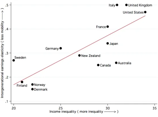
More recently, Corak (2013), using Alan Krueger’s “The Great Gatsby Curve”2 (plots
intergenerational earnings elasticity against inequality measured by the Gini coefficient (see Figure 1)), on a cross-country analysis, shows that countries with higher levels of inequality in income are inclined to present lower levels of mobility. Intergenerational mobility of earnings appears to be much smaller in countries with higher inequality, and higher in countries with more income redistributive policies. Even though, this does not represent a causal relationship, it should not be dismissed. In addition to, intergenerational income mobility, we can also study the intergenerational transmission of education, which gives us a good perception of an individual’s socioeconomic status.
Measuring intergenerational mobility in education has some advantages over measuring it through income due to: life-cycle bias issue (normally people in their mid-twenties have already finished their education); the non-employment obstacle and measurement trouble (people can tell you most accurately their educational attainment) (Black & Devereux, 2011). Estimates by country and over time have been mostly only done for European and North American countries. Until now, the most complete work, for cross-country analysis, is the paper by Hertz et al. (2007), where they give us a 50-year trend of the intergenerational persistence for a sample of 42 countries. The countries that accounted for the biggest persistence were the Latin American countries, which correlation between children and parent schooling accounted for 0.6. While the correlation for the US accounted for 0.46, followed by Western Europe that accounted for 0.4. The Nordic countries presented the highest level of mobility. Furthermore, Neidhöfer, Serrano and Gasparini (2017), give estimates for a series of measurement mobility indexes for the 18 countries of Latin America, for the last 50 years, using the Latinobarometro survey (waves from 1998-2015) that included retrospective questions on parental education. They found that mobility has been increasing over time and mainly due to the increase in upward mobility of children that come from low educated parents.
2On Krueger’s speech, “The Rise and Consequences of Inequality,” to the Center for
8
Moreover, they relate the differences between countries with income inequality, poverty, economic growth, public educational expenditures and assortative mating.
For research on India we have, Jalan and Murgai’s (2008) work, where they investigate education intergenerational mobility using the 1992-93 and 1998-99 National Family Health
Surveys (NFHS), for adults between 15-19 years old. Giving emphasis to the social class and
caste. Their main results are that intergenerational mobility in education had been increasing considerably. Compared to other countries, India showed to have average or even above average mobility estimates. Additionally, they found evidence of inequality of opportunities between castes and social groups, that, when controlled for other factors, the education gap is not that relevant.
In Azam and Bhatt’s (2012) paper, they used the 2005 India Human Development Survey (IHDS), from where they were able to collect a father-son data set (father’s education for almost every male adult respondent between 20-65 years old). One significant difference between this paper and Jalan and Murgai’s (2008) is that Azam and Bhatt (2012) do not rely on the co-residence condition to get the father-son data which would result in a considerable loss of observations. Although, this is only possible because in the IHDS the respondent is asked directly about parents’ education, whilst in the NFHS there is only access to parents’ education from the individuals that live with their parents. By estimating education intergenerational mobility correlation, they show how India ranks compared to the rest of the world’s estimates. Besides that, they obtain results for data across Indian states and social groups. They accounted for an increase in intergenerational mobility of educational attainment between the two generations at aggregate level and amongst the different social groups and Indian states. There is also, Hnatkovskay, Lahiriy and Pauly’s (2012) work where they study intergenerational mobility, for both income and education in India using different year waves of the National Sample Survey. Focusing their analysis on the differences between scheduled castes and tribes (SC/ST) and non-SC/ST, they show that the differences in intergenerational mobility in income and education between the two groups has been decreasing. Along with these findings, it is shown that SC/ST groups have been choosing different occupations than their parents and this “switch rate” has cached up with the non-SC/ST rate. Hence, concluding that the historical barriers to these groups have been broken.
All things considered, this paper provides a new take on India’s intergenerational mobility in education in the sense that, here, for the first time, the direction of the existing mobility will be
9
presented (bottom/downward and persistence at top). Secondly, an analysis of the different traces between mother/father’s influence on son/daughter’s education will be incurred.
3. Data
The data used in this paper was extracted from the Integrated Public Use Microdata Series (IPUMS), of the Minnesota Population Center. The information on parent and children’s educational attainment through the years was taken from the Socio-Economic Survey,
Household Schedule 10: Employment and Unemployment using the available 6 different year
waves (1983, 1987, 1993, 1999, 2004 and 2009). These were collected and organized by the Ministry of Statistics and Programme Implementation of the Indian Government.
These census focus on characteristics of sample household and household members. They include questions on the educational attainment of all household individuals. Nevertheless, they did not comprise retrospective questions on parents’ education, meaning we only have access to parents’ educational attainment through co-residency of parents and children.
3.1. Sample
These census’ samples are representative of the whole population. Although, due to their nature, it was not possible to use all these observations, since some of them were missing indispensable information to this study. Thus, a sample selection had to be performed for every wave.3 At first, all observations belonging to respondents younger than 23 years old were
excluded in order to allow for tertiary education to be completed. On a second stage, there is the need to guarantee that we have information on the respondent’s and their parents’ educational attainment. Hence, observations that did not have information on these were eliminated (discard the ones that report both mother and father information missing). Afterwards, there were still some observations that did not have information on the respondents’ age and these were dropped. Finally, to guarantee that the younger individuals are, indeed, finished with their education, observations from individuals that reported that are still attending school were dismissed. After removing all the observations, on average, we got a total of 284,087 observations. As a result of this survey not including retrospective questions on parents’ education, there is only access to parents’ education information through co-residency condition. Consequently, a certain loss of observations is detected by excluding
3 See Table A1, in Appendix A.
10
observations for which we do not know the mother or father’s education. These are the missing observations as a result of parents not living in the same household as their children.4
Considering that the first and the last survey are from 1983 and 2009, together with the fact that the respondents are between 23 and 60, we have that the years of birth of the respondents are from 1923 to 1986. For simplicity, the data was divided into 5-year birth cohorts, (1920-1925, 1925-1930, …, 1985-1990). Therefore, we end up with 14 birth cohort classes. By observing Table 1, it is visible that the youngest individuals are the most represented on these samples. Ending up with a downward biased sample. Henceforth, to guarantee that we have more robust estimates, estimations will only be made for cohorts between 1945-1950 and 1980-1985.
3.2. Measurement of Education
Educational attainment was recoded using the number of years of the highest level of education achieved. In a way to get the right number of years to the level of education, this recoding follows the Indian education system. Being 0 years of schooling corresponding to “no schooling” and 15 years corresponding to “university completed” (See Table 2). In terms of the parents’ educational attainment, this will be defined as the average of both of the parents. Observations that had information on one of the parents’ missing were reported has a single parent value.5
3.3. Descriptive Statistics 3.3.1. Educational Variable
Tables 3 and 4 depict the average and standard deviation of the years of schooling for both parents and children per birth cohort of the child and survey year. Firstly, its shown that the average years of schooling is higher for children than for parents which is an indicator of increasing education, in general, in India through the years. And if education is expanding in general, it also makes sense the increasing standard deviation. Additionally, we can also observe that average education increases, for both parents and children, has the years of the survey go by: in 1983 we have, on average, for parents 0.97 years of education, while in 2009 we have, on average, 2.68 years of education; and for children we have 4.24 years of education,
4 SeeAppendix B for alternative sample selection.
5In literature is also common to use only the father’s educational attainment or using the highest level
11
on average, in 1983 and for 2009 we have, on average, 8.49. Moreover, it is visible that, for every single year of the surveys, there is a rise in average years of schooling, for both parents and children, as the birth cohorts go by, again pointing out for a general higher level of schooling through time.
3.3.2. Gender
Table 5 depicts the number of observations by gender, for both parents and children. For parents, we have information on mother education, on average, for 90% of the total number of observations, and on father education for 67% of the observations. It can also be observed that most of the respondents of the surveys were males, on average 88%, meaning that sons are more represented than daughters on these samples.
The trend of increasing average and standard deviation of years of schooling as years go by and has birth cohorts go by, is present for both mother and father. In comparison with each other, mothers present lower levels for average and standard deviation as fathers (See Tables 6 and 7).
Again, both daughters and sons present rising average and standard deviation of years of schooling as years and birth cohorts go by. On a first stage, sons present higher levels of education compared to daughters, however, girls start catching up, even reaching higher levels of schooling than boys for the last survey year for the two youngest birth cohorts (See Tables 8 and 9).
3.3.3. Other Control Variables
Controls for individual characteristics that may influence educational attainment were added to the original regression in order to find out to what extent the parameter measuring parental education is driven by other factors.6
4. Methodology
Following the literature, in order to measure intergenerational mobility 5 different mobility indexes will be computed:
4.1. Regression Coefficient and Correlation 4.1.1. Unconditional Analysis
12
The most common way in literature to measure intergenerational mobility is to estimate the intergenerational elasticity (β) which is estimated by regressing child’s education level (𝐸𝑐) on
parent’s education level (𝐸𝑝):
𝐸𝑖𝑐 = 𝛼 + 𝛽𝐸𝑖𝑝+ 𝜀𝑖
In this regression, α is a constant, 𝐸𝑖𝑐is the children’s educational attainment in years, 𝐸𝑖
𝑝 is the
educational attainment in years for every individual 𝑖. β is a measure of persistence, since it represents the rise in children’s education in years of schooling if the parents’ education increases 1 year of schooling (meaning that 1- β is the mobility measure). In addition, in order to take into account, the differences in the distributions of children’s and parents’ education the β is taken as a standardized index:
𝑟 = 𝛽 𝜎𝑖
𝑝
𝜎𝑖𝑐
Where 𝜎𝑖𝑝and 𝜎
𝑖𝑐 are the standard deviations of both parents’ and children’s education
respectively. r also represents a measure of persistence (meaning 1-r is the mobility measure). The β and r represent structural and exchange mobility, correspondingly. Structural mobility comes from the change in the shapes of the marginal distributions, for example an expansion of the average years of schooling, while exchange mobility refers to the exchange of individuals between positions (Jänti and Jenkins, 2013).
Different regressions will be calculated for every 5-year birth cohort, in order to get estimations for the individuals born in each period. They will also be calculated for each survey year. Doing this instead of using the same regression for all the birth cohorts and years, besides of giving us a trend for the last 30 years, has the advantage of not giving more weight to the cohorts that have more observations, this way the cohort effects are being captured. Hence, this will correct for the fact that the oldest cohorts are smaller and for the fact that older cohort shares may differ from population shares (Hertz et al., 2007).
4.1.2. Conditional Analysis
As stated in section 3, control variables were included to the regression utilized to calculate the beta index.
First, age was added considering that education is expected to increase with age. The dummy
13
value 1 if the respondent is female and 0 if the respondent is male. Furthermore, there were present in the data big disparities in average schooling between rural and urban households henceforth, the dummy urban is included where it takes the value 1 if the respondent assumes urban status or 0 if the respondent assumes rural status. Finally, there is the need to incorporate the effect of the household type as a control. There are 4 different types of households, thus, three dummys for the different types of households are set (only 3 to avoid dummy trap).
Married which is 1 if the household type is composed by a married couple/couple with children
and 0 otherwise; single which is 1 if the household is a single-parent family and 0 otherwise;
relatives which is 1 if household type composed by extended family and 0 otherwise7. By
adding these controls, we get the following regression:
𝐸𝑖𝑐 = 𝛼 + 𝛽𝐸𝑖𝑝+ 𝑎𝑔𝑒𝑖 + 𝑓𝑒𝑚𝑎𝑙𝑒𝑖 + 𝑢𝑟𝑏𝑎𝑛𝑖 + 𝑚𝑎𝑟𝑟𝑖𝑒𝑑𝑖+ 𝑠𝑖𝑛𝑔𝑙𝑒𝑖 + 𝑟𝑒𝑙𝑎𝑡𝑖𝑣𝑒𝑖+ 𝜀𝑖
4.2. Transition Probabilities
In order to provide for mobility direction, three more indexes are calculated: 𝑩𝑼𝑴 = 𝑃𝑟𝑜𝑏 (𝐸𝑖𝑐≥ 𝑝|𝐸𝑖𝑝 < 𝑝)
Where BUM stands for Bottom Upward Mobility, which is the probability of a child having an education level equal or higher than primary level (p) considering that the parents have a level lower than primary (p). For each individual 𝑖.
𝑼𝑪𝑷 = 𝑃𝑟𝑜𝑏 (𝐸𝑖𝑐 ≥ 𝑠|𝐸𝑖𝑝 ≥ 𝑠)
Where UCP stands for Upper Class Persistence, which is the probability of a child having an education level higher or equal than secondary level (s) considering that the parents also have a level higher or equal than secondary (s). For each individual 𝑖.
𝑼𝑫𝑴 = 𝑃𝑟𝑜𝑏 (𝐸𝑖𝑐 ≤ 𝑝|𝐸𝑖 𝑝≥ 𝑠)
Where UDM stands for Upper Downward Mobility, which is the probability of a child having an education level lower or equal than primary level (p) considering that the parents have a level higher or equal than secondary (s). For each individual 𝑖.
5. Results
7 See Appendix C.
14
5.1. Unconditional Regression and Transition Probabilities 5.1.1. Analysis by Survey Year
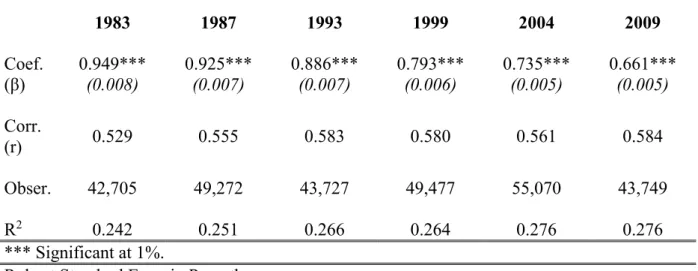
Table 10 and Figure 2 show us the results for the regression coefficient (β) and the correlation (r), per survey year. As years go by, for all birth cohorts, it is clear that we have a considerable decrease in the regression coefficient, from around 0.95, in 1983 to 0.66, in 2009. Meaning, that there was an increase in structural mobility (decrease in persistence). Although, there is a slight expansion in the correlation, it does not vary that much, it goes around 0.57, thus, there is no significant alteration in exchange mobility.
Table 11 and Figure 3 depict the results for transition probabilities (BUM, UCP and UDM), per survey year. We can detect that the growth in mobility observed through the years is mainly caused by a rise in the BUM (upward mobility of children that come from low educated families), which accounted for 0.50, in 1983 and 0.77, in 2009. We are in the presence of a high persistence at the top, around 0.90, and a low downward mobility, around 0.03, that do not have a significant fluctuation through time.
5.1.2. Birth Cohort
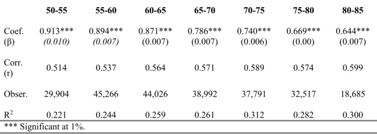
Taking into account the birth cohort effects, Tables 12 and 13 and Figures 4 and 5, illustrate the estimations for β and r and for BUM, UCP and UDM for children’s birth cohorts. Similarly, to the analysis using the years of the surveys, there is evidence of a considerable increasing in structural mobility and a stable exchange mobility, as birth cohorts go by. With the estimated β going from 0.91, for the first birth cohort, to 0.64, for the last, and the estimated r going around 0.56. The BUM is also growing as birth cohorts go by, while the UCP and UDM remain stable at high and low levels, respectively.
The fact that r was stable and β was diminishing is because, as average schooling years become higher, we have initially the standard deviation of children’s years of schooling roughly constant and then after a while decreasing, and at the same time, we have parents’ standard deviation rising and after a while still going up but a lower rate (See Figures 6 and 7). Thus, at first, we have the increasing standard deviation of parents’ education compensating the increase in β and then we have the decrease in standard deviation of children’s education doing it. Moreover, it is observable that, as the standard deviation of children starts declining and the parents’ starts increasing at a lower rate, the ratio between the standard deviations will converge
15
to 1, making β and r converge to each other8. All in all, the choice between these two measures,
will depend on if interpersonal differences in educational attainment are considered relatively to the overall dispersion in attainments or not (Daude, 2011).
Even though, this explains the difference between β and r, it does not give an explanation for the falling trend in persistence.
In general, there is a decreasing persistence driven by an increase in the educational attainment of children that come from low educated parents. And this is something that typically happens when primary school is expanded (Hertz et al., 2007). And, indeed, when looking at the data and connecting it to India’s history and education policy this makes all the sense (which will be further explored in section 5.4.).
5.2. Conditional Regression Results
In this section, the estimates for the beta are presented. Tables 14 and 15 and Figures 8 and 9 show us the results for every survey year and birth cohort, respectively.
In both cases, we can observe that the estimations for the β and the r are lower, representing a higher level of mobility, however the trend that was estimated previously is maintained and the estimates are still robust with the additional controls.9
5.3. Gender Gap Trend
Since, social, cultural and institutional factors may affect men and women’s educational attainment and its mobility differently, this section will provide an overview of the gender disparities and a distinction between mother/father influence on daughter/son in education intergenerational mobility.
Firstly, the several mobility indexes were calculated for two different sets of data: one, only containing observations from female respondents and another, only comprising observations from male respondents. Tables 12 to15 and Figures 10 to 13 portray the results for each survey year, while Tables 16 to 19 and Figures 14 to 17 show the results for each birth cohort. The same trend of the reducing β and steady r is denoted for both daughters and sons, based on a great rise in bottom upward mobility.
8 See Azam & Bhatt, 2012; Daude 2011; Hertz et al., 2007. 9 See Appendix D for the conditional estimations.
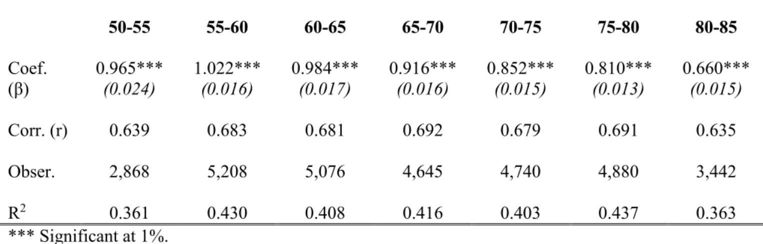
16
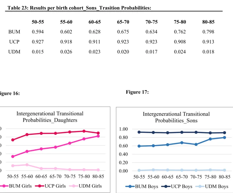
Taking a closer look to Tables 16 and 17, it is detectable that, although, daughters present at the beginning a higher level of persistence compared to sons, this persistence decreases faster to the point where they get similar levels when reaching the last birth cohort. Observing the results for the BUM, UCP and UDM (Tables 18 and 19 and Figures 16 and 17), it is also evident that BUM was more pronounced for daughters than for sons, though when approximating to the youngest cohorts, their BUM’s converge to the same value. Furthermore, when analysing the UDM for daughters we can detect that it is fairly higher for the oldest cohorts, compared with sons. This could be explained by the traditional role of women in the Indian society, which is changing with time. Hence, at the beginning women were not educated even if they came from a family with high socioeconomic status (education is being used as a proxy for socioeconomic status).
Lastly, four different pairs of data sets: mother-daughter; father-daughter; mother-son and father-son were used. Figures 18 to 22 display the results for every index using these groups of data sets, for each survey year and Figures 23 to 27 present the same results for each birth cohort. Mother-daughter and father-daughter data pairs denote a greater level of persistence opposing to mother-son and father-son pairs, though they convert to the same value. Indicating, again, that girls are more dependent on parent education than boys, at first, but then they converge to boys’ values. There are opposite results concerning the mother and father relation to their daughters and sons’ education. When looking at the β, it is observable that the mother-son and mother-daughter pairs demonstrate more persistence compared to the r. Considering the r, it is the father-son and father-daughter pairs that offer higher persistence. This is because fathers present a higher standard deviation in schooling years than mother which will make the ratio between parent and children standard deviations higher for the father pairs, getting, as a consequence, a higher r.
Bottom upward mobility has the same increasing trend with the data pairs for daughters lower, but converging to sons. UCP remains high and stable for all data pairs. Even though, it is clear that the UDM for the father-daughter data pair offers a higher value in earlier cohorts, decreasing as years go by and reaching in the end a similar value as the other data pairs present. Bearing in mind that the UDM represents the probability of children having low educational attainment knowing that their parents have a high level of education, this confirms what was said previously, daughters of educated fathers did not get education due to their traditional role of women in society.
17
5.4. Macroeconomic and Institutional Association Factors
This section will analyse the association of the results obtained with macroeconomic indicators and education policy in India.
Firstly, a descriptive analysis, focused on the relation of the regression coefficient with indicators of economic performance in India, will be performed. Figures 28 to 31 depict scatter plots and linear fits of the regression coefficient with these indicators. Lastly, an overview of post-independence (and until the studied period) Indian’s education policy will be provided in order to be able to associate it with our results.
5.4.1. Macroeconomic Association Factors
Starting with the descriptive analysis, we have that lower values for β (higher intergenerational mobility values) are related with higher values for GDP per capita and salary income (See Figures 28 and 29). Also, there is evidence of a positive correlation between the beta and poverty, measured by poverty headcount (See Figure 30). Thus, it is verified that intergenerational mobility is accompanied by higher levels of wealth.10 In addition, the Gini
Index (as a measure of inequality) (See Figure 31) has been plotted against our regression coefficient, and here, it is observed a slight change in this index through the years. It is still detectable that for the last years the decrease in β is being connected with a small decrease in the Gini Index. This could be explained by the fact that the effect education has on income takes time to occur. Hence, more time is required in order to detect the effects of increasing mobility in income inequality, during the analysed period.
5.4.2. Institutional Association Factors
When India became independent in 1947, there was a great level of illiteracy, the first national census in 1951 accounted for only 9% of women and 27% of men being literate. Therefore, when the constitution was composed, it was decided that the new Indian state would provide free and compulsory education to all children until the age of 14 until 1960, and, even though, this was not at all fulfilled, it continued to be a policy goal for the next 50 years, showing improvement through a lot of educational outcome indicators (Kingdon, 2007).
During the 50’s, there was a distinct policy which aimed for an inclusive education system. Which started by securing free and compulsory primary education to every child, using the
18
Constitution for the new independent Indian State (as mentioned above). The Government’s main objective was to fill in the gap between rural and urban, male and female, and rich and poor. Following this, throughout the 60’s, policy was directed to attend the need to accelerate the expansion and development of the education system, as first goals to be achieved by 1960 had not been yet succeeded. Especially through the National Education Policy implemented in 1968. This policy framework’s biggest accomplishment was the acceptance of a common structure of education throughout the country and the introduction of the 10+2+3 system by most of the States. Furthermore, the school network was highly increased, getting a growth of nearly 65% in the total number of schools until 1981. When reaching the mid 80’s, the Indian Government set some alterations to the National Education Policy of 1968 due to the fact that previous policy was not facing the necessity of removal of the disparities and equalization of educational opportunities to women, scheduled castes and tribes, handicapped people and minority groups. Hence, in 1986 the New Education Policy was implemented. Finally, in the course of the 90’s, universalization of elementary education, elevation of poverty, population control, promotion of women’s equality and education of women were established as goals. Thus, in 1992, so as to achieve these, there was another alteration to the New Education Policy of 1986 (Ghosh, 2007).11
The findings obtained in section 5.2. showed that there was a clear increase in mobility through the years which had as a key driver an increase in the level of education of children with low educated parents. This goes in line with what was just exposed about India’s education policy. Looking closely to the estimates, we can detect a steeper decrease in the regression coefficient and a sharper increase in the BUM (more educated children from less educated parents) for people born in the 60’s.
Considering the results in section 5.3., we have that the diminishing gender gap in mobility (mobility growing faster for females compared with males) throughout the years is being accompanied by a changing policy that focuses more and more in reducing gender disparities in education, by getting women more educated. Moreover, by taking a closer look to the regression coefficient estimates for daughters and sons in comparison, it is detectable a steeper decrease in the beta for daughters born in between 1975-1985.
All in all, it can be said that intergenerational mobility in India is associated with India’s positive economic performance and with its expansive education policy. Even though, the main
19
goal of this paper is not getting into causal relationships for intergenerational mobility, it is something that could be scope in future research on the topic.
6. Conclusion
As expected, considering the general increase in education in India for the studied period, it is shown that intergenerational mobility in education has been increasing considerably through the years. Moreover, it seems that this decrease in persistence has been caused by an increase in the mobility of children that come from low educated families. After controlling for other factors and getting smaller values for these estimates, the trend of significant increase in mobility through the years is maintained. Furthermore, it is observed an extremely high persistence at the top, meaning children of high educated parents tend to be highly educated themselves. Taking into account gender heterogeneity, a closing gender gap in mobility throughout the years was demonstrated. Also, that even though, there is a difference in the relationship between fathers and mothers in their children’s education, they both follow the growing intergenerational mobility trend. Additionally, it was verified an association of positive economic performance and expansive education policy with increasing mobility. It should be highlighted that, the main objective of this paper was not to obtain causal relationships. These results are useful to underline and understand some potential mechanisms. Hence, these could be a starting point for future research.
This paper provided a complete estimation and analysis of intergenerational mobility in education for India in line with the existing literature. Although, there was a limitation to this study. The fact that the surveys used did not comprise retrospective questions on parents’ education, meaning we only had access to information on parents’ education through co-residency of children and their parents. As a result, there was a loss of observations from the surveys, making our sample more represented by younger individuals, since these individuals are the ones that are more likely to live with their parents.
All things considered, this paper gave a new take on intergenerational mobility for India, offering an overview on what drove the estimated mobility (in terms of direction), on the different influences of mother and father in males and females’ educational attainment and on the association factors of the Indian economy and education policy.
20
7. References:
Azam, M., Bhatt, V. (2012). Like Father Like Son? Intergenerational Education Mobility in
India. (IZA Discussion Paper No. 6549).
Becker, G.S., Tomes, N. (1979). An Equilibrium Theory of the Distribution and Income and Intergenerational Mobility. The Journal of Political Economy, 87(6), 1153-1189.
Black, S. E. & Devereux P. (2011). Recent Developments in Intergenerational Mobility. (NBER Working Paper No. 15889).
Chevalier, A., Denny, K., McMahon, D. (2003). A multi-country study of inter-generational
educational mobility. (Paper presented at RC28 meeting, University of Tokyo, March).
Corak, M. (2013). Income Inequality, Equality of Opportunity, and Intergenerational Mobility. (IZA Discussion Paper No. 7520).
Daude, C. (2011). Ascendance by descendants? On intergenerational education mobility in
Latin America. (OECD Development Centre Working Paper No. 297).
Ghosh, S. C. (2007). School Education System in India before and after Independence. In Rawat Publications (Ed.), History of Education in India (pp.113-118). Retrieved from: http://shodhganga.inflibnet.ac.in/bitstream/10603/69112/5/chapter%203.pdf
Hertz, T., Jayasundera, T., Piraino, P.,Selcuk, S., Smith, N., Verashchagina, A. (2007). The Inheritance of Educational Inequality: International Comparisons and Fifty-Year Trends. The
B.E. Journal of Economic Analysis & Policy, 7(12), art. 10.
Hnatkovskay V., Lahiriy A., Paul S. B. (2012). Breaking the Caste Barrier: Intergenerational Mobility in India. The Journal of Human Resources, 48(2), 435-473.
Jänti, M., Jenkins P.S. (2013). Income Mobility. (IZA Discussion Paper No. 7730).
Jalan, J., Murgai, R. (2008). Intergenerational Mobility in Education in India. (Paper Presented at the Indian Statistical Institute, Delhi).
Kingdon, G.G. (2007). The Progress of School Education in India. Oxford Review of Economic
Policy, 23 (2), 168–195.
Markandya, A. (1982). Intergenerational Exchange Mobility and Economic Welfare. European
21
Minnesota Population Center, Integrated Public Use Microdata Series, International: Version 6.5 [dataset]. (2017). Socio-Economic Survey, Household Schedule 10: Employment and Unemployment years 1983, 1987, 1993, 1999, 2004 and 2009 [Data files and codebook]. Minneapolis, MN: University of Minnesota.
Neidhöfer, G., Serrano, J., Gasparini, L. (2017). Educational Inequality and Intergenerational
Mobility in Latin America: A New Database. (School of Business & Economics: Economics
Discussion Paper No. 2017/20).
Organization For Economic Co-operation and Development (OECD) (2014). India Policy
Brief. Retrieved from:
https://www.oecd.org/investment/Encouraging-Greater-International-Investment-in-India.pdf.
Solon, G. (1992). Intergenerational Income Mobility in the United States. The American
Economic Review, 82(3), 393-408.
Solon, G. (2004). A model of intergenerational mobility variation over time and place. In M. Corak (Ed.), Generational income mobility in North America and Europe (pp. 38-47). Cambridge, US: Cambridge University Press.
Zimmerman, D. J. (1992). Regression Toward Mediocrity in Economics Stature. The
22
8. Tables and Figures:
Source: Corak (2013)
23
Table 1: Sample:
Number of Observations per birth cohort Survey Year: 1983 1987 1993 1999 2004 2009 Total Birth Cohort 1920-1925 0.69 % 296 --- --- --- --- --- 296 1925-1930 1.46% 625 0.77% 380 --- --- --- --- 1,005 1930-1935 3.62% 1,545 1.89% 929 0.74% 322 --- --- --- 2,796 1935-1940 5.42% 2,316 3.44% 1,695 1.54% 675 0.46% 229 --- --- 4,915 1940-1945 9.67% 4,128 6.17% 3,041 3.56% 1,558 1.54% 762 0.36% 197 --- 9,686 1945-1950 13.78% 5,886 9.23% 4,547 5.28% 2,310 3.09% 1,530 1.50% 828 0.48% 210 15,311 1950-1955 26.72% 11,410 17.88% 8,812 9.98% 4,364 5.89% 2,919 2.88% 1,588 1.87% 816 29,909 1955-1960 38.63% 16,499 26.83% 13,218 14.41% 6,302 9.28% 4,598 5.83% 3,212 3.30% 1,445 45,274 1960-1965 --- 33.79% 16,650 27.02% 11,815 15.61% 7,735 9.13% 5,028 6.43% 2,814 44,042 1965-1970 --- --- 37.46% 16,381 19.73% 9,781 15.76% 8,680 9.53% 4,170 39,012 1970-1975 --- --- --- 37.86% 18,767 21.99% 12,108 15.87% 6,945 37,820 1975-1980 --- --- --- 6.54% 3,243 36.06% 19,856 21.54% 9,425 32,524 1980-1985 --- --- --- --- 6.49% 3,573 34.54% 15,112 18,685 1985-1990 --- --- --- --- --- 6.43% 2,812 2,812
24
Table 2: Educational Attainment* Number of Years:
No schooling 0
Some primary completed 1
Primary (5 years) completed 5
Lower secondary general completed 8 Secondary, general track completed 10 Post-Secondary technical education 12
Some college completed 13
University completed 15
25
Table 3: Average Years of Schooling_ Parents Survey Year:
1983 1987 1993 1999 2004 2009
Birth Cohort Mean Dev. Mean Std. Dev. Mean Std. Dev. Mean Std. Dev. Mean Std. Dev. Mean Std. Dev. Std.
1920-1925 0.48 1.95 --- --- --- --- --- --- --- --- --- --- 1925-1930 0.75 2.24 0.75 2.16 --- --- --- --- --- --- --- --- 1930-1935 0.61 1.90 0.84 2.50 1.08 2.66 --- --- --- --- --- --- 1935-1940 0.76 2.17 0.84 2.23 1.12 2.87 0.97 2.30 --- --- --- --- 1940-1945 0.89 2.29 1.03 2.50 1.20 2.87 1.13 2.76 0.70 2.07 --- --- 1945-1950 1.07 2.42 1.21 2.63 1.37 2.96 1.40 3.00 1.18 2.75 1.13 2.69 1950-1955 1.41 2.72 1.56 2.90 1.50 3.01 1.63 3.21 1.29 2.77 1.39 3.02 1955-1960 1.75 2.90 1.81 3.06 1.76 3.13 1.82 3.30 1.53 3.02 1.69 3.23 1960-1965 --- --- 2.04 3.16 2.30 3.50 2.13 3.52 1.84 3.28 2.08 3.57 1965-1970 --- --- --- --- 2.76 3.74 2.79 3.93 2.30 3.58 2.45 3.81 1970-1975 --- --- --- --- --- --- 3.12 4.01 2.98 3.95 3.16 4.17 1975-1980 --- --- --- --- --- --- 3.57 4.11 3.32 4.00 3.81 4.31 1980-1985 --- --- --- --- --- --- --- --- 3.64 4.10 4.08 4.30 1985-1990 --- --- --- --- --- --- --- --- --- --- 4.30 4.21
26
Table 4: Average Years of Schooling_ Children Survey Year:
1983 1987 1993 1999 2004 2009
Birth Cohort Mean Dev. Mean Std. Dev. Mean Std. Dev. Mean Std. Dev. Mean Std. Dev. Mean Std. Dev. Std.
1920-1925 2.87 4.25 --- --- --- --- --- --- --- --- --- --- 1925-1930 3.83 4.41 3.93 4.77 --- --- --- --- --- --- --- --- 1930-1935 3.57 4.48 4.47 4.80 5.28 5.24 --- --- --- --- --- --- 1935-1940 4.06 4.65 4.62 4.90 5.62 5.34 5.37 5.38 --- --- --- --- 1940-1945 4.17 4.67 5.18 4.98 6.00 5.36 6.52 5.53 5.86 5.49 --- --- 1945-1950 4.80 4.80 5.55 5.06 6.65 5.42 6.95 5.43 6.88 5.40 7.00 5.55 1950-1955 5.21 4.86 5.92 4.99 6.63 5.33 7.04 5.45 6.97 5.34 7.81 5.36 1955-1960 5.40 4.76 5.94 4.96 6.69 5.30 7.03 5.35 7.00 5.22 7.96 5.21 1960-1965 --- --- 5.86 4.90 7.03 5.31 7.18 5.33 7.30 5.21 8.09 5.15 1965-1970 --- --- --- --- 7.29 5.16 7.79 5.23 7.55 5.17 8.46 5.09 1970-1975 --- --- --- --- --- --- 7.85 5.10 8.21 5.03 8.99 4.83 1975-1980 --- --- --- --- --- --- 8.21 4.81 8.23 4.81 9.42 4.64 1980-1985 --- --- --- --- --- --- --- --- 8.40 4.65 9.32 4.55 1985-1990 --- --- --- --- --- --- --- --- --- --- 9.39 4.34
27
Table 5: Number of Observations Survey Year: 1983 1987 1993 1999 2004 2009 Parents: Mothers 37,764 88% 43,731 89% 39,181 90% 44,833 90% 50,155 91% 40,051 92% Fathers 26,630 62% 32,600 66% 29,051 66% 34,001 69% 37,855 69% 30,567 70% Children: Daughters 4,987 12% 5,456 11% 4,845 11% 6,046 12% 7,259 13% 5,826 13% Sons 37,718 88% 43,816 89% 38,879 89% 43,518 88% 47,811 87% 37,923 87%
28
Table 6: Average Years of Schooling:
Mothers: Fathers: Survey Year: Survey Year:
1983 1987 1993 1999 2004 2009 1983 1987 1993 1999 2004 2009 Birth Cohort 1920-1925 0.24 --- --- --- --- --- 1.92 --- --- --- --- --- 1925-1930 0.34 0.47 --- --- --- --- 2.64 2.05 --- --- --- --- 1930-1935 0.40 0.46 0.65 --- --- --- 1.72 2.53 3.12 --- --- --- 1935-1940 0.46 0.51 0.79 0.63 --- --- 1.90 2.29 2.60 2.37 --- --- 1940-1945 0.49 0.61 0.74 0.75 0.38 --- 2.15 2.46 2.78 2.61 2.33 --- 1945-1950 0.65 0.77 0.86 0.98 0.89 0.88 2.17 2.53 3.09 3.13 2.60 2.38 1950-1955 0.86 0.96 0.95 0.98 0.89 1.03 2.53 2.85 3.07 3.51 2.83 3.05 1955-1960 1.07 1.12 1.13 1.17 1.00 1.30 2.81 3.02 3.24 3.55 3.31 3.18 1960-1965 --- 1.28 1.53 1.39 1.25 1.46 --- 3.16 3.76 3.84 3.55 3.99 1965-1970 --- --- 1.91 1.91 1.59 1.70 --- --- 4.07 4.46 4.02 4.42 1970-1975 --- --- --- 2.20 2.07 2.30 --- --- --- 4.56 4.63 5.17 1975-1980 --- --- --- 2.56 2.30 2.74 --- --- --- 4.94 4.83 5.70 1980-1985 --- --- --- --- 2.67 3.02 --- --- --- --- 4.97 5.69 1985-1990 --- --- --- --- --- 3.19 --- --- --- --- --- 5.86
29
Table 7: Standard Deviation Years of Schooling:
Mothers: Fathers: Survey Year: Survey Year:
1983 1987 1993 1999 2004 2009 1983 1987 1993 1999 2004 2009 Birth Cohort 1920-1925 1.43 --- --- --- --- --- 3.81 --- --- --- --- --- 1925-1930 1.31 1.64 --- --- --- --- 4.30 3.56 --- --- --- --- 1930-1935 1.52 1.76 1.89 --- --- --- 3.32 4.31 4.47 --- --- --- 1935-1940 1.71 1.70 2.31 1.68 --- --- 3.42 3.88 4.43 3.78 --- --- 1940-1945 1.70 1.93 2.26 2.23 1.50 --- 3.71 3.96 4.31 4.20 3.76 --- 1945-1950 1.98 2.17 2.36 2.50 2.43 2.40 3.61 3.96 4.41 4.48 3.95 3.60 1950-1955 2.29 2.44 2.44 2.49 2.31 2.62 3.83 4.05 4.37 4.71 4.09 4.24 1955-1960 2.53 2.63 2.64 2.73 2.48 2.95 3.93 4.15 4.39 4.66 4.39 4.42 1960-1965 --- 2.83 3.11 3.03 2.83 3.09 --- 4.16 4.64 4.79 4.56 4.84 1965-1970 --- --- 3.44 3.53 3.21 3.34 --- --- 4.75 5.07 4.80 5.04 1970-1975 --- --- --- 3.77 3.62 3.85 --- --- --- 5.03 5.02 5.21 1975-1980 --- --- --- 3.97 3.79 4.10 --- --- --- 4.99 4.98 5.24 1980-1985 --- --- --- --- 3.97 4.23 --- --- --- --- 4.95 5.12 1985-1990 --- --- --- --- --- 4.19 --- --- --- --- --- 4.96
30
Table 8: Average Years of Schooling:
Daughters: Sons:
Survey Year: Survey Year:
1983 1987 1993 1999 2004 2009 1983 1987 1993 1999 2004 2009 Birth Cohort 1920-1925 1.67 --- --- --- --- --- 2.92 --- --- --- --- --- 1925-1930 2.05 2.00 --- --- --- --- 3.96 4.02 --- --- --- --- 1930-1935 2.97 2.65 4.97 --- --- --- 3.62 4.58 5.32 --- --- --- 1935-1940 2.27 3.41 3.88 2.38 --- --- 4.21 4.69 5.76 5.45 --- --- 1940-1945 2.35 3.39 3.94 3.93 5.13 --- 4.37 5.32 6.16 6.69 5.89 --- 1945-1950 2.90 3.38 4.12 4.50 4.44 6.00 5.00 5.76 6.88 7.17 7.12 7.14 1950-1955 3.82 4.15 4.58 4.65 4.22 5.18 5.39 6.09 6.82 7.26 7.28 8.06 1955-1960 5.50 5.11 5.21 4.57 4.77 5.80 5.38 6.04 6.83 7.27 7.21 8.16 1960-1965 --- 6.12 5.87 5.44 5.23 5.13 --- 5.82 7.15 7.37 7.53 8.35 1965-1970 --- --- 7.67 6.50 5.54 6.50 --- --- 7.22 7.95 7.77 8.63 1970-1975 --- --- --- 7.79 6.70 7.52 --- --- --- 7.86 8.40 9.14 1975-1980 --- --- --- 8.95 8.39 8.77 --- --- --- 8.03 8.20 9.50 1980-1985 --- --- --- --- 9.13 10.04 --- --- --- --- 8.17 9.17 1985-1990 --- --- --- --- --- 10.34 --- --- --- --- --- 9.05
31
Table 9: Standard Deviation Years of Schooling:
Daughters: Sons:
Survey Year: Survey Year:
1983 1987 1993 1999 2004 2009 1983 1987 1993 1999 2004 2009 Birth Cohort 1920-1925 4.44 --- --- --- --- --- 4.25 --- --- --- --- --- 1925-1930 4.03 4.23 --- --- --- --- 4.41 4.78 --- --- --- --- 1930-1935 4.09 3.95 5.03 --- --- --- 4.51 4.83 5.27 --- --- --- 1935-1940 3.99 5.08 4.63 3.46 --- --- 4.68 4.88 5.37 5.41 --- --- 1940-1945 3.81 4.75 5.22 5.17 5.89 --- 4.71 4.97 5.34 5.51 5.48 --- 1945-1950 4.10 4.57 5.00 5.06 5.02 6.04 4.82 5.06 5.40 5.41 5.38 5.49 1950-1955 4.81 4.88 5.09 5.21 4.68 5.35 4.84 4.96 5.31 5.42 5.32 5.30 1955-1960 5.25 5.23 5.37 5.05 5.19 5.67 4.67 4.93 5.27 5.32 5.18 5.12 1960-1965 --- 5.45 5.53 5.23 5.18 5.17 --- 4.80 5.27 5.30 5.17 5.06 1965-1970 --- --- 5.53 5.45 5.34 5.43 --- --- 5.09 5.18 5.11 5.02 1970-1975 --- --- --- 5.57 5.44 5.311 --- --- --- 5.02 4.95 4.76 1975-1980 --- --- --- 5.21 5.31 5.16 --- --- --- 4.68 4.71 4.56 1980-1985 --- --- --- --- 4.94 4.84 --- --- --- --- 4.54 4.48 1985-1990 --- --- --- --- --- 4.43 --- --- --- --- --- 4.25
32
Table 10: Results per survey year_Unconditional Regression Coefficient and Correlation 1983 1987 1993 1999 2004 2009 Coef. (β) 0.949*** (0.008) 0.925*** (0.007) 0.886*** (0.007) 0.793*** (0.006) 0.735*** (0.005) 0.661*** (0.005) Corr. (r) 0.529 0.555 0.583 0.580 0.561 0.584 Obser. 42,705 49,272 43,727 49,477 55,070 43,749 R2 0.242 0.251 0.266 0.264 0.276 0.276 *** Significant at 1%.
Robust Standard Error in Parentheses
Table 11: Results per survey year_Trasition Probabilities
1983 1987 1993 1999 2004 2009 BUM 0.502 0.556 0.609 0.649 0.701 0.777 UCP 0.890 0.894 0.908 0.915 0.907 0.876 UDM 0.034 0.032 0.025 0.026 0.025 0.019 0.00 0.20 0.40 0.60 0.80 1.00 1983 1987 1993 1999 2004 2009 Intergenerational Transitional Probabilities
BUM UCP UDM
0.00 0.20 0.40 0.60 0.80 1.00 1983 1987 1993 1999 2004 2009
Regression Coeficient and Correlation
Coef. (β) Corr. (r)
33
Table 12: Results per Birth Cohort_Unconditional Regression Coefficient and Correlation 50-55 55-60 60-65 65-70 70-75 75-80 80-85 Coef. (β) 0.913*** (0.010) 0.894*** (0.007) 0.871*** (0.007) 0.786*** (0.007) 0.740*** (0.006) 0.669*** (0.00) 0.644*** (0.007) Corr. (r) 0.514 0.537 0.564 0.571 0.589 0.574 0.599 Obser. 29,904 45,266 44,026 38,992 37,791 32,517 18,685 R2 0.221 0.244 0.259 0.261 0.312 0.282 0.300 *** Significant at 1%.
Robust Standard Error in Parentheses
Table 13: Results per birth cohort_Trasition Probabilities:
50-55 55-60 60-65 65-70 70-75 75-80 80-85 BUM 0.570 0.582 0.609 0.658 0.699 0.749 0.791 UCP 0.911 0.906 0.902 0.917 0.917 0.910 0.920 UDM 0.025 0.031 0.029 0.025 0.022 0.024 0.018 0.00 0.20 0.40 0.60 0.80 1.00 50-55 55-60 60-65 65-70 70-75 75-80 80-85
Regression Coefficient and Correlation
Coef. (β) Corr. (r) 0.00 0.20 0.40 0.60 0.80 1.00 50-55 55-60 60-65 65-70 70-75 75-80 80-85 Intergenerational Transitional Probabilities
BUM UCP UDM
34 Figure 6: Figure 7: 0.00 1.00 2.00 3.00 4.00 5.00 6.00 50-55 55-60 60-65 65-70 70-75 75-80 80-85
Standard Deviations of Years of Schooling
Parents Children 0.00 2.00 4.00 6.00 8.00 10.00 50-55 55-60 60-65 65-70 70-75 75-80 80-85
Average Years of Schooling
35
Table 14: Results per survey year_Conditional Regression Coefficient and Correlation 1983 1987 1993 1999 2004 2009 Coef. (β) 0.802*** (0.009) 0.803*** (0.008) 0.782*** (0.008) 0.717*** (0.006) 0.669*** (0.006) 0.610*** (0.006) Corr. (r) 0.448 0.482 0.516 0.525 0.511 0.539 Obser. 41,963 48,583 43,241 48,908 54,768 43,544 R2 0.304 0.293 0.298 0.293 0.298 0.290 *** Significant at 1%.
Robust Standard Error in Parentheses
0.00 0.20 0.40 0.60 0.80 1.00 1983 1987 1993 1999 2004 2009
Regression Coefficient and Correlation
Coef. (β) Corr. (r)
36
Table 15: Results per Birth Cohort_Conditional Regression Coefficient and Correlation 50-55 55-60 60-65 65-70 70-75 75-80 80-85 Coef. (β) 0.771*** (0.010) 0.780*** (0.008) 0.772*** (0.007) 0.715*** (0.007) 0.690*** (0.007) 0.623*** (0.006) 0.610*** (0.008) Corr. (r) 0.433 0.469 0.501 0.519 0.550 0.535 0.568 Obser. 29,462 44,692 43,578 38,604 37,501 32,336 18,594 R2 0.297 0.306 0.307 0.293 0.306 0.296 0.308 *** Significant at 1%.
Robust Standard Error in Parentheses
0.00 0.20 0.40 0.60 0.80 1.00 50-55 55-60 60-65 65-70 70-75 75-80 80-85
Regression Coefficient and Correlation
Coef. (β) Corr. (r)
37
Table 16: Results per survey year_Daughter_Regression Coefficient and Correlation
1983 1987 1993 1999 2004 2009 Coef. (β) 1.037*** (0.016) 1.030*** (0.002) 0.996*** (0.016) 0.913*** (0.013) 0.866*** (0.012) 0.779*** (0.012) Corr. (r) 0.690 0.696 0.722 0.705 0.676 0.691 Obser. 4,987 5,456 4,845 6,002 7,259 5,826 R2 0.452 0.443 0.440 0.434 0.428 0.404 *** Significant at 1%.
Robust Standard Error in Parentheses
Table 17: Results per survey year_Sons_Regression Coefficient and Correlation
1983 1987 1993 1999 2004 2009 Coef. (β) 0.957*** (0.009) 0.924*** (0.008) 0.883*** (0.008) 0.786*** (0.007) 0.723*** (0.006) 0.650*** (0.006) Corr. (r) 0.514 0.542 0.571 0.568 0.547 0.570 Obser. 37,715 43,815 38,879 43,475 47,811 37,923 R2 0.228 0.236 0.253 0.251 0.260 0.262 *** Significant at 1%.
Robust Standard Error in Parentheses
0.00 0.20 0.40 0.60 0.80 1.00 1.20 1983 1987 1993 1999 2004 2009
Regression Coeffcient and Correlation_Daughters
Coef. Girls (β) Corr. Girls (r)
0.00 0.20 0.40 0.60 0.80 1.00 1.20 1983 1987 1993 1999 2004 2009
Regression Coefficient and Correlation_Sons
Coef. Boys (β) Corr. Boys (r)
38
Table 18: Results per survey year_Daughters_Trasition Probabilities
1983 1987 1993 1999 2004 2009
BUM 0.336 0.393 0.463 0.516 0.561 0.684
UCP 0.852 0.862 0.875 0.895 0.893 0.918
UDM 0.034 0.049 0.006 0.048 0.036 0.029
Table 19: Results per survey year_Sons_Trasition Probabilities
1983 1987 1993 1999 2004 2009 BUM 0.521 0.574 0.625 0.666 0.719 0.788 UCP 0.902 0.902 0.915 0.920 0.910 0.930 UDM 0.033 0.027 0.020 0.021 0.023 0.016 0.00 0.20 0.40 0.60 0.80 1.00 1983 1987 1993 1999 2004 2009
Intergenerational Transition
Probabilities_Daughters
BUM Girls UCP Girls UDM Girls
0.00 0.20 0.40 0.60 0.80 1.00 1983 1987 1993 1999 2004 2009
Intergenerational Transition
Probabilities_Sons
BUM Boys UCP Boys UDM Boys
39
Table 20:Results per Birth Cohort_Regression Coefficient and Correlation_Daughters:
50-55 55-60 60-65 65-70 70-75 75-80 80-85 Coef. (β) 0.965*** (0.024) 1.022*** (0.016) 0.984*** (0.017) 0.916*** (0.016) 0.852*** (0.015) 0.810*** (0.013) 0.660*** (0.015) Corr. (r) 0.639 0.683 0.681 0.692 0.679 0.691 0.635 Obser. 2,868 5,208 5,076 4,645 4,740 4,880 3,442 R2 0.361 0.430 0.408 0.416 0.403 0.437 0.363 *** Significant at 1%.
Robust Standard Error in Parentheses
Table 21: Results per Birth Cohort_Regression Coefficient and Correlation_Sons:
50-55 55-60 60-65 65-70 70-75 75-80 80-85 Coef. (β) 0.916*** (0.011) 0.891*** (0.008) 0.865*** (0.008) 0.779*** (0.007) 0.731*** (0.007) 0.651*** (0.007) 0.639*** (0.008) Corr. (r) 0.509 0.525 0.555 0.561 0.582 0.557 0.586 Obser. 27,036 40,058 38,950 34,345 33,051 27,637 15,243 R2 0.217 0.237 0.251 0.251 0.275 0.262 0.281 *** Significant at 1%.
Robust Standard Error in Parentheses
0.00 0.20 0.40 0.60 0.80 1.00 50-55 55-60 60-65 65-70 70-75 75-80 80-85
Regression Coefficient and Correlation_ Sons
Coef. Boys (β) Corr. Boys (r)
Figure 15: 0.00 0.20 0.40 0.60 0.80 1.00 50-55 55-60 60-65 65-70 70-75 75-80 80-85
Regression Coefficient and Correlation_Daghters
Coef. Girls (β) Corr. Girls (r)
40
Table 22: Results per birth cohort_Daughters_Trasition Probabilities:
50-55 55-60 60-65 65-70 70-75 75-80 80-85
BUM 0.334 0.455 0.516 0.557 0.652 0.754 0.822
UCP 0.731 0.857 0.886 0.888 0.919 0.939 0.894
UDM 0.114 0.137 0.047 0.047 0.021 0.018 0.015
Table 23: Results per birth cohort_Sons_Trasition Probabilities:
50-55 55-60 60-65 65-70 70-75 75-80 80-85 BUM 0.594 0.602 0.628 0.675 0.634 0.762 0.798 UCP 0.927 0.918 0.911 0.923 0.923 0.908 0.913 UDM 0.015 0.026 0.023 0.020 0.017 0.024 0.018 0.00 0.20 0.40 0.60 0.80 1.00 50-55 55-60 60-65 65-70 70-75 75-80 80-85 Intergenerational Transitional Probabilities_Daughters
BUM Girls UCP Girls UDM Girls
Figure 16: Figure 17: 0.00 0.20 0.40 0.60 0.80 1.00 50-55 55-60 60-65 65-70 70-75 75-80 80-85 Intergenerational Transitional Probabilities_Sons
41 0.00 0.20 0.40 0.60 0.80 1.00 1983 1987 1993 1999 2004 2009
Correlation (r)_Father vs Mother
Corr. Mother-Daughter Corr. Mother-Son
Corr. Father-Daughter Corr. Father-Son
0.00 0.20 0.40 0.60 0.80 1.00 1.20 1983 1987 1993 1999 2004 2009
Regression Coeficient (β)_Father vs Mother
Coef. Mother-Daughter Coef. Mother-Son
Coef. Father-Daughter Coef. Father-Son
Figure 18:
42 0.00 0.20 0.40 0.60 0.80 1.00 1983 1987 1993 1999 2004 2009 BUM_Father vs Mother
BUM Mother-Daughter BUM Father-Daughter
BUM Mother-Son BUM Father-Son
0.00 0.20 0.40 0.60 0.80 1.00 1983 1987 1993 1999 2004 2009 UCP_Father vs Mother
UCP Mother-Daughter UCP Father-Daughter
UCP Mother-Son UCP Father-Son
0 0.03 0.06 0.09 0.12 0.15 1983 1987 1993 1999 2004 2009 UDM_Father vs Mother
UDM Mother-Daughter UDM Father-Daughter
UDM Mother-Son UDM Father-Son
Figure 20:
Figure 21:
43 0.00 0.10 0.20 0.30 0.40 0.50 0.60 0.70 0.80 50-55 55-60 60-65 65-70 70-75 75-80 80-85
Correlation (r)_Father vs Mother
Corr. Mother-Daughter Corr. Mother-Son
Corr. Father-Daughter Corr. Father-Son
0.00 0.20 0.40 0.60 0.80 1.00 1.20 50-55 55-60 60-65 65-70 70-75 75-80 80-85
Regression Coefficient (β)_Father vs Mother
Coef. Mother-Daughter Coef. Mother-Son
Coef. Father-Daughter Coef. Father-Son
Figure 23: