Educational Systems, Intergenerational Mobility and
Social Segmentation
Nathalie Chusseau1, Joël Hellier2
Abstract
We show that the very characteristics of educational systems generate social segmentation. A stylised educational framework is constructed in which everyone receives a compulsory basic education and can subsequently choose between direct working, vocational studies and university. There is a selection for entering the university which consists of a minimum human capital level at the end of basic education. In the model, an individual’s human capital depends (i) on her/his parents’ human capital, (ii) on her/his schooling time, and (iii) on public expenditure for education. There are three education functions corresponding to each type of study (basic, vocational, university). Divergences in total educational expenditure, in its distribution between the three studies and in the selection severity, combined with the initial distribution of human capital across individuals, can result in very different social segmentations and generate under education traps (situations in which certain dynasties remain unskilled from generation to generation) at the steady state. We finally implement a series of simulations that illustrate these findings in the cases of egalitarian and elitist educational systems. Assuming the same initial distribution of human capital between individuals, we find that the first system results in two-segment stratification, quasi income equality and no under education trap whereas the elitist system generates three segments, significant inequality and a large under education trap.
JEL Classification: E24, H52, I21.
Keywords: educational systems; intergenerational mobility; social segmentation; under-education trap
1.
Introduction3In the economic literature, the impact of human capital acquisition upon social segmentation has been analysed through the emergence of under education traps, i.e., situations in which a proportion of the population remains unskilled from generation to generation.
In the early approach of Becker and Tomes (1979) with a perfectly competitive credit market, all the dynasties converge towards the same human capital in the long term. Assuming credit market imperfections, Loury (1981) and Becker and Tomes (1986) show that this convergence still holds but it is slowed down, thereby creating a 'low mobility trap' (Piketty, 2000).
These rather optimistic diagnoses were subsequently questioned by a number of works that analysed the emergence of under education traps. Several determinants can cause the emergence of such traps: a credit constraint with a fixed cost of education (Galor and Zeira, 1993, Barham et al., 1995), an S-shaped education function (Galor and Tsiddon, 1997), a neighbourhood effect resulting from local externalities (Benabou,
1 EQUIPPE, University of Lille 1 and MESHS, France.
2 EQUIPPE, Univ. of Lille 1, MESHS and LEMNA, University of Nantes, France; correspondence address: [email protected]
1993, 1996a, 1996b; Durlauf 1994, 1996), limited parental altruism (Das, 2007) etc. In most of these works, the trap results from non convexities that make certain individuals select low education. However, these approaches typically suppose that the institutional access to education is equally guaranteed. Financial constraints, family and social characteristics and limited abilities are then the main factors that explain the differences in educational choices and the related social segmentation.
However, since Weber (1906), the sociological literature has drawn attention to the fact that the educational system itself can create social segmentation (Bidwell and Friedkin, 1988, for an early review). It has been underlined that the type of knowledge that is promoted corresponds to the cultural backgrounds of the children from the upper and middle classes (Sorokin, 1959; Bourdieu and Passeron, 1970; Baudelot and Establet, 1971) and that families from the lower classes overestimate the cost of and underestimate the return from education (Boudon, 1973, 1974). In addition, because of better information and network effects, the children from higher classes select better educational strategies, and they have access to better positions than children from lower classes even when they possess the same degree (Anderson, 1961; Boudon, 1973, 1974; Thelot, 1982). Finally, a number of analysts have emphasised the influence of the selection pattern, i.e. the very structure of the educational system, on the formation and the persistence of social segmentation (Bourdieu and Passeron, 1970; Bowles and Gintis, 1976). Several recent empirical studies confirm the impact of the educational system upon social stratification. Using data from an international survey, Shavit and Muller (2000) find that the institutional characteristics of the school systems partly explain the differences in educational and occupational attainment across countries. Similarly, by comparing the transition from school to work in France, Germany, the UK and the US, Kerckhoff (2000) concludes that the differences across these countries are partially due to the differences in their educational systems.
If sociologists have studied for a long time the impact of hierarchical educational systems upon social stratification, this has only recently been investigated by the economic theory. Driskill and Horowitz (2002) and Su (2004) analyse hierarchical educational systems by focusing on the allocation of public funding between basic and advanced education. They study the impacts upon growth, welfare and income distribution, but not on social stratification. Bertocchi and Spagat (2004) model a three-level educational system (basic education and secondary education divided between vocational and general studies) so as to analyse social stratification during the different stages of economic development. However, their approach does not generate lasting under education trap because workers without secondary education disappear with the vanishing of the traditional sector.
Our objective is to analyse the impact of the structure of the educational system, i.e., the way the courses of study are organised with their different stages, divisions, selection procedures and funding, upon the formation and the intergenerational persistence of social segmentation.
enforced until the age of 15-18 in advanced countries, and until 12-15 years old in most of the developing countries. After compulsory schooling, young adults can either join the labour market, or pursue their studies. In the latter case, they typically face two courses of study. They can firstly select vocational studies. If such studies do exist in all countries, their shape and entry conditions significantly differ between as well as within countries. Usually, the access to vocational study does not require the obtainment of a final degree that sanctions secondary schooling (A-Level, Abitur, Baccalaureat etc.), even if this is the case for certain technical studies. In addition, vocational studies typically begin at upper secondary school level and can be part of an apprenticeship system. A second course of study consists in going to university, i.e., the tertiary educational system. Entering a university typically requires the obtainment of a degree that sanctions secondary school, and additional selection procedures are often enforced. We firstly construct a simple stylised model that can describe this general educational framework, and that can be declined into various configurations. From this general model, we derive several possible social segmentations depending on the characteristics of the educational system. We finally implement a series of simulations that illustrate different social segmentations resulting from different educational systems.
The article is original in several respects. It firstly develops an intergenerational theoretical framework that allows modelling the impact of the structure of the educational system upon social segmentation. Secondly, the model generates social segmentations that depend on both the educational system and the initial distribution of human capital between households. Finally, different educational systems result in different segmentations for the same initial distribution of human capital.
The main features of the educational general framework are presented in section 2. The educational choices of individuals are analysed in section 3. The characteristics of the educational systems and the related social segmentations are determined in section 4. Section 5 analyses the human capital dynamics and the resulting segmentation. A series of simulations are implemented in section 6. We conclude in section 7.
2.
The model general framework2.1. Production
The economy produces one good with technology Y =ωH, j j
j
H =
∑
t h , hjbeing the human capital of individual j and tj her/his time spent in the production activity. By assuming perfect competition on the market for goods, the profit is nil at equilibrium and ω is the before tax wage per unit of human capital×time. As a consequence, individual j earns the pre-tax income ωj =ωh tj j.
2.2. Individuals and Education
An individual’s life comprises two periods. Being young, s/he receives a basic education. Being adult, s/he lives one period of length 1 that s/he can divide between higher education and work.
The government provides individuals with both basic and higher education. Public education is funded by a tax on the parents' income at rate τ . The after tax wage per unit of human capital×time is thus w= −(1 τ ω) .
Basic education is compulsory and this provides individuals with the human capital necessary to get access to the labour market. In contrast, pursuing higher education is a choice of the individual who takes her/his decision by comparing the related income benefit and cost. Albeit spending the same time in basic education, individuals differ in their human capital at the end of this time. This is because intra-family externalities make children from more educated families more able to acquire the provided education. In addition, it is assumed that the market for credit is perfect and that the interest rate is nil4. These assumptions are tailored so as to place individuals in
the most favourable situation in their choice for higher education, and thereby to focus on the sole impacts (i) of the uneven distribution of human capital across parents and (ii) of the educational structure, on the emergence of social stratifications.
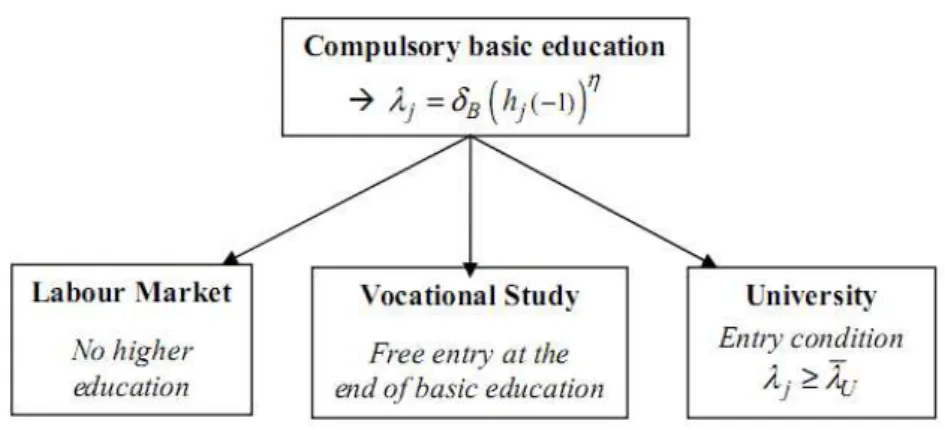
At the end of basic education, an individual can choose, either to join directly the labour market, or to pursue further education. In the latter case, two courses of study are open that are exclusive of each other. The individual can firstly choose vocational studies (denoted V) without any constraint in terms of human capital attainment at the end of basic education. S/He can also go to university (denoted U) if her/his human capital at the end of basic education is at least λU.
2.3. Education functions
Basic education produces individual j's human capital according to the following function:
(
( 1))
j B hj η
λ =δ − (1)
B
δ denotes the productivity in basic education that depends on the government's
educational policy. Expression
(
hj( 1)−)
ηdepicts the intra-family externality, i.e., the impact of the parent’s human capital hj( 1)− on her/his child’s human capital at the end of basic education. We suppose that the marginal impact of the intra-family externality is decreasing, i.e. 0< <η 1.The education function in higher education i, i=V U, is
{
}
max i ,
j i ji j j
h = δe ε λ λ , with δi being the productivity and eji individual j's schooling
time in higher education i, and 0<εi<1. When effective, i.e. for i
i jie j j ε
δ λ >λ , higher education of type i thus depends:
1) on the productivity δi in higher education i, that is produced by the educational policy,
2) on the time eji spent for studying in i with decreasing returns because 0<εi<1, and
3) on the already acquired basic education λj.
Pursuing higher education induces a fixed cost f paid by the individual and assumed to be identical for both types of higher education for the sake of simplicity. This cost consists in a fixed amount of goods, so that f = × =ω k w(1−τ)−1k , with k being the fixed amount of human capital utilised in terms of the fixed cost of education. There is a minimum schooling time for higher education to be effective
( i
i jie ε j j
δ λ >λ ): 1/ i ji i
e >δ − ε . This condition is always fulfilled at the individual’s optimum because further education is only chosen if the related lifetime income is
higher than that from direct working (1 ) i
ji i ji j j
w −e δe ε λ − >f wλ , which implies 1/ i
ji i
e >δ − ε . The education function in study i=V U, can thus be written:
(
)
1/( 1)
i i
B i ji j ji i
j j
e h e
h
η
ε ε
δ δ δ
λ
−
−
⎧ >
⎪ = ⎨ ⎪⎩
iif
otherwise
(2)
A low εi signifies that the marginal gain from education decreases fast, and thus that the knowledge available from the study of type i can be captured rapidly. In return, with a high εi it is necessary to spend more time to acquire the human capital provided by study i. We suppose that εV <εU, i.e., that more time is necessary to acquire the knowledge provided by the university than that provided by vocational studies.
Figure 1. The individual's choices at the end of basic education
As individual j' s human capital at the end of basic education is totally determined
by relation λj =δB
(
hj( 1)−)
η, it is possible to rewrite the entry condition in university in terms of her/his parent's human capital. As a consequence, only individuals whose parent's human capital is higher than hU =(
λ δU / B)
1/η can enter the university.3. Educational choices
Let us consider individual j endowed with human capital λj at the end of basic education. S/He chooses the educational pattern that maximises her/his lifetime income. If s/he chooses not to proceed with further education her/his lifetime income
is wλj, and s/he earns (1 ) i
ji i ji j
w −e δe ε λ − f if s/he selects education i, i = V,U.
To determine the individual's educational choice, we firstly suppose that s/he pursues higher education and we calculate her/his related optimal schooling time. Afterwards, we compare the three possible choices (no further education, vocational study and university), and we select the strategy that maximises the individual's lifetime earning.
3.1. Schooling time
Lemma 1: An individual who selects higher education i, i = V,U, allows time eˆi to this education, with:
ˆi i/ (1 i)
e =ε +ε (3)
Proof: By maximising (1 ) i ji i ji j
Since εV <εU, the time allowed for vocational study eˆV =εV / (1+εV) is lower than that allocated to university eˆU =εU / (1+εU).
3.2. Educational choices
Henceforth, we adopt the following notations:
/(1 )
ˆ ˆ
(1 ) V 1
V V V
k
e e ε τ λ
δ
− ≡
− − (4)
/(1 )
'
ˆ ˆ
(1 ) U 1
U U U
k
e e ε τ λ
δ
− ≡
− − (5)
We denote h and h' the parents’ human capital corresponding to the basic education levels λ and λ', i.e., h =
(
λ δ/ B)
1/η and h'=(
λ δ'/ B)
1/η.Lemma 2: Individual j earns more (less) by working directly than by making vocational studies if λ λj< (λ λj> ) and s/he earns more (less) by working directly than by entering the university if λ λj< ' (λ λj> ').
Proof: Individual j earns more by working directly than by selecting study i, i = V,U, if the former provides her/him with a lifetime income higher than that given by study i, i.e. (1 ˆ ˆ) i
i i i j j
wδ −e eελ − <f wλ . The conditions on λj are obtained by inserting 1
(1 )
f =w −τ − k into this inequality.
The related conditions on individual j’s parent human capital hj( 1)− are (i) ( 1)
j
h − <h for higher earnings from direct working than from vocational studies, and (ii) hj( 1)− <h' for higher earnings from direct working than from entering the university.
Lemma 3: All individuals prefer the university to vocational studies if λ λ> ' (equivalently h >h'), they all prefer vocational studies to the university if λ λ< ' (h <h'), and both choices are equivalent for everyone if λ λ= ' ( h =h').
Proof: Individuals prefer university to vocational studies if the former provides a
higher lifetime income than the latter: (1 ˆ ) ˆ U (1 ˆ ) ˆ V
U U U j V V V j
w −e δ e ε λ >w −e δ e ε λ , i.e.
ˆ ˆ ˆ ˆ
(1 ) U (1 ) V ' '
U eU eUε V e eV Vε h h
studies to university if λ λ< ''⇔ <h h', and both choices provide the same lifetime income if λ λ= '⇔ =h h'.
Proposition 1: Consider individual j with human capital λj at the end of basic education. Then:
1) Individual j joins directly the labour market (i) when λ λj< and λ λj< ' , or (ii) when λ λ λ'≤ <j and λj <λU.
2) Individual j selects vocational studies (i) when λ λ λ≤ <j ', or (ii) when '
j
λ λ λ≥ > and λj <λU.
3) Individual j enters the university when λ λj≥ ', λ λ> ' and λj ≥λU.
Case (1) corresponds to the two situations in which the individual directly joins the labour market. In the first, doing this provides her/him with higher income than selecting, either vocational studies or the university (because λ λj< and λ λj< ', see Lemma 2). In the second, the individual’s income is higher when working directly than when pursuing vocational studies and lower when working directly than when studying in the university (λ λj< and λ λj≥ ', see Lemma 2), but this last option is impossible because her/his human capital at the end of basic education is lower than λU.
Case (2) depicts the two situations in which the individual selects vocational studies. In the first, vocational studies provide her/him with a higher income than both direct working and university (λ λj≥ and λj <λ', Lemma 2). In the second, vocational studies is preferred to direct working (λ λj≥ , Lemma 2), but less profitable than university (λ λ> ', Lemma 3), with this last choice being unachievable because of a lack of human capital at the end of basic education (λj <λU).
By replacing the λs by the related parent’s human capital h( 1)− =
(
λ δ/ B)
1/η, we obtain the corollary proposition:Corollary: Consider individual j whose parent’s human capital is hj( 1)− . Then:
1) Individual j joins directly the labour market (i) when hj( 1)− <h and
( 1) ' j
h − <h , or (ii) when h'≤hj( 1)− <h and hj( 1)− <hU.
2) Individual j selects vocational studies (i) when h h≤ j( 1)− <h', or (ii) when hj( 1)− ≥ >h h' and hj( 1)− <hU.
3) Individual j enters the university when hj( 1)− ≥h', h >h' and
( 1)
j U
h − ≥h .
Finally, the following feature can be established when both V and V are concurrently chosen inside a generation.
Lemma 4: Within the same generation, the coexistence of individuals who prefer V to V and individuals who prefer V to V is impossible. Consequently, if both V and V are selected within the same generation, then, either all the individuals who select V are constrained by the entry threshold λU, or all individuals have the same lifetime earning when choosing V and U.
Proof: see Appendix 1.
4. Educational systems and segmentation
4.1. Educational Systems
The education functions (1) and (2) and the individuals' educational choices depend on the values δi, i=B V U, , . The educational policy determines these values according to the functions:
1
B B
B B B
B
q y e
e β
ε τ
δ =δ ⎛⎜ − ⎞⎟
1 ˆ i
i i
i i
q y e
β
τ δ δ
µ −
⎛ ⎞
= ⎜ ⎟
⎝ ⎠ , i=V U, (7)
i
q is the proportion of total levies allocated to education i (qB+qV +qU =1),
1
y− the total income per capita in the parents' generation, µi the proportion of the current generation involved in study i (since all the individuals follow basic education,
1 B
µ = ) , eB the compulsory schooling time, and coefficients δi indicate the efficiency of public spending in the i-study. It can be noted that, unlike δV and δU, δB integrates the compulsory schooling time in basic education because this is part of the educational policy and because it was not accounted for in the basic education function (1). We also assume 0< <β 1, which indicates that the marginal impact of public spending on education is decreasing.
To provide an interpretation of function (7), let us rewrite it
(
1/ ˆ)
i i q Yi iMei β
δ =δ τ − µ , where Y−1 is the total income of the parents' generation and
M the number of dynasties. The productivity in the i-study depends (i) positively on the amount of levies q Yiτ −1 allocated to i, and (ii) negatively on the number µiM of students involved in i and on the length eˆi of this course of study. Expression
(
q Yiτ −1/µiMeˆi)
is thus the public expense for education i per pupil×schooling time.Definition 1: We call 'Educational System
(
τ,qB,qV,qU,λU,eB)
' the educational pattern that allocates levies τY−1>0 to the three types of studies (B,V,U) in the proportions qB >0, qV ≥0, and qU ≥0, with the entry conditions λU in the university and the compulsory schooling time in basic education eB >0, the public education productivity functions (6) and (7) being given.Features τY−1>0, qB >0 and eB >0 are necessary for the existence of the educational system. In addition, a necessary condition for an educational system to be efficient is µi = ⇒0 qi =0 for i = V,U. This condition signifies that there is no waste of public spending: if nobody chooses study i, thenthe social planner does not allocate funds to this study. Henceforth, we suppose that the social planner never allocates funds to a study which is chosen by no-one.
We denote B
(
)
T B B B
A ≡δ e ε −β q τ β, ˆ V
(
)
V T V V V
A ≡ A δ e ε −β q τ β, and
(
)
ˆ U
U T U U U
schooling. Consequently, the education functions are (by inserting (6) and (7) into (1) and (2)):
(
)
, 1 ( 1)
j T T j
h =A y− β h − η (8)
(
)
2(
)
, ( ) 1 ( 1)
j i i i j
h =A µ t −β y− β h − η, i = V,U (9)
Lemma 5: Everyone prefers the university to vocational studies if and only if 1/
ˆ
(1 )
ˆ
(1 )
V V V
U U U
e A e A
β
µ ρ µ
⎛ − ⎞
> = ⎜ − ⎟
⎝ ⎠ ; everyone prefers vocational studies to university if
and only if V U
µ ρ
µ < ; both studies bring the same lifetime income if and only if
V U
µ ρ
µ = .
Proof: see Appendix 2.
4.2. Segmentation and under-education trap
Segmentation occurs when the individuals inside a generation are divided between several segments (groups) in terms of educational choice and there is an under education trap if certain individuals do not pursue higher education. In the model developed here, there are three possible segments, T (under education trap), V (individuals selecting vocational studies) and V (individuals entering the university). The segmentation can be transitory or lasting. In the first case, certain segments tend to disappear with time.
Definition 2: There is a permanent segmentation if the proportionsµi, i=T V U, , , are constant over time.
There is thus a permanent under education trap if there is a permanent social segmentation such that µT >0. In a situation of permanent under education trap, a constant number of dynasties remain at the basic education level from generation to generation. In the case of steady state segmentation, all these dynasties possess the same constant human capital.
4.3. Segmentation characteristics
A segmentation pattern is characterised by three different dimensions: 1) The number of segments;
2) The weight of each segment as a percentage of the working population; 3) The gaps between the segments in terms of human capital and income.
Acting on these three dimensions through the determinants of the educational system participates in a policy that concerns social inequality. We do not directly address this issue, which would require the choice of a social welfare function, and thus a level of inequality aversion and a time preference (since we have a succession of generations). We just analyse the impact of the educational system determinants
(
τ,qB,qV,qU,λU,eB)
and of the real product per capita on the aforementioned characteristics.Firstly, the number of individuals inside the under education trap tends (i) to decrease with a rise in shares qB and qV of the levies allowed for basic education and vocational studies, (ii) to decrease with the income per capita y−1, and (iii) to increase with the fixed cost of education k (proofs in Appendix 3). It can be noted that the increase in qV is more efficient to reduce the trap that the increase in qB. Finally, the impact of the tax rate τ is ambiguous because a rise in τ firstly increases δB and δV, which reduces the trap, but it also makes further education less profitable by raising its real fixed cost k /(1−τ).
Secondly, the number of individuals that would like to enter the university and are prevented from this by the level of their human capital at the end of basic education is (i) reduced by a decrease in the selection threshold λU, (ii) reduced by an increase in the share of total levies allocated to basic education qB , and (iii) reduced by an increase in the tax rate τ and in the gross income per dynasty y−1 of the parents' generation (see proofs in Appendix 4).
Finally, it can be noted that an increase in qB tends both to reduce the under education trap and to increase the number of young that are allowed to enter the university, which underlines the crucial impact of basic education.
5. Dynamics, steady states and resulting segmentation
5.1. Steady States
We suppose that the number of individuals M is large enough so that the impact of any individual on total human capital H, and thus on the income per capita y, is negligible. From (8) and (9), we can write the human capital intergenerational mobility functions corresponding to the three possible choices of the individuals:
• If the individual does not pursue further education and stands in the under education trap:
(
)
1
( ) ( 1)
j t T t j t
h =A y− β h − η (10)
• If the individual selects vocational studies:
(
)
(
)
2 1
( ) ( ) ( 1)
j t V t V t j t
h = A y− β µ −β h − η (11)
• If the individual enters the university:
(
)
(
)
2
1 ( )
( ) ( 1)
j U t U t j
h t = A y− β µ −β h t− η (12)
In addition, thresholds h and hU are varying over time and decreasing with the income per capita5:
(
)
1/
2
1 1
( )
/(1 )
( )
ˆ
(1 )
V V t V t T
k h t
A e y A y
η
β β β
τ
µ − − −
⎛ − ⎞
⎜ ⎟
=
⎜ − − ⎟
⎝ ⎠
(13)
1/
1
( ) U
U
T t
h t
A y
η
β
λ
−
⎛ ⎞
= ⎜⎜ ⎟⎟
⎝ ⎠ (14)
Finally, the product per capita at time t is:
5 These functions are built by inserting (6) and (7) into
(
/)
1 /B
( ) j( ) (1 ˆV) k( ) (1 ˆU) l( )
j T k V l U
t t t t
y h e h e h
M ω
∈ ∈ ∈
⎛ ⎞
⎜ ⎟
= + − + −
⎜ ⎟
⎝
∑
∑
∑
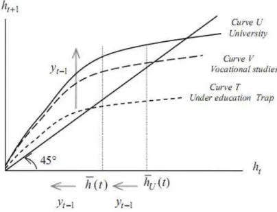
⎠ (15)The three intergenerational dynamics are depicted on Figure 2.
Figure 2. The three intergenerational dynamics
Proposition 2: Consider Educational System
(
τ,qB,qV,qU,λU,eB)
and the set of values{
( )
hˆ ˆi,µi , i=T V U, ,}
µˆi,hˆi ≥0,∑
µˆi =1, qk >0 if µˆk >0,,
k=V U, and such that:
1) hˆT =
(
A yTˆβ)
1/1−η, hˆV =(
A yV ˆ2βµˆV−β)
1/(1−η), and(
2)
1/(1 )ˆ ˆ ˆ
U U U
h = A y βµ −β −η with
(
ˆ ˆ ˆ)
ˆ ˆT T ˆV(1 ˆV) V ˆU(1 ˆU) U
y=ω µ h +µ −e h +µ −e h ;
2) 1/ 2 /(1 ) ˆ ˆ
ˆ (1 ˆ )ˆ ˆ
T
V V V T
k
h h
A e y A y
η
β β β
τ µ − ⎛ − ⎞ ≤ = ⎜⎜ ⎟⎟ − − ⎝ ⎠ ; 3) 1/ ˆ ˆ ˆ U U U T h h A y η β λ ⎛ ⎞
> = ⎜⎜ ⎟⎟
⎝ ⎠ if µˆU >0 ;
4) if both µ µˆV, ˆU >0, then (i)
1 1
ˆ 1 ˆ
ˆ 1 ˆ
U V U V h e e h η − ⎛ − ⎞ ≥ ⎜ − ⎟
⎝ ⎠ and
1/ ˆ
1 ˆ 1
U U U
V V V
e A e A β µ µ ⎛ − ⎞ ≤ ⎜ − ⎟
⎝ ⎠ if
ˆ ˆ
V U
h <h , and (ii)
1 1
ˆ 1 ˆ
ˆ 1 ˆ
U V U V h e e h η − ⎛ − ⎞ = ⎜ − ⎟
⎝ ⎠ and
1/ ˆ
1 ˆ 1
U U U
V V V
e A e A β µ µ ⎛ − ⎞ = ⎜ − ⎟
⎝ ⎠ if
ˆ ˆ
V U
h ≥h .
Then,
{
( )
hˆ ˆi,µi , i T V U= , ,}
define a steady state of Educational System(
τ,qB,qV,qU,λU,eB)
.Proof: Feature (1): hˆT , hˆV and hˆU are respectively the steady states of dynamics (10), (11) and (12). Feature (2) stipulates that all the individuals inside the trap have no interest to pursue vocational studies and Feature (3) that all these who enter the university have enough human capital to do this. Features (4) give the conditions for the dynasties inside V to stay inside V and the dynasties inside V to stay inside V (see the proof in Appendix 5).
Lemma 6: At the steady state, the lifetime income is always lower for the dynasties in segment V than for these in segment U.
Proof: See Appendix 5.
5.2. Possible steady states and resulting segmentations From the dynamics (10)-(12), several features may be identified:
(i) The functions defining the three dynamics being concave, there is a
convergence of the different individuals towards the same human capital level inside each segment T, V and U.
(ii) During the dynamics, certain individuals typically pass from one
segment to another. Consequently, for an initial distribution of human capital across the individuals, there are educational systems that cannot be maintained. This is because, after a number of generations, certain studies disappear as no-one chooses them any longer. Then, the efficiency condition (qi =0 if µi =0, i=V U, ) makes that the initial educational system must be cancelled.
(iii) The long term evolution critically depends on the variation in the
product per capita yt−1. For the individuals who select vocational studies or university, they also depend on the changes in the proportions µV and µU of individuals in each type of study.
The analysis of the different dynamics and of their possible outcomes is described in Appendix 6. These dynamics depend on the values of 2β η+ and β η+ . From this analysis, we derive the following three propositions.
Proposition 3: Assume Educational System
(
τ,qB,qV,qU,λU,eB)
with qi >0, ,i=V U , and education functions such that 2β η+ <1. Then, the human capital dynamics can lead to the following outcomes:
1) Stable Steady states with three segments.
2) Stable steady states with the two segments V and U. 3) A withdrawal of the Educational System.
Proposition 4: Assume an Educational System
(
τ,qB,qV,qU,λU,eB)
and education functions such that 2β η+ =1. Then, the human capital dynamics can lead to:1) A stable steady state if and only if qi =0, ,i=V U
2) A two-group (V and U) permanent segmentation, with the same steady growth rate of the product per capita.
3) A withdrawal of the educational system.
4) Unstable steady states, this outcome being nevertheless very unlikely.
lead to:
1) A stable steady state if and only if qi =0, ,i=V U and β η+ <1
2) If qi =0, ,i=V U and β η+ >1, either a collapse of the economy (i.e. a continuous decrease of human capital and the product per capita), or an unstable steady state, or explosive growth.
3) If qi >0, i=V and / or U, either an unstable steady state, or explosive growth, or a withdrawal of the educational system.
4) In the case of explosive growth with qi >0, ,i=V U, a permanent two-group segmentation with the same growth rates and the same lifetime income in both segments.
6. Simulations
We now implement a series of simulations that illustrate the divergent impacts of different educational patterns upon social segmentation. In this purpose, we apply three educational systems to the same economy. These must not be seen as depicting existing systems but rather as portraying two ideal-types, i.e., one egalitarian system (E) and one inequality-oriented and elitist system (I), and a system in-between (M for medium). The egalitarian system E is pro-education (high public funding), with a rather slight selection and a balanced distribution of taxes across the three courses of study (B, V and U). In the elitist system I, public funding for education is rather low, selection is severe and a substantial part of educational funding goes to a narrow elite. System M is in-between. We start from a certain distribution of human capital and we simulate the intergenerational impact of these three systems.
The egalitarian system results in the disappearing of the under-education trap (i.e., two segments) and in quasi income equality at the steady state. The second system generates three segments with a large under education trap and high inequalities in terms of skill and income. Finally, the third system generates two segments (no trap), quasi equality in the long term, and educational levels that stand in between the two first.
6.1. Initial characteristics and the educational systems parameters
We consider an education function such that 2β η+ <1. This can lead, either to steady states of different shapes (2 or 3 segments), or to the withdrawal from the educational system (Proposition 3).
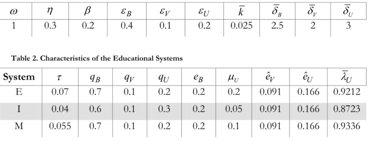
Table 1. The economy's parameters
ω
η β εB εV εU k δB δV δU1 0.3 0.2 0.4 0.1 0.2 0.025 2.5 2 3
Table 2. Characteristics of the Educational Systems
System τ qB qV qU eB µU eˆV eˆU λU
E 0.07 0.7 0.1 0.2 0.2 0.2 0.091 0.166 0.9212
I 0.04 0.6 0.1 0.3 0.2 0.05 0.091 0.166 0.8723
M 0.055 0.7 0.1 0.2 0.2 0.1 0.091 0.166 0.9336
Coefficient η is chosen to correspond to the lower values given by the
estimations of the elasticity of individual skill with respect to the parents’ skill (see Solon, 1999). The parameters εB, εV , εU, k are selected so as to produce results consistent with observed facts in terms of schooling time for each stage of education (8-10 years for basic education, 2-3 years for vocational studies and about 5 years for university) and in terms of fixed cost (Table 1).
The egalitarian system E allocates 7% of total income to education, and its selection procedure is rather slight since it allows 20% of the first generation to enter the university. System E distributes levies between the three types of studies in the proportion qB= 0.7, qV=0.1 and qU= 0.2, i.e. a large proportion of public expenditures allowed for basic education.
The elitist system I allocates 4% of total income to education, restricts the entry to the universities to 5% of the first generation (time 1), and it allows a rather large part of the levies to the universities (30%) at the expense of basic education.
Finally, system M allocates 5.5% of the total income for education, the levies being distributed in the same proportions as in case E with however only 10% of the first generation entering the university because of the selection threshold λU.
It can be noted that these proportions are in line with those observed in Europe and the US, in which (i) public expenditure for education represents between 4-5% of the GDP (Greece, Italy, Spain) and 7-8% (Denmark, Sweden), and (ii) the share of tertiary education in total education expenditure is between 19% (Italy) and 33% (Denmark, Finland)6.
The levels of δB, δV and δU are selected to obtain 70% of the individuals with basic education only, 20% in vocational studies and 10% in the university in the system M at the initial time 1.
We assume a constant number of 1000 dynasties. We start from an initial situation in which 80% of the parents are uniformly distributed over the interval
]
0,1.029]
and 20% are uniformly distributed over the interval]
1.029,1.49746]
. These values are chosen to have a human capital distribution consistent with the European situation in the early seventies.The initial distribution of human capital once determined, the selection thresholds
U
λ for each of the three systems (E, I and M) can be calculated to generate the desired proportion of a generation going to the university at the initial time (see Table 2).
The egalitarian system leads to the following situation at the initial time: 54% of people with basic education only, 26% of people who pursue vocational studies, and 20% of people going to university. In the elitist system, 80% of the population have basic education only, 15% pursue vocational studies and 5% go to university at the initial time. Finally, these proportions are respectively 69%, 21% and 10% in system M.
6.2. The results
Table 3 describes the characteristics of the three steady states, and Figures 3-5 the corresponding human capital dynamics for the 1000 dynasties.
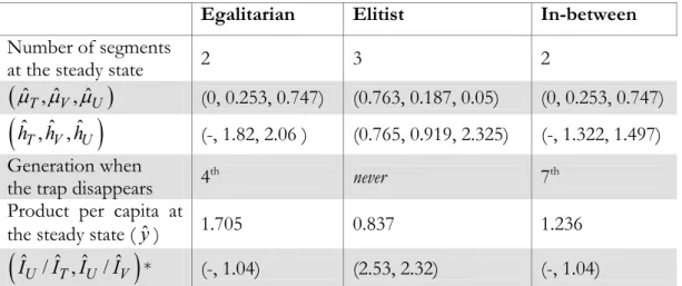
The education trap vanishes in both the egalitarian and the medium systems, at generation 4 for the former and generation 7 for the latter. In contrast, the under education trap is maintained in the elitist system, and it still accounts for 76% of the dynasties at the steady state. Vocational studies and the university respectively represent 25% and 75% of a generation at the steady state in both scenarios E and M, whereas these proportions are 19% and 5% in I. Finally, E and M lead to a quasi equality of the lifetime incomes for all individuals at the steady state (individuals with a university level have a higher human capital than those from vocational studies, but this is almost fully offset by their working time that is lower).
Table 3. The steady states characteristics
Egalitarian Elitist In-between
Number of segments
at the steady state 2 3 2
(
µ µ µˆT, ˆV, ˆU)
(0, 0.253, 0.747) (0.763, 0.187, 0.05) (0, 0.253, 0.747)(
ˆ ,ˆ ,ˆ)
T V U
h h h (-, 1.82, 2.06 ) (0.765, 0.919, 2.325) (-, 1.322, 1.497)
Generation when
the trap disappears 4
th
never 7th
Product per capita at
the steady state (yˆ) 1.705 0.837 1.236
(
ˆ / ˆ ,ˆ /ˆ)
U T U V
I I I I * (-, 1.04) (2.53, 2.32) (-, 1.04)
Figure 3. Segmentation in the Egalitarian educational system (E)
Figure 4. Segmentation in the Elitist educational system (I)
7. Conclusion
We have constructed a stylised model that portrays the main features of educational systems and can be declined in several configurations. We have determined the characteristics of the related possible intergenerational dynamics and shown that the educational system characteristics combined with the initial distribution of human capital across individuals can generate very different social stratifications, with under education traps. This is because individuals from unskilled families attain a low human capital level at the end of basic education, this level being a key factor determining their performance in higher education. They therefore have no incentive to pursue further education because the related cost is higher than the related income benefit. Simulations have finally been implemented to illustrate these findings. The simulations portray two ideal-type systems, one egalitarian and the other elitist, and we also analyse a system in-between. The egalitarian system results in two-segment stratification, quasi income equality and no under education trap whereas the elitist system generates three segments, significant inequality and a large under education trap. This modelling could be extended (e.g., by inserting a larger choice for individuals so as to be closer to reality) and applied to the analysis of the existing systems. In particular, a distinction could be made between Scandinavian systems that provide between 7 and 8% of their GDP for education with a rather large share allocated to higher education and a rather low selection, and Southern European systems allocating 4-5% of their GDP to education, the expenses being centred on primary education. The model can also generate endogenous growth even for 2β η+ <1 if we assume human capital externalities in the production and/or the education function, or by adding an R&D activity that utilises human capital. Finally, the model could be extended to compare the welfare impacts of different educational systems and to analyse public strategies that combine successive educational systems.
References
Anderson C.A. (1961), ‘A skeptical note on the relation of vertical mobility to education’, American Journal of Sociology,66(6), 560-70.
Barham V., Boadway R., Marchand M., Pestieau P. (1995), ‘Education and poverty trap’,
European Economic Review,3, 1257-75.
Baudelot C., Establet R. (1971), L’école capitaliste en France, Paris, Maspero.
Becker G., Tomes N. (1979), ‘An equilibrium theory of the distribution of income and intergenerational mobility’, Journal of Political Economy,87(6), 1153-89.
Becker G., Tomes N. (1986), ‘Human capital and the rise and fall of families’, Journal of Labor
Economics, 4(3), S1-39.
Bénabou R. (1993), ‘Workings of a city: location, education, and production’, Quarterly Journal of
Economics, 108, 619-52.
Bénabou R. (1996a), ‘Heterogeneity, stratification and growth: Macroeconomic implications of community structure and school finance’, American Economic Review,86, 584-609.
Bénabou R. (1996b), ‘Equity and efficiency in human capital investment: The local connection’,
Bertocchi G., Spagat M. (2004), ‘The evolution of modern educational systems. Technical vs. general education, distributional conflict, and growth’, Journal of Development Economics, 73, 559-82.
Bidwell C.E., Friedkin N.E. (1988), ‘The sociology of Education’, in Smelser N. (ed), Handbook
of Sociology, Newbury Park, Sage Publications
Boudon R. (1973), L’inégalité des chances, Paris: Armand Colin. English edition: 1974, Education,
Opportunity, and Social Inequality: Changing Prospects in Western Society, New York,
Wiley-Interscience.
Bourdieu P., Passeron J.-C. (1970), La reproduction. Eléments pour une théorie du système d'enseignement, Paris, Editions de minuit. English edition: 1990, Reproduction in Education, Society and Culture, London, Sage.
Bowles S., Gintis H. (1976), Schooling in capitalist America: Educational reform and the contradictions of
economic life, New York, Basic Books.
Das M. (2007), ‘Persistent inequality: An explanation based on limited parental altruism’, Journal
of Development Economics, 84(1), 251-70.
Driskill R. A., Horowitz A. (2002), ‘Investment in Hierarchical Human Capital’, Review of
Development Economics, 6(1), 48-58.
Durlauf S. (1994), ‘Spillovers, stratification, and inequality’, European Economic Review, 38(3-4), 836-45.
Durlauf S. (1996), ‘A Theory of Persistent Income Inequality’, Journal of Economic Growth, 1, 75-93.
Galor O., Tsiddon D. (1997), ‘The distribution of human capital and economic growth’, Journal
of Economic Growth,2, 93-124.
Galor O., Zeira J. (1993), ‘Income distribution and macroeconomics’, Review of Economic Studies
1993, 60, 35-52.
Kerckhoff A.C. (2000), ‘Transition from school to works in comparative perspective’, in Hallinan M.T. (ed), Handbook of the Sociology of education, New York, Kluwer Academic/Plenum Publishers, 253-74.
Loury G. (1981), ‘Intergenerational transfers and the distribution of earnings’, Econometrica, 49(4), 843-67.
Piketty T. (2000), ‘Theories of Persistent Inequality and Intergenerational Mobility’, in Atkinson A. and Bourguignon F. (eds), Handbook of Income Distribution, Amsterdam, Elsevier.
Shavit Y., Muller W. (2000), ‘Vocational secondary education, Tracking, and social stratification’, in Hallinan M.T. (ed), Handbook of the Sociology of education, New York, Kluwer Academic/Plenum Publishers.
Solon G. (1999), ‘Intergenerational mobility in the labour market’, in Ashenfelter O. and Card D. (eds), Handbook of Labor Economics, 3A, Amsterdam, Elsevier.
Sorokin P. (1959), Social and cultural mobility, Glencoe, IL, Free Press.
Su X. (2004), ‘The allocation of public funds in a hierarchical educational system’, Journal of
Economic Dynamics & Control, 28, 2485-510.
Tavares L.V. (1995), ‘On the development of educational policies’, European Journal of Operational
Research, 82, 409-21.
Thelot C. (1982), Tel père, tel fils. Position sociale et origine familiale, Paris, Dunod.
Appendix 1
Proof of Lemma 4: Individual j prefers V to V if this provides her/him with a higher lifetime income, i.e.
(
)
(
)
ˆ ˆ ˆ ˆ
(1 ) U ( 1) (1 ) V ( 1)
U B U U j V B V V j
wδ δ −e e ε h − η− >f wδ δ −e e ε h − η − f , which gives
after simplifying (1 ˆ )ˆ U (1 ˆ )ˆ V
U eU eUε V eV eVε
δ − >δ − . Identically, the condition for
individual l to prefer V to V is
(
)
(
)
ˆ ˆ ˆ ˆ
(1 ) V ( 1) (1 ) U ( 1)
V B V V l U B U U l
wδ δ −e e ε h − η >wδ δ −e e ε h − η, which gives after
simplifying (1 ˆ )ˆ V (1 ˆ )ˆ U
V eV eVε U eU eUε
δ − >δ − . The coexistence of individuals who
prefer V to V with individuals who prefer V to U is thus impossible. Hence, the coexistence of individuals who select U with individuals who select V is possible in two cases only: (i) if the individuals who select V prefer U but are impeached to enter the university because of threshold λU, and (ii) if, for everyone, choosing U and V
provides the same lifetime earning, which implies (1 ˆ )ˆ U (1 ˆ )ˆ V
U eU eUε V eV eVε
δ − =δ − . In
the later case, the individuals who select V can be or no be constrained by threshold
U
λ for their entry into the university. Thus, when at least one individual who selects V is above threshold λU, U and V must be equally profitable to each individual.
Appendix 2
Proof of Lemma 5: Everyone prefers the university to vocational studies when
, , , ,
ˆ ˆ ˆ ˆ
(1 U) j U (1 V) j V (1 U) j U (1 V) j V,
w −e h − >f w −e h − ⇔ −f e h > −e h ∀j. By inserting
, j U
h and hj V, as defined by (9) into this inequality, it comes: 1/
ˆ
( ) (1 )
ˆ
( ) (1 )
V V V
U U U
t e A
t e A
β
µ ρ
µ
⎛ − ⎞
>⎜ ⎟ ≡ −
⎝ ⎠ . Identically, everyone prefers vocational studies to the
university if µ µV / U<ρ , and both studies are equally profitable if µ µV / U =ρ.
Appendix 3
Reducing the number of individuals inside the under education trap consists in
lowering 1/
(
(1 ) ( (1 ˆ ˆ) V 1))
1/B V V V
h=k η −τ δ δ −e e ε − − η. By inserting (6) and (7) into this expression we obtain:
(
)
1/(
(
)
2(
)
)
1/1/
1 1
ˆ ˆ
(1 ) B (1 ) V ( / )
B B B V V V V V
h k η τ δ e ε βq β η δ e e ε β q µ β τy β τy β η
−
− −
−
− −
= − − − .
The signs of the derivatives are 0
B h q
∂ <
∂ , V 0
h q
∂ <
∂ , 1 0
h y−
∂ <
∂ and 0
h k
∂ >
∂ . In
Appendix 4
From
(
)
(
)
1/ 1/ / ) / 1/ 1 ( / B UU U B
B B B
h
e q y
η η β η β η η ε λ λ δ
δ − τ −
= = , it is clear that
0 U U h λ ∂ >
∂ , UB 0
h q
∂ <
∂ , ∂hU /∂ <τ 0 and ∂hU /∂y−1<0.
Appendix 5
Proof of Feature (4) of Proposition 2: As hˆV =
(
A yV ˆ2βµˆV−β)
1/(1−η) and(
2)
1/(1 )ˆ ˆ ˆ
U U U
h = A y βµ −β −η (Proposition 2, feature 1), then
1/(1 )
ˆ ˆ
ˆ ˆ
V V U
U V U h A A h η β µ µ − ⎛ ⎛ ⎞ ⎞ ⎜ ⎟ = ⎜ ⎟ ⎜ ⎝ ⎠ ⎟ ⎝ ⎠ .
The dynasties inside segment V remain in V and those inside U remain in U in two cases:
1) when hˆV <hˆU <hˆU and
( )
( )
2 2
1 ˆ 1 ˆ
ˆ ˆ ˆ ˆ
(1 U) U t U i (1 V) V t V i
w −e A y− βµ −β h η− ≥f w −e A y− βµ −β h η− f , i = V,U, i.e.,
ˆ ˆ
1
ˆ ˆ
1
U V U
V U V
e A e A β µ µ ⎛ ⎞ − ≥ ⎜ ⎟
− ⎝ ⎠ , and thus
1/(1 )
1/(1 )
ˆ ˆ 1 ˆ
ˆ ˆ 1 ˆ
V V U U
U V V
U
h A e
A e h η β η µ µ − − ⎛ ⎛ ⎞ ⎞ ⎛ − ⎞ ⎜ ⎟ = ⎜ ⎟ ≤⎜ ⎟ − ⎜ ⎝ ⎠ ⎟ ⎝ ⎠ ⎝ ⎠ .
2) when hˆV >hˆU and selecting V or U is indifferent for both the individuals in V
and U, i.e. w(1−eˆU)A yU t−12βµˆU−β
( )
hˆi η =w(1−eˆV)A yV t−12βµˆV−β( )
hˆi η, i=V U,(Lemma 4), i.e., 1 ˆ ˆ
ˆ ˆ
1
U V U
V U V
e A e A β µ µ ⎛ ⎞ − = ⎜ ⎟
− ⎝ ⎠ , and thus
1/(1 )
ˆ 1 ˆ
ˆ 1 ˆ
V U V U h e e h η − ⎛ − ⎞ = ⎜ − ⎟ ⎝ ⎠ .
Inequality w(1−eˆU)A yU t−12βµˆU−β
( )
hˆi η ≥w(1−eˆV)A yV t−12βµˆV−β( )
hˆi η alwaysholds, and thus: 1 ˆ ˆ
ˆ ˆ
1
U V U
V U V
e A e A β µ µ ⎛ ⎞ − ≥ ⎜ ⎟ − ⎝ ⎠ .
Proof of Lemma 6: The steady state lifetime income is lower for the dynasties in segment V than for these in segment U if and only if (1−eˆU)hˆU > −(1 eˆV)hˆV. In all
cases we have (see above): 1 ˆ ˆ
ˆ ˆ
1
U V U
V U V
e A e A β µ µ ⎛ ⎞ − ≥ ⎜ ⎟
− ⎝ ⎠ . Since
1/(1 )
ˆ ˆ
ˆ ˆ
V V U
1/(1 )
ˆ 1 ˆ
ˆ 1 ˆ
V U V U h e e h η − ⎛ − ⎞ ≤ ⎜ − ⎟
⎝ ⎠ , and after rearranging
/(1 ) ˆ
ˆ ˆ
(1 ) 1
ˆ 1 ˆ
ˆ
(1 )
V V U
V
U U
e h e
e e h
η −η
⎛ ⎞
− −
≤ ⎜ − ⎟
− ⎝ ⎠ , with
/(1 ) ˆ 1 1 ˆ 1 U V e e
η −η ⎛ − ⎞
< ⎜ − ⎟
⎝ ⎠ since 1>eˆU >eˆV. Hence
ˆ ˆ
ˆ ˆ
(1−eU)hU > −(1 eV)hV.
Appendix 6
Equations (10)-(12) and Figure 2 in the text describe the dynamics of the dynasties depending on their segment (T, V, or U). In each of the possible three segments, the individual dynamics converge towards the same human capital level. To analyse the different possible outcomes of these dynamics, let us suppose that all the dynasties belonging to one segment have the same human capital at each period of time (this human capital changing with time). Assuming this, there are three dynamics only which are as follows:
• For the dynasties inside the under education trap:
(
)
1
( ) ( 1)
T t T t T t
h =A y− β h − η (A1)
• For the dynasties following vocational studies:
(
) (
)
2 1
( ) ( ) ( 1)
V t V t V t V t
h =A y− β µ −β h − η (A2)
• For the dynasties having a university degree:
(
) (
)
2
1 ( )
( ) ( 1)
U U t U t U
h t = A y− β µ −β h t− η (A3)
with:
(
)
1 ( 1) ( 1) (1 ) ( 1) ( 1) (1 ) ( 1) ( 1)
t T t T t V V t V t U U t U t
y− =ω µ − h − + −e µ − h − + −e µ − h − (A4)
By inserting (A4) into (A1)-(A3), and after rearranging, it comes:
(
)
1( 1) ( 1)
( )
( 1)
( 1) ( 1)
V V U U
T
T T T
T T
t t
t
t
t t
a h a h
h
B a h
h h
β
η β+ −
− −
−
− −
⎛ + ⎞
= ⎜ + ⎟
⎝ ⎠ (A5)
(
)
2
2 1
( 1) ( 1)
( 1) ( 1)
( )
( 1)
V T T U U
V V V
V V
t t
t t
t
t
h a h a h
B a h
h h
β
β η+ −
− −
− − −
⎛ + ⎞
= ⎜ + ⎟
(
)
22 1
( 1) ( 1)
( 1) ( 1)
( )
( 1)
U T T V V
U U U
U U
t t
t t
t
t
h a h a h
B a h
h h
β
β η+ −
− −
− − −
⎛ + ⎞
= ⎜ + ⎟
⎝ ⎠ (A7)
with BT = ATωβ , BV = AVω2β
(
µV( )t)
−β, BU =AUω2β(
µU( )t)
−β ,( 1)
T T t
a =µ − , aV = −(1 eˆV)µV(t−1), and aU = −(1 eˆU)µU(t−1). Combining (A2) and (A3) yields:
( ) ( 1)
( ) ( 1)
V V V
U U U
t t
t t
h B h
h B h
η
− −
⎛ ⎞
= ⎜ ⎟
⎝ ⎠ (A8)
From (A8), it is clear that hV( ) /t hU( )t tends towards the steady value
(
)
1/1/
V U
B B −η. Hence, any steady state is such that:
1 1
1
1 1
ˆ ˆ ˆ
ˆ ˆ ˆ
V
U
V V V V V U
U V
U U U U
h B e q
B
h e q
β
ε β β η
η η
ε β β
δ µ µ δ − − − − − ⎛ ⎞ ⎛ ⎞ ⎛ ⎞ =⎜ ⎟ = ⎜⎜ ⎟⎟ ⎜ ⎟
⎝ ⎠ ⎝ ⎠ ⎝ ⎠ (A9)
In addition, suppose that at the steady state the dynasties in segment V are not constrained by the barrier to entry in the university, i.e. hˆV ≥hˆU. Then, we know from
Proposition 2 that
1/(1 )
ˆ 1 ˆ
ˆ 1 ˆ
U V U V h e e h η − ⎛ − ⎞ = ⎜ − ⎟
⎝ ⎠ and
1/ ˆ
1 ˆ 1
U U U
V V V
e A e A β µ µ ⎛ − ⎞ = ⎜ − ⎟
⎝ ⎠ . Relations
(A5)-(A7) form a three-equation dynamic system that depends on the values 2β η+ and β η+ .
1) First case: 2β η+ <1. As 2β η+ − <1 0, functions (A5)-(A7) are respectively decreasing in hi(t−1), , ,i=T V U. The possible outcomes of these dynamics are
depicted on Figures A1.
In Cases (a) and (b), the dynamics result in three-segment steady states (hˆT <hˆ). In the case (a), certain dynasties would select the university if they were not prevented for this by the level of the barrier to entry (hˆV <hˆU). As a consequence, for the values
ˆ V
h and hˆU, selecting the university would provide higher earnings to the individuals in
V and
1/ ˆ
1 ˆ 1
U U U
V V V
e A e A β µ µ ⎛ − ⎞
< ⎜ − ⎟
⎝ ⎠ (Proposition 2). In case (b), the dynasties who select