Sex-Specific Selection and Sex-Biased Gene
Expression in Humans and Flies
Changde Cheng, Mark Kirkpatrick*
Department of Integrative Biology, University of Texas, Austin, Texas, United States of America
Abstract
Sexual dimorphism results from sex-biased gene expression, which evolves when selection acts differently on males and females. While there is an intimate connection between sex-biased gene expression and sex-specific selection, few empirical studies have studied this relationship directly. Here we compare the two on a genome-wide scale in humans and flies. We find a distinctive “Twin Peaks” pattern in humans that relates the strength of sex-specific selection, quantified by genetic divergence between male and female adults at autosomal loci, to the degree of sex-biased expression. Genes with intermediate degrees of sex-biased expression show evidence of ongoing sex-specific selection, while genes with either little or completely sex-biased expression do not. This pattern apparently results from differential viability selection in males and females acting in the current generation. The Twin Peaks pattern is also found inDrosophilausing a different measure of sex-specific selection acting on fertility. We develop a simple model that successfully recapitulates the Twin Peaks. Our results suggest that many genes with intermediate sex-biased expression experience ongoing sex-specific selection in humans and flies.
Author Summary
Sexual dimorphism, which is evident in virtually all phenotypic traits, results from sex-biased gene expression. The evolution of sex-biased expression, in turn, results from selection that acts differently on males and females. We use genomic data from humans and flies to quan-tify the relation between ongoing selection pressures and gene expression. A distinctive pat-tern in both species reveals that many genes are experiencing selection that is currently acting differentially on males and females. These results suggest that the “war between the sexes” is more than a metaphor: it contributes to observable patterns of mortality in humans.
Introduction
Females and males differ for virtually all phenotypic traits [1]. Sexual dimorphism results from sex-biased gene expression, which evolves in response to selection that acts differently on males and females [2–4]. Thus sex-biased gene expression is intimately linked to sex-specific
a11111
OPEN ACCESS
Citation:Cheng C, Kirkpatrick M (2016) Sex-Specific Selection and Sex-Biased Gene Expression in Humans and Flies. PLoS Genet 12(9): e1006170. doi:10.1371/journal.pgen.1006170
Editor:Michael W. Nachman, University of California, Berkeley, UNITED STATES
Received:March 15, 2016
Accepted:June 14, 2016
Published:September 22, 2016
Copyright:© 2016 Cheng, Kirkpatrick. This is an open access article distributedunder the terms of the
Creative Commons AttributionLicense, which permits unrestricteduse, distribution,and reproduction in any medium, provided the original author and source are credited.
Data Availability Statement:All data used in this study were downloadedfrom public repositories, specifically:human SNP data:http://www. 1000genomes.org/data#download, human expression data:http://www.gtexportal.org/home/, and fly expression data:http://www.ncbi.nlm.nih.gov/ geo/query/acc.cgi?acc=GSE17013.
selection [5,6]. What is less clear, however, is the extent to which sex-specific selection is ongo-ing, and how ongoing selection relates to the strength of sex-biased expression.
To date, the most direct link between sex-specific selection and sex-biased expression comes from a laboratory study ofDrosophila melanogaster. By comparing gene expression and repro-ductive fitness in a quantitative genetics design, Innocenti and Morrow [7] identified genes experiencing sexually-antagonistic selection, which is the extreme case of sex-specific selection in which an allele that increases fitness in one sex decreases it in the other. They concluded that 8.5% of loci that show sex-biased expression are experiencing ongoing sexually-antagonistic selection. While this work is a milestone, it leaves key questions unanswered. These include: What is the relation between the strength of ongoing sex-specific selection and sex-biased expression, and how common and how strong is sex-specific selection in natural populations? Answers to these questions are important to our understanding of how sexual dimorphism evolves. Further, the answers will inform us about general issues including constraints to adap-tation [8–10] and how genomes evolve [11–13].
We tackle this problem here with a new method that directly quantifies contemporary sex-specific selection on a genomic scale. We reason that Mendelian inheritance ensures that allele frequencies at autosomal loci are equal in males and females at conception, and that sex-spe-cific viability selection will generate genetic divergence between the sexes within a generation. Divergence will occur when selection is sexually-antagonistic, meaning that different alleles are favored in males and females. Divergence also results when selection of different strengths favors the same allele in males and females, a situation sometimes called “sexually-concordant selection” [14]. We use the term “sex-specific selection” here to include both cases.
We find that genes with intermediate degrees of sex-biased expression experience the stron-gest sex-specific selection in humans. We assess the generality of this pattern by reanalyzing the data on flies from Innocenti and Morrow [7]. We again find the The Twin Peaks pattern, which in this case results from sexually-antagonistic (not sexually-concordant) selection, and from selection on fertility (rather than viability). A simple population-genetic model success-fully recapitulates the key pattern. Our results suggest that ongoing sex-specific selection is a common feature of the genome in humans and flies.
Results
Sex-specific selection and sex-biased expression in humans
We quantify sex differences in viability selection usingFSTbetween adult males and females [15]. We used allele frequencies at over 6 million autosomal single-nucleotide polymorphisms (SNPs) that appear in the 1000 Genomes Project [16], a database that includes more than 2000 individuals from 26 populations worldwide. For each of 17,839 protein-coding loci, we calcu-lated the averageFSTfor all SNPs within transcribed regions within each population. We expect this to give a conservative picture of sex differences in selection since most SNPs are not them-selves targets of selection. Rather, they change frequency through hitchhiking, and theFSTthat results at these SNPs is expected to be less than that at a selected SNP in the same gene. Patterns that are qualitatively the same as what we report below also emerge if we use only the single SNP from each locus with the largest value ofFST. No SNP showed significantly different allele frequencies in males and females at a false discovery rate of 5%. That is not surprising, how-ever. A power analysis presented in theS1 Fileshows it is highly unlikely to observe significant divergence at any individual SNP, even with very strong sexually-antagonistic selection, simply because the correction for multiple comparisons is so severe.
We quantify sex-biased expression as the normalized difference between expression in males and females:Δ= (m–f) / (m+f), wheremandfare the transcript abundances in males
and females. (This measure is highly correlated with the familiar log2of the expression ratio.)
A value ofΔ= –1 means a gene is expressed only in females,Δ= 0 means expression is unbi-ased, andΔ= 1 means it is expressed only in males. We use RNAseq data from the Genotype-Tissue Expression Project [17]. Sex-biased expression in adults mainly results from differences between reproductive tissues [18,19], so we used expression levels in testis and ovaries. The data are from 14 males and 6 females [20].
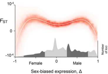
We find that genetic divergence between males and females is related to the degree of sex-biased expression by a distinctive pattern that we call “Twin Peaks” (Fig 1). AverageFST
reaches a minimum when expression is unbiased (Δ= 0). Genetic divergence between the sexes is greatest for genes whose expression is moderately female-biased D 1
2
or moderately
male-biased D1
2
. After reaching these peaks, genetic divergence then declines again as expression tends towards complete female-bias (Δ= –1) and complete male-bias (Δ= 1).
The Twin Peaks pattern is statistically well-supported. The best fit regression ofFSTonΔis a fourth-degree polynomial with two peaks (S1 Table). We permutated the data 105times and found the pattern occurs 1.6% of the time (that is, the pattern is significant atp= 0.016, details inMaterials and Methods). The Twin Peaks pattern is also recovered by fitting a cubic spline using generalized additive models. Twin Peaks are seen within each of the 26 populations when they are analyzed separately. Genetic divergence between the sexes is quite repeatable across populations: taking the SNP with highestFSTat each locus, the intra-class correlation coefficient is 0.34. Finally, the Twin Peaks also emerge when we measure genetic divergence between the sexes using the statisticDainstead ofFST[21,22] (S2 Table,S3 Fig).
It is plausible that gene expression in adult gonads (on which our analyses are based) is not itself the target of the viability selection that causes the Twin Peaks pattern. Instead, expression in adult gonads could be correlated with expression in other tissues and other life stages that are the actual targets. Unfortunately, we are not able to repeat our analyses with most somatic tissues because the Gene Expression Atlas only provides data on expression averaged across both sexes. We were however able to analyze expression in five sex-specific somatic tissues: ectocervis, fallopian tubes, vagina, and uterus in females, and prostate in males. The Twin Peaks pattern appears again when we use the average expression of the four female-specific Fig 1. The strength of sex-specific selection is strongest on human autosomal genes with
intermediate sex-biased expression.The white curve is the best-fit 4thdegree polynomial and the intensity
of red indicates the likelihood that the regression passes through a given value. The averageFSTfor the
SNPs in a gene is small atΔ= 0 (unbiased expression), increases to a peak as sex-bias grows, then decreases asΔapproaches –1 and 1. The numbers of genes with a given bias are visualized in the density plot in the lower part of the figure; dark gray denotes intermediate sex-biased expression.
somatic tissues and expression in testes, but not when we use prostate instead of testes. Expres-sion in prostate may not provide a good proxy for gene expresExpres-sion in males, however, as its expression profile is very similar to that of vagina and other female-specific tissues [20].
Sex-specific selection could be acting on regulatory elements as well as coding regions. We therefore repeated the analyses including all noncoding transcripts whose expression is profiled in the Genotype-Tissue Expression Project (34,060 in total) and the 1kb sequence upstream of all coding regions used in the previous analysis. Once again, a significant Twin Peaks pattern appears.
We considered the possibility that the pattern is driven by heterozygosity. Imagine that the strength sex-specific selection does not vary systematically with sex-biased expression, but that heterozygosity follows the Twin Peaks pattern. Then genetic divergence between males and females, measured asFST, will also show that pattern. (This prediction follows because changes in allele frequencies caused by selection are proportional to heterozygosity.) We therefore regressed the quantity (FST/pq) ontoΔ, wherepandqare the frequency of the two alleles at a given SNP. If the Twin Peaks results from variation of heterozygosity with sex-biased expres-sion, the regression is expected to be flat. This alternative hypothesis is falsified: Twin Peaks are again seen using the polynomial and spline regressions described above (S3 Table). We also fit a regression model that included both heterozygosity andΔas factors. The Twin Peaks pattern remains significant (p<0.01) even after the effect of heterozygosity onFSTis controlled for.
While no individual SNP showed significantFSTbetween the sexes, the identities of several highly diverged genes do hold hints of possible connections to sex-specific selection. The gene
RNF212segregates for alleles that have opposing effects on male and female recombination rates [23,24]. The meanFSTfor the SNPs in this gene is in the top 0.2% of all the loci we ana-lyzed. Other genes in the top 5% ofFSTvalues are two loci (LYPLAL1andADAMTS9) associ-ated with the waist-hip ratio [25]. This is a sexually-dimorphic phenotype that has long been associated with sexual attractiveness [26]. A recent review identified 33 loci that have been linked by multiple genome-wide association studies to sex-specific risk of disease [27]. The most diverged SNPs at these genes haveFSTvalues that are significantly higher than average (p<4 x 10⁻⁵by a permutation test). A final observation is that a set of genes that show evi-dence of balancing selection [28] also haveFSTvalues that are significantly higher than the genome-wide average (p<1 x 10⁻⁶by a permutation test). This correlation could result if sexu-ally-antagonistic selection itself is maintaining polymorphism at these loci [29], or if sex-spe-cific selection acts on polymorphisms that are maintained by other mechanisms (e.g. overdominance).
These results lead us to conclude that the Twin Peaks pattern in humans results from sex-specific viability selection whose strength varies with the degree of sex-biased gene expression.
Twin Peaks also occur in flies
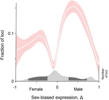
To test the generality of the pattern we discovered in humans, we reanalyzed the fly data from Innocenti and Morrow [7]. Here our measure of the strength of sex-specific selection acting on a locus is binary: it takes a value of 1 if they identified it as a target of sexually-antagonistic selection, and is 0 otherwise. Their data are based on fertility selection, rather than viability selection. We again quantified sex-biased gene expression usingΔbased on their transcriptome data. We then asked if fraction of genes under sexually-antagonistic selection varies systemati-cally withΔ.
when it is completely sex-biased (Δ= –1 or 1). The pattern is highly statistically significant (p<10−5) by bootstrapping using regressions based both on polynomials and splines (see Materials and Methods).
The pattern in flies is consistent with that in humans. A difference between the two data sets is that the pattern in humans results from genetic effects on viability, while the pattern in flies reflects effects on fertility and fecundity. Together, these results suggest that a tendency for stronger sex differences in selection to act on genes with intermediate sex-biased expression may be general to diverse forms of selection.
A simple model explains Twin Peaks
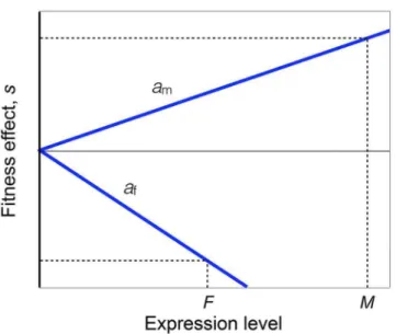
To understand the Twin Peaks pattern, we built a simple model that relates gene expression to fitness. Three key assumptions are invoked: (1) Allele frequencies are at equilibrium under sex-ually-antagonistic viability selection, which is the special case of sex-specific selection in which selection favors one allele in one sex and the other allele in the other sex; (2) A gene that is not expressed experiences no selection; and (3) At low expression levels, the effects of alleles on via-bility increase approximately linearly with the amount of expression. These assumptions are illustrated graphically inFig 3. The model allows selection to be frequency-dependent, and for arbitrary dominance. Further details and the analysis of the model are given in the Materials and Methods section.
This model leads to two predictions regarding how genetic divergence between the sexes varies with the degree sex-biased expression. First, we find that whenΔis near to 0,
FST4p q amaf amþaf
!2
D2; ð1Þ
whereamandafmeasure how the strength of selection varies with the gene’s expression in Fig 2. The Twin Peaks pattern in flies.The relation between the fraction of genes under
sexually-antagonistic selection andΔis shown by the best-fit cubic spline (white line), and the 95% confidence interval is shown by the shaded areas. The distribution of gene numbers is shown at the bottom of the figure.
males and females (seeFig 3). We see that allele frequency divergence between the sexes depends on three kinds of quantities: heterozygosity (proportional to 4pq), the potential for sexually-antagonistic selection (represented by the term in parentheses), and the strength of sex-biased expression (represented byΔ).
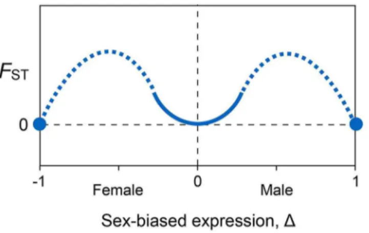
All else equal, this result predicts thatFSTwill be 0 when expression is unbiased, and it will increase quadratically as expression becomes slightly female- or male-biased. Second, the model predicts thatFSTwill also be zero when expression is completely female-biased and completely male-biased. The model does not apply to genes whose expression is strongly but not completely sex-biased. We can, however, make qualitative predictions for these cases by interpolating between the predictions from the first two cases. The pattern that results is Twin Peaks (Fig 4).
To check the qualitative fit of this model to data, we focused on genes in the human dataset whose expression is weakly sex-biased. We took all genes expression lies between the two peaks atΔ= –0.52 andΔ= 0.72, which includes 80% of the genes in the dataset. The best-fit polyno-mial regression is a quadratic with a significantly positive coefficient (p<<0.001), as predicted by our model (S4 Table). In principle, we might use the curvature of this regression to estimate the quantity that appears within parentheses inEq (1). That would be of interest because it is a measure of the potential for sexually-antagonistic selection. We do not take that step here, however, because as we now explain these data may not be adequate to give accurate estimates of selection.
The strength and prevalence of sex-specific selection in humans
Under the assumptions of our model, the value ofFSTbetween males and females is propor-tional to the strength of sexually-antagonistic viability selection (seeMaterials and Methods). This suggests that one might estimate the strength of sexually-antagonistic selection from these Fig 3. Schematic of the genetic model.The X-axis shows the expression of a locus, measured as the log of the number of transcripts, in males (M) and females (F). The Y-axis shows the additive fitness effect of an allele in males (sm) and females (sf). No selection (sm,sf= 0) occurs when there is no expression (M,F= 0).Fitness effects increase with expression at a rateamin males andafin females. At an evolutionary
equilibrium,sm= –sf. Our measureΔof sex-bias is approximately equal to twice the difference betweenM
andF, normalized by the total of expression in both sexes,M+F, whenΔis small. Further details are given in the Materials and Methods section.
data. Using the averageFSTfor a gene biases the estimate downward because the large majority of SNPs are not expected to be direct targets of selection. Using the SNP in a gene with the larg-estFST, on the other hand, biases estimates upward because this extreme value is expected to result partly from sampling variance.
With these caveats in mind, we attempted to make a rough estimate for the strength of sexu-ally-antagonistic selection acting on genes with intermediate sex-biased expression (see Materi-als and Methods). Focusing on the YRI population (Yoruba in Ibadan, Nigeria) because it is the most genetically variable, we sampled loci whose values ofΔfall close to maxima of the two Twin Peaks and whose values ofFSTare close to the average for genes with that degree of sex-biased expression. Using the averageFSTfor all the SNPs in each gene, we estimate that the additive fitness effects of alleles at these loci ares= 0.02 on average. If correct, this result would suggest that sexually-antagonistic selection at these loci is strong. The estimate is based on small numbers of individuals, however, and so it is imprecise. The estimate is also likely to be biased upwards, as we will see shortly.
What fraction of genes experiences sex-specific selection in humans? While it is difficult to quantify that number with precision, we can get a crude idea by summing the number of loci that lie beneath the Twin Peaks, for example those whose sex-biased expression lies between 0.25<|Δ|<0.75. In both humans and flies, those are about 40% of coding genes. These results suggest that sex-specific selection could be common in both species.
The selection load
Sex differences in autosomal allele frequencies between mature females and males result from differential survival after conception. Unlike other kinds of genetic load [30], this engenders a true mortality load on the population. We can calculate this load under the assumption of our model that the loci are at equilibrium under sexually-antagonistic selection in which an allele that increases viability in one sex decreases it in the other (seeMaterials and Methods). The additional mortality incurred by a population due to sexually-antagonistic selection on a single locus with additive effects is simplyLSA=s, wheresis the fitness effect of an allele (positive in one sex, negative in the other). This result suggests that not many loci can be under strong sex-ually-antagonistic selection or the population would not be viable. For example, sexually-Fig 4. Qualitative conclusions from the genetic model.Genetic divergence between the sexes, measured asFST, is minimized when gene expression is unbiased (Δ= 0), then increases quadratically for small
degrees of female-biased and male-biased expression (solid curve).FSTis also 0 when expression is
completely female-biased (Δ= –1) or male-biased (Δ= 1) (solid circles). Values ofFSTexpected for
intermediate sex-dependent expression are interpolated by eye (dashed curves).
antagonistic acting on 100 loci with independent fitness effects ofs= 0.01 reduces the average viability in the population by 63%.
This consideration argues that the estimates for the strength and prevalence of selection offered in the previous section may be substantial overestimates. Factors that may contribute are discussed below.
Discussion
This study focuses on the relation between the strength of ongoing sex-specific selection to the degree of sex-biased expression. In humans, we used allele frequencies at 6 million coding SNPs sampled from 26 populations. We quantify the strength of sex differences in selection acting within a generation usingFSTbetween males and females adults. In flies, we quantified specific selection as the fraction of loci that had been previously identified as targets of sex-ually-antagonistic selection [7]. In both species, we see a distinctive Twin Peaks pattern in which sex-specific selection is strongest for genes with intermediate sex-biased expression, and is weak when bias expression is either complete or absent. These results suggest that sex-specific selection is ongoing at many genes. We develop a simple genetic model that recapitu-lates the Twin Peaks pattern.
In a recent study, Lucotteet al. [31] used theFST-based strategy that we employed to scan the HapMap dataset [32] for SNPs with divergent allele frequencies in males and females. Under their most stringent statistical criteria, they found two X-linked loci that are significantly diverged (at a FDR of 5%). (Those loci do not appear in our analyses because we excluded the sex chromosomes.) Further, they reported that extremeFSTvalues are enriched on the X chro-mosome relative to the autosomes, consistent with what is expected from sexually-antagonistic selection. Taken together with our results from the 1000 Genomes dataset, the consistent pic-ture is that there is evidence of ongoing sex-specific selection in humans.
Other processes besides sex-specific selection might contribute to the sex differences in allele frequencies we observed in humans. Population structure can generateFSTbetween the sexes. If populations have different allele frequencies, then differential migration of one sex will generateFSTbetween the sexes within a population.FSTbetween the sexes will also appear in the data if viability selection acts equally on males and females but the sexes are sampled at dif-ferent ages.
It seems unlikely, however, that these alternative hypotheses explain the Twin Peaks pattern. While both population structure and age differences can inflateFSTbetween the sexes in the human dataset, it is difficult to see how either of those factors would generate a pattern that varies systematically with sex-biased expression. Further, neither population structure nor age differences are factors in the fly dataset. Sex-specific selection therefore appears to be strongly supported.
As we noted in the Results, it is plausible that the Twin Peaks pattern does not result from viability selection on gene expression in adult gonads (which is what our analysis is based on), but rather from selection on correlated traits such as expression in other tissues and/or at other ages. If so, we expect that our results are conservative: the pattern we observed is weaker than what would be seen if divergence in male and female allele frequency was regressed against the true targets of selection.
could be substantially lower. Unfortunately, it does not seem possible to estimate the strength of selection from our data under these more general conditions. Further, as we discussed ear-lier, geographical and age structure in the data may contribute to the genetic differences between the sexes.
The fly data also include biases. One results from sex differences in the allometry of body parts. Innocenti and Morrow [7] measured gene expression in the whole bodies of flies. Differ-ences in transcript abundances between tissues that have different relative sizes in males and females will result in sex differences in relative expression, and so bias ourΔstatistic. It is diffi-cult, however, to see how this bias would vary systematically with the fraction of genes under sexually-antagonistic selection and so produce the Twin Peaks pattern.
Our model suggests that the Twin Peaks pattern is expected to emerge under certain condi-tions. Two in particular deserve consideration. The first assumption is that selection is sexu-ally-antagonistic, with different alleles favored in males than in females. OurFST-based analysis of the human data is not able to discriminate between sexually-antagonistic selection and sexu-ally-concordant selection (when the same allele is favored with different strengths of selection in males and females). We note, however, that the Twin Peaks pattern in flies does result from sexually-antagonistic (and not sexually-concordant) selection. Second, the model assumes that allele frequencies are at equilibrium. Unfortunately, we are unable to generalize either of these two assumptions. But while the quantitative results from the model will not hold if those assumptions are violated, it seems likely that the Twin Peaks pattern will emerge under a broader range of conditions than our model assumes.
Our results and those of Innocenti and Morrow [7] suggest that a substantial number of genes are targets of ongoing sex-specific selection. Why hasn’t evolution adjusted expression levels and resolved this tension? Two general ideas have been offered. One is that pleiotropy is extensive and so there is little genetic variation available to decouple expression levels in males and females [2,33–36]. A second suggestion is that selection pressures may fluctuate over time and space, and evolutionary lags prevent the degree of sex-biased expression from being opti-mized in the current environment [37–39]. This hypothesis is consistent with the high turnover rate seen of genes with sex-biased expression [19,40–42].
The holy grail of evolutionary genomics has been to identify individual genes that underlie adaptation. Our approach shows that even when that goal is not possible, we can nevertheless make important inferences about selection and adaptation by studying genome-wide patterns. The strategy of combining data across genes with a simple model has offered a new perspective on the evolution of sex-biased gene expression. Similar strategies may also be fruitful in studies of other problems.
Materials and Methods
A simple model relating
FST
between the sexes to sex-biased gene
expression
Allele frequencies at autosomal loci are equal in males and females among zygotes. Sexu-ally-antagonistic selection acting on viability will cause divergence in allele frequencies between adult males and females. Consider a locus segregating for allelesAanda. To measure the impact of sexually-antagonistic selection, we use the familiarFSTstatistic:
FST ¼
ðpm pfÞ
2
4p q ; ð2Þ
wherepmandpfare the frequencies ofAin mature males and females,pis its frequency in zygotes, andq= 1 –p.
Write the relative viabilities of genotypesaa,Aa, andAAin males as 1:: 1 +hmSm::Sm. The selection coefficientSmand dominance coefficienthmcan be frequency-dependent, in which case these coefficients take their values at equilibrium (see below). Assuming that zygotes are at Hardy-Weinberg equilibrium, the allele frequency in adult males is
pmpþpq sm; ð3Þ
wheresmis the additive itness effect of alleleAin males, deined as
sm¼ ½pþ ðq pÞhmSm: ð4Þ
The approximation ofEq (3)neglects terms of orders2
m. An analogous expression gives the
additive itness effect of alleleAin females,sf. The divergence between males and females is
therefore
FST
1
4pqðsm sfÞ
2
: ð5Þ
We link selection to expression by assuming that when expression is low, the fitness effects can be approximated by the functions:
sm¼amM
sf ¼afF;
ð6Þ
where
M¼lnðmþ1Þ
F¼lnðfþ1Þ; ð7Þ
andmandfare the absolute expression levels (e.g. number of transcripts per cell or in a tissue). The coeficientsamandafrelect how sensitive selection is to the expression level. At a locus under sexually-antagonistic selection, these coeficients have opposite signs. The situation is sketched inFig 3.
Eqs (6and7) have three desirable features. First, the fitness effect of an allele in a given sex is 0 if the gene is not expressed in that sex. Second, for values ofmandfmuch larger than 1, changes in transcript abundance have proportional effects on the strength of selection. For exam-ple, a 10% increase in expression has the same effect on fitness regardless of whether there are 100 or 1,000 transcripts in the cell. Last, we will see below that the logarithmic scaling for expres-sion used inEq (7)leads to predictions from the model that can be directly compared to data.
is frequency-dependent.) The equilibrium condition andEq (6)imply that
T¼ af am
af þam
!
D; ð8Þ
whereTis the total expression andDis the difference in expression (sex-bias) between males and females:
T ¼MþF
D¼M F: ð9Þ
Substituting Eqs (6–9) intoEq (5)gives
FST p q A D
2; ð10Þ
where
A¼ amaf
amþaf
!2
: ð11Þ
Eq (10)gives a pleasingly simple relationship between the divergence of allele frequencies between the males and females resulting from sexually-antagonistic selection, on the one hand, and the degree of sex-biased expression, on the other. Three quantities appear on the right side. First is the termpq, which is proportional to heterozygosity. The second isA, which is a mea-sure of the potential for sexually-antagonistic selection. Last isD2, which is the square of the sex-bias in expression.
We want to express these results in terms of quantities that have been estimated. A natural measure of sex-biased is
D¼m f
mþf; ð12Þ
wheremandfare the transcript abundances in males and females. The measureΔis 0 when expression is unbiased, reaches a minimum value ofΔ= −1 when a gene is expressed only in females, and a maximum value ofΔ= 1 when it is expressed only in males. When bias is small and the absolute expression levels are much greater than 1, a Taylor expansion shows that
D1
2ln
m f
1
2D: ð13Þ
SubstitutingEq (13)intoEq (10), we finally have
FST4p q AD
2
; ð14Þ
which appears asEq (1)in the main text.
To summarize, our model makes three predictions:FSTwill be 0 for a gene with unbiased expression (Δ= 0), it will increase quadratically withΔfor small amounts of male- and female-biased expression, and finally it will return to 0 for a gene that are expressed only in females or in males (Δ= −1 andΔ= 1). The results are shown graphically inFig 4.
The strength of sexually-biased selection
We estimated the strength of selection from the frequencies of alleles in females and males. Fol-lowing the notations and assumptions described in previous sections, we assume that loci under sexually-antagonistic selection and are at equilibrium. That implies that the fitness effect of an allele in females is equal in magnitude and opposite in sign to its effect in males. The total numbers of alleles sampled from females and males are denotedNfandNm, and the numbers of the minor allele observed arenfandnm. We assume the samples are independent.
Denote the (unknown) frequency of the minor allele in zygotes at a given locus asp. Then likelihood ofsm, the additive fitness effect in males as defined byEq (4), is
Lðsm;pÞ ¼Bðnf;Nf;p
fÞBðnm;Nm;p
mÞ; ð15Þ
whereB() is the binomial distribution, and the allele frequencies in the adults from which the alleles are sampled are
p
m¼pþp q sm p
f ¼p p q sm:
ð16Þ
(Eq (16)are approximations that assumep q sm<<1.) The posterior probability of the allele’s fitness effect is
PbðsmÞ ¼
Z 1=2
0
Lðsm;pÞPrðpÞdp; ð17Þ
where Pr(p) is the prior probability density ofp.
For Pr(p), we fit anad hocfunction to the distribution of minor allele frequencies observed in the YRI population. That function is:
PrðpÞ ¼48:4Re½Expf 35ðx 0:003Þ0:7
g þ3:59ð0:5 xÞ; ð18Þ
where Re[x] is the real part ofx. The it of this function to the data is shown inS1 Fig. In prac-tice, we found that using a uniform prior distribution changed the estimates ofsmvery little.
We evaluated posterior probability by numerically integratingEq (17). We found the maxi-muma posterioriprobability (MAP) estimate ofsmby numerically maximizing that function. The 95% credible interval was found by searching for the values ofsmthat returned a posterior probability equal to 1/20 of the maximum probability.
S2 Figshows the results for a sample of 15 genes. These were taken from loci with values of
Δthat fall close to the maxima of the two Twin Peaks and whose values ofFSTaveraged across all SNPs in the gene are typical for genes with that degree of sex-biased expression. For each of the genes in the sample, we chose the SNP with the largestFST, reasoning that this SNP was more likely to be the actual target of sex-specific selection. All of the MAP estimates are very largeðj^smj 1=2Þbut no estimate forsmis signiicantly different from 0.
The selection load
sexually-antagonistic selection by males (μm) and in females (μf):
LSA¼
1
2ðmmþmfÞ: ð19Þ
Following the notation used earlier, the relative viabilities of genotypesaa,Aa, andAAin males are 1::1 +hmSm::Sm, and analogous expressions give the relative viabilities in females. Assume Hardy-Weinberg equilibrium, and letpbe the frequency of the allele that is beneficial to males. The mortalities are then:
mm2p qð1 hmÞSmþq2Sm
mf 2p q hfSfþp
2S
f:
ð20Þ
We now assume the population is at equilibrium. Then Eqs (3and4) imply that
½pþ ðq pÞhmSm ¼ ½pþ ðq pÞhfSf; ð21Þ
which on rearranging gives
Sf ¼
pþ ðq pÞhm pþ ðq pÞhf
Sm: ð22Þ
Substituting these results back intoEq (19)tells us that the sexually-antagonistic load is
LSA ¼
pþq2h
f p
2h
m
2½pþ ðq pÞhf
Sm: ð23Þ
This result simplifies substantially when heterozygotes have intermediate fitness (hm=hf= 1/2):
LSA¼s; ð24Þ
wheresis the additive itness effect of alleleA.
Quantifying sex-specific selection using
FST
We downloaded SNP data on humans from the 1000 Genomes Project [16]. The sample includes more than 2000 individuals from 26 populations worldwide. The gene annotation file (GRCh38) was downloaded from Ensembl [43]. We filtered the data to include only SNPs in transcribed regions of autosomal protein coding genes. A SNP was excluded from a population if its minor allele appeared as a singleton (28% of all SNPs), and SNPs were removed from all populations if they were monomorphic in more than 5 populations (0.24% of all genes). The resulting dataset includes over 6 million SNPs in 17,839 autosomal genes. In a second series of analyses, we also included potential regulatory elements by analyzing all 34,060 transcripts pro-filed by the Genotype-Tissue Expression Project [17] and the 1kb upstream regions of protein-coding genes.
FSTbetween the sexes and the genetic diversity in each population were estimated using the R packagePopGenome[44]. TheFSTfor each gene was summarized using the mean value for all SNPs inside that gene. The results were qualitatively unchanged when we used several alter-native methods: the median or maximumFST(rather than the mean) of SNPs within a gene, including singleton SNPs, and alternative estimators forFST. Likewise, results were not changed when we excluded autosomal genes with paralogs on the X or Y chromosome.
or Y paralogs were removed. No SNP is significant at 5% FDR level. We further used Fisher’s method to combinep-values across multiple populations, and then calculated correspondingq
value. Again, we were not able to find any significant SNP at the 5% FDR level. We conducted a power analysis to determine how likely that result is to occur under different strengths of selection (S1 File). We used parameter values corresponding to the Yoruban population (which is the most polymorphic and so most likely to show signals of sex-specific selection). We found that even if every one of the more than 3 million SNPs in this population experi-enced sexually-antagonistic selection with a selection coefficient as large ass= 0.25, there is about a 96% probability that none of them will show a significantFST. It is therefore unsurpris-ing that no SNP showed significant divergence.
To learn if sex-specific selection is more prevalent among genes with certain functions, we identified the SNP with the highestFSTat each locus, since this SNP is more likely to be the tar-get of selection. Gene set enrichment analysis was performed using online tools from the Data-base for Annotation, Visualization and Integrated Discovery [45]. Cell adhesion, synapses, neuron development, and several other annotation clusters are highly enriched among the loci that fall in the top 5% ofFSTvalues (DAVID scores greater than 7; S9 Table).
Quantifying sex-biased gene expression
RNAseq data for gene expression in humans provided by the Genotype-Tissue Expression Project [17] was queried from the Gene Expression Atlas [46]. We used expression levels in ovaries measured in 6 females and levels in testes measured in 14 males. Relative sex bias in expression is measured as:Δ= (m–f) / (m+f), wheremandfare the normalized transcript abundances in males and females. Our index of sex biasΔis highly correlated (r= 0.95) with the familiar log2ratio of male and female expression.
To determine if the results hold for tissues other than testes and ovaries, we added the data for all of the sex-specific somatic tissues available in the Genotype-Tissue Expression Project. For female-specific tissues, we averaged expression in the ovary, ectocervis, fallopian tubes, vagina, and uterus. For male-specific tissues, we averaged testes and prostate. The Twin Peaks pattern again appears, but with the left-hand peak shifted far to the left. This shift appears to be driven by the prostate: the original pattern reappears using the five female-specific tissues but only testes from males, but no pattern is seen using the five female-specific tissues and prostate. We believe that prostate does not provide a good proxy for gene expression in males: its expres-sion profile is most similar to that of vagina, and is quite similar to other female-specific tissues [20]. We were unable to repeat our analyses with other somatic tissues because the Gene Expression Atlas only provides data on the average expression across both sexes.
Reanalysis of fruit fly data
Gene expression data collected by Innocenti and Morrow [7] was downloaded from Gene Expression Omnibus (accession number GSE17013) and the probe annotation file from Ensemble. Following Innocenti and Morrow, the log2ratio of male and female gene expression
was estimated using the RBioconductorpackages [47]. Sex-biased expression was then trans-formed into ourΔstatistic (described above). The list of candidate genes under sexually-antag-onistic selection was taken from [7]. Results shown in the main text pertain to autosomal loci, but the Twin Peaks pattern also appears when sex-linked loci are included.
Fitting curves
optimal polynomial degree was determined using the Akaike information criterion [48] and likelihood ratio tests. Regressions were also fit with cubic splines using generalized additive models (GAM) implementedmgcvpackage [49] in R.
Following [50], we fit fourth degree polynomials to 105bootstrap samples of the original data. The Twin Peaks pattern were identified in a particular sample if it met three criteria: the fit was significant (p<0.05 by ANOVA), the leading coefficient of the polynomial was nega-tive, and the derivative of the polynomial had three real roots in the interval [−1, 1]. The last two criteria imply that there were two peaks (local maxima with a local minimum between them). A heat map was used to visualize the probability density for each value ofFSTas a func-tion ofΔ. The result is shown inFig 1.
A permutation test was used to test the significance of the pattern we observed in the data. We permuted the values ofΔ, fit a quartic polynomial by regression, and again used the three criteria to determine if the Twin Peaks pattern appeared. This procedure was repeated 105 times.
The locations of the local minimum and the two local maxima for the polynomial regres-sions were found by using thepolyrootfunction in R [51]. The 95% confidence intervals for these locations were estimated by bootstrapping the data 105times.
Supporting Information
S1 Fig. Fit ofEq (18)to the minor allele frequency distribution in the YRI population.
(PDF)
S2 Fig. Estimates of the sexually-antagonistic fitness effects at 15 loci.The loci were chosen
at random from those with sex-biased expression levels corresponding to the Twin Peaks, and typicalFSTvalues for genes with that degree of expression bias. The maximuma posteriori
probability (MAP) estimates are shown by the large horizontal line, and the 95% credible inter-val by the whiskers.
(PDF)
S3 Fig. The relationship ofDavs.Δis shown by the best-fit cubic spline (blue line), and the
95% confidence interval is shown by the shaded area.
(PDF)
S4 Fig. The relationship of π vsΔfor is shown by the best-fit cubic spline (blue line), and
the 95% confidence interval is shown by the shaded area.
(PDF)
S5 Fig. The probability of detecting significantly different allele frequencies in males and females at any SNP in the YRI population as a function of the strength of sexually-antago-nistic selection.
(PDF)
S1 Table. A polynomial regression ofFSTonΔis best fit by a 4thdegree polynomial.
(PDF)
S2 Table. A polynomial regression ofDaonΔis best fit by a 4thdegree polynomial.
(PDF)
S3 Table. A polynomial regression ofFST/ (2pq) onΔis best fit by a 4thdegree polynomial.
S4 Table. A polynomial regression ofFSTonΔis best fit by a quadratic whenΔis small
(–0.52<Δ<0.72).
(PDF)
S5 Table. A polynomial regression ofFSTonΔis best fit by a 4thdegree polynomial when
we including noncoding genes and regions 1kb upstream of coding regions.
(PDF)
S6 Table. A polynomial regression ofDaonΔis best fit by a 4thdegree polynomial when we
including noncoding genes and regions 1kb upstream of coding regions.
(PDF)
S7 Table. A polynomial regression ofFST/ (2pq) onΔis best fit by a 4thdegree polynomial
when we including noncoding genes and regions 1kb upstream of coding regions.
(PDF)
S8 Table. A polynomial regression ofFSTonΔis best fit by a quadratic whenΔis small
(–0.52<Δ<0.72) when we including noncoding genes and regions 1kb upstream of
cod-ing regions.
(PDF)
S1 File. The details of a power analysis that calculates the probability of observing a statisti-cally significant difference between allele frequencies in males and females that results from sexually-antagonistic selection.
(PDF)
Acknowledgments
We thank D. Houle and A.J. Dagilis for stimulating discussions. We are grateful for useful sug-gestions made by two reviewers.
Author Contributions
Conceived and designed the experiments:CC MK.
Performed the experiments:CC MK.
Analyzed the data:CC MK.
Contributed reagents/materials/analysis tools:CC MK.
Wrote the paper:CC MK.
References
1. Darwin C. The descent of man, and selection in relation to sex. London: Murray; 1871.
2. Lande R. Sexual dimorphism, sexual selection, and adaptation in polygenic characters. Evolution. 1980; 34: 292–305. doi:10.2307/2407393
3. Rice WR. Sex chromosomes and the evolution of sexual dimorphism. Evolution. 1984; 38: 735–742. doi:10.2307/2408385
4. Arnqvist G, Rowe L. Sexual conflict. Princeton University Press; 2005.
5. Vicoso B, Charlesworth B. Evolution on the X chromosome: unusual patterns and processes. Nat Rev Genet. 2006; 7: 645–653. doi:10.1038/nrg1914PMID:16847464
7. Innocenti P, Morrow EH. The sexually antagonistic genes of Drosophila melanogaster. PLoS Biol. 2010; 8: e1000335. doi:10.1371/journal.pbio.1000335PMID:20305719
8. van Doorn GS. Intralocus sexual conflict. Ann N Y Acad Sci. 2009; 1168: 52–71. doi: 10.1111/j.1749-6632.2009.04573.xPMID:19566703
9. Bonduriansky R, Chenoweth SF. Intralocus sexual conflict. Trends Ecol Evol. 2009; 24: 280–288. doi:
10.1016/j.tree.2008.12.005PMID:19307043
10. Rice WR. Nothing in genetics makes sense except in light of genomic conflict. Annu Rev Ecol Evol Syst. 2013; 44: 217–237. doi:10.1146/annurev-ecolsys-110411-160242
11. Charlesworth D, Charlesworth B. Sex differences in fitness and selection for centric fusions between sex-chromosomes and autosomes. Genet Res. 1980; 35: 205–214. doi:10.1017/
S0016672300014051PMID:6930353
12. van Doorn GS, Kirkpatrick M. Turnover of sex chromosomes induced by sexual conflict. Nature. 2007; 449: 909–912. doi:10.1038/nature06178PMID:17943130
13. van Doorn GS, Kirkpatrick M. Transitions between male and female heterogamety caused by sex-antagonistic selection. Genetics. 2010; 186: 629–645. doi:10.1534/genetics.110.118596PMID:
20628036
14. Connallon T, Cox RM, Calsbeek R. Fitness consequences of sex-specific selection. Evolution. 2010; 64: 1671–1682. doi:10.1111/j.1558-5646.2009.00934.xPMID:20050912
15. Kirkpatrick M, Guerrero RF. Signatures of sex-antagonistic selection on recombining sex chromo-somes. Genetics. 2014; 197: 531–541. doi:10.1534/genetics.113.156026PMID:24578352
16. The 1000 Genomes Project Consortium. A global reference for human genetic variation. Nature. 2015; 526: 68–74.
17. Lonsdale J, Thomas J, Salvatore M, Phillips R, Lo E, Shad S, et al. The Genotype-Tissue Expression (GTEx) project. Nat Genet. 2013; 45: 580–585. doi:10.1038/ng.2653PMID:23715323
18. Wright AE, Mank JE. The scope and strength of sex-specific selection in genome evolution. J Evol Biol. 2013; 26: 1841–1853. doi:10.1111/jeb.12201PMID:23848139
19. Harrison PW, Wright AE, Zimmer F, Dean R, Montgomery SH, Pointer MA, et al. Sexual selection drives evolution and rapid turnover of male gene expression. Proc Natl Acad Sci. 2015; 112: 4393– 4398. doi:10.1073/pnas.1501339112PMID:25831521
20. Melé M, Ferreira PG, Reverter F, DeLuca DS, Monlong J, Sammeth M, et al. The human transcriptome across tissues and individuals. Science. 2015; 348: 660–665. doi:10.1126/science.aaa0355PMID:
25954002
21. Nei M, Li WH. Mathematical model for studying genetic variation in terms of restriction endonucleases. Proc Natl Acad Sci. 1979; 76: 5269–5273. PMID:291943
22. Cruickshank TE, Hahn MW. Reanalysis suggests that genomic islands of speciation are due to reduced diversity, not reduced gene flow. Mol Ecol. 2014; 23: 3133–3157. doi:10.1111/mec.12796PMID:
24845075
23. Kong A, Thorleifsson G, Stefansson H, Masson G, Helgason A, Gudbjartsson DF, et al. Sequence vari-ants in the RNF212 gene associate with genome-wide recombination rate. Science. 2008; 319: 1398– 1401. doi:10.1126/science.1152422PMID:18239089
24. Sandor C, Li W, Coppieters W, Druet T, Charlier C, Georges M. Genetic variants in REC8, RNF212, and PRDM9 influence male recombination in cattle. PLoS Genet. 2012; 8: e1002854. doi:10.1371/ journal.pgen.1002854PMID:22844258
25. Heid IM, Jackson AU, Randall JC, Winkler TW, Qi L, Steinthorsdottir V, et al. Meta-analysis identifies 13 new loci associated with waist-hip ratio and reveals sexual dimorphism in the genetic basis of fat dis-tribution. Nat Genet. 2010; 42: 949–960. doi:10.1038/ng.685PMID:20935629
26. Singh D. Adaptive significance of female physical attractiveness: role of waist-to-hip ratio. J Pers Soc Psychol. 1993; 65: 293. PMID:8366421
27. Gilks WP, Abbott JK, Morrow EH. Sex differences in disease genetics: evidence, evolution, and detec-tion. Trends Genet. 2014; 30: 453–463. doi:10.1016/j.tig.2014.08.006PMID:25239223
28. DeGiorgio M, Lohmueller KE, Nielsen R. A model-based approach for identifying signatures of ancient balancing selection in genetic data. PLoS Genet. 2014; 10: e1004561. doi:10.1371/journal.pgen. 1004561PMID:25144706
29. Connallon T, Clark AG. Balancing selection in species with separate sexes: insights from Fisher’s geo-metric model. Genetics. 2014; genetics.114.165605. doi:10.1534/genetics.114.165605
31. Lucotte EA, Laurent R, Heyer E, Ségurel L, Toupance B. Detection of allelic frequency differences between the sexes in humans: a signature of sexually antagonistic selection. Genome Biol Evol. 2016; evw090. doi:10.1093/gbe/evw090
32. Consortium TIH 3. Integrating common and rare genetic variation in diverse human populations. Nature. 2010; 467: 52–58. doi:10.1038/nature09298PMID:20811451
33. Chippindale AK, Gibson JR, Rice WR. Negative genetic correlation for adult fitness between sexes reveals ontogenetic conflict in Drosophila. Proc Natl Acad Sci. 2001; 98: 1671–1675. doi:10.1073/ pnas.98.4.1671PMID:11172009
34. Mank JE, Hultin-Rosenberg L, Zwahlen M, Ellegren H. Pleiotropic constraint hampers the resolution of sexual antagonism in vertebrate gene expression. Am Nat. 2008; 171: 35–43. doi:10.1086/523954
PMID:18171149
35. Poissant J, Wilson AJ, Coltman DW. Sex-specific genetic variance and the evolution of sexual dimor-phism: a systematic review of cross-sex genetic correlations. Evolution. 2010; 64: 97–107. doi:10. 1111/j.1558-5646.2009.00793.xPMID:19659596
36. Griffin RM, Dean R, Grace JL, Rydén P, Friberg U. The shared genome is a pervasive constraint on the evolution of sex-biased gene expression. Mol Biol Evol. 2013; 30: 2168–2176. doi:10.1093/molbev/ mst121PMID:23813981
37. Delcourt M, Blows MW, Rundle HD. Sexually antagonistic genetic variance for fitness in an ancestral and a novel environment. Proc R Soc Lond B Biol Sci. 2009; 276: 2009–2014. doi:10.1098/rspb.2008. 1459
38. Rice WR, Chippindale AK. Intersexual ontogenetic conflict. J Evol Biol. 2001; 14: 685–693. doi:10. 1046/j.1420-9101.2001.00319.x
39. Rice WR, Holland B. The enemies within: intergenomic conflict, interlocus contest evolution (ICE), and the intraspecific Red Queen. Behav Ecol Sociobiol. 1997; 41: 1–10. doi:10.1007/s002650050357 40. Ranz JM, Castillo-Davis CI, Meiklejohn CD, Hartl DL. Sex-dependent gene expression and evolution of
the drosophila transcriptome. Science. 2003; 300: 1742–1745. doi:10.1126/science.1085881PMID:
12805547
41. Zhang Y, Sturgill D, Parisi M, Kumar S, Oliver B. Constraint and turnover in sex-biased gene expression in the genus Drosophila. Nature. 2007; 450: 233–237. doi:10.1038/nature06323PMID:17994089 42. Jiang Z-F, Machado CA. Evolution of sex-dependent gene expression in three recently diverged
spe-cies of Drosophila. Genetics. 2009; 183: 1175–1185. doi:10.1534/genetics.109.105775PMID:
19720861
43. Cunningham F, Amode MR, Barrell D, Beal K, Billis K, Brent S, et al. Ensembl 2015. Nucleic Acids Res. 2015; 43: D662–D669. doi:10.1093/nar/gku1010PMID:25352552
44. Pfeifer B, Wittelsbürger U, Onsins SER, Lercher MJ. PopGenome: An efficient swiss army knife for pop-ulation genomic analyses in R. Mol Biol Evol. 2014; msu136. doi:10.1093/molbev/msu136
45. Huang DW, Sherman BT, Lempicki RA. Systematic and integrative analysis of large gene lists using DAVID bioinformatics resources. Nat Protoc. 2008; 4: 44–57. doi:10.1038/nprot.2008.211
46. Kapushesky M, Emam I, Holloway E, Kurnosov P, Zorin A, Malone J, et al. Gene Expression Atlas at the European Bioinformatics Institute. Nucleic Acids Res. 2010; 38: D690–D698. doi:10.1093/nar/ gkp936PMID:19906730
47. Gentleman RC, Carey VJ, Bates DM, Bolstad B, Dettling M, Dudoit S, et al. Bioconductor: open soft-ware development for computational biology and bioinformatics. Genome Biol. 2004; 5: R80. doi:10. 1186/gb-2004-5-10-r80PMID:15461798
48. Burnham KP, Anderson DR. Model selection and multimodel inference: a practical information-theo-retic approach. Springer Science & Business Media; 2003.
49. Wood SN. mgcv: GAMs and generalized ridge regression for R. R News. 2001; 1: 20–25.
50. Hsiang SM. Visually-weighted regression [Internet]. Rochester, NY: Social Science Research Net-work; 2013 May. Report No.: ID 2265501. Available:http://papers.ssrn.com/abstract=2265501 51. Team RC. R: A language and environment for statistical computing. Vienna, Austria; 2014. URLhttp://