Scenario of the spread of the invasive species
Zaprionus indianus
Gupta,
1970 (Diptera, Drosophilidae) in Brazil
Luís Gustavo da Conceição Galego and Claudia Marcia Aparecida Carareto
Departamento de Biologia, Universidade Estadual Paulista “Júlio de Mesquita Filho”,
São José do Rio Preto, SP, Brazil.
Abstract
Zaprionus indianus was first recorded in Brazil in 1999 and rapidly spread throughout the country. We have obtained data on esterase loci polymorphisms (Est2 and Est3), and analyzed them, using Landscape Shape Interpolation and the Monmonier Maximum Difference Algorithm to discover how regional invasion occurred. Hence, it was apparent thatZ. indianus, after first arriving in São Paulo state, spread throughout the country, probably together with the transportation of commercial fruits by way of the two main Brazilian freeways, BR 153, to the south and the surround-ing countryside, and the BR 116 along the coast and throughout the north-east.
Key words: Zaprionus indianus, esterase, landscape shape interpolation, Monmonier’s maximum difference algorithm.
Received: March 3, 2010; Accepted: March 30, 2010.
Introduction
Zaprionus indianusis an African species, that is now widespread throughout several tropical areas worldwide, probably as a result of the intense commerce of agricultural goods. In Brazil (Figure 1), this drosophilid was first re-ported by Vilela (1999) in Santa Isabel (São Paulo state), then throughout the state itself (Vilelaet al., 2000), and af-terwards other neighboring regions (Toniet al., 2001; Ti-donet al., 2003). Between 2000 and 2003, the species was progressively observed throughout Brazil as a whole (Cas-tro and Valente, 2001; Santoset al., 2003; Katoet al., 2004; Mataet al., 2004; Loh and Bitner-Mathé, 2005; Mattos-Machado et al., 2005), in Uruguay (Goñi et al., 2001, 2002), and more recently, in Central America and the United States (Lindeet al., 2006).
Various tools have been employed for characterizing the species introduced into Brazil, such as alloenzyme polymorphisms (Mattos-Machadoet al., 2005; Galego and Carareto, 2007), quantitative traits (Davidet al., 2006a,b) and chromosome inversions (Ananinaet al., 2006). These studies indicated that the founder propagul were numerous. Vilela (1999) proposed thatZ. indianuswas maybe intro-duced by air transport from Africa. This proposal was thereafter endorsed by Tidonet al.(2003). Later, Galego and Carareto (2007) added weight to the concept of African introduction based on data from two polymorphic esterase loci, Est2 and Est3, the first with two alleles (Est2F and
Est2S), the second with four (Est31, Est32, Est33and Est34). Furthermore, they proposed that maritime introduction was more probably a result of an increase in the commerce of fruits between Africa and Brazil. Nevertheless, how Z. indianuswas capable of spreading so rapidly countrywide remains a mystery.
We resorted to a landscape genetics approach as a tool to answer this question. This requires constructing a framework for testing the relative influence of landscape and the environmental features of gene flow and genetic discontinuities (Guillotet al., 2005), as well as that of ge-netic population structure (Manelet al., 2003; Holderegger and Wagner, 2006). It also provides insights into funda-mental biological processes (Storferet al., 2007), such as metapopulation dynamics, the identification of species dis-tribution across specific geographical and anthropogenic barriers, and population connectivity. Several analyses can be performed using this approach, such as interpolation landscapes (Isaaks and Srivastava, 1989), which permit es-timating data at unsampled locations by using a mathemati-cal model of the spatial pattern of sampled values, as well as the Monmonier Maximum Difference algorithm (Mon-monier, 1973), for identifying putative genetic barriers across landscapes.
Various molecular markers are applicable in land-scape genetics, such as mtDNA (Liepelt et al., 2002), AFLP (Jacquemyn, 2004), microsatellites (Poissantet al., 2005) and allozyme polymorphisms (Hitchings and Bee-bee, 1997; Michels et al., 2001; Pfenninger, 2002; Arnaud, 2003; Hirao and Kudo, 2004). Since esterases ap-pear to be the most polymorphic loci in Brazilian Z.
www.sbg.org.br
indianuspopulations (Mattos-Machadoet al., 2005; Ga-legoet al., 2006; Galego and Carareto, 2007), Est2 and Est3 loci were chosen for inferring the spreading dynam-ics ofZ. indianusregionwise.
Methods
Sampling
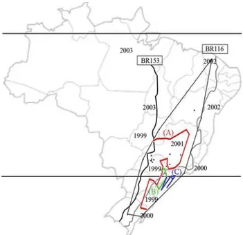
Specimens ofZ. indianuswere collected from 2004 to 2007, in 22 localities of Brazil (Table 1), 13 in the state of São Paulo (SP), three in Minas Gerais (MG), two in Rio Grande do Sul (RS), and one each in Santa Catarina (SC), Rio de Janeiro (RJ), Bahia (BA), and Brasilia (DF). Indi-viduals were collected with traps containing enticing baits made up of banana and biological yeast, as described by Galegoet al.(2006). Figure 1 shows the scatterplot of the locations of the populations sampled, with the enclosing convex polygon overlaid by the map of Brazil. Analysis was restricted to collections with more than 10 individuals. Collected individuals were maintained in mass culture with banana-agar medium. A random sample of 20 flies (10 males and 10 females, all 7 days old) of individuals emerg-ing from eggs ovoposited by females from nature, were used for esterase detection.
Polyacrylamide gel electrophoresis and esterase detection
Each individual fly was macerated in 15mL of Tris-HCl 0.1 M, pH 8.8 (CR Ceron, MSc Dissertation, Uni-versidade de São Paulo, 1988), whereupon the homogenate was applied to a 10% polyacrylamide gel. Electrophoresis was carried out in a Tris-glycine buffer pH 8.8 at 200 V for 3 h. A random sample of 20 individuals (10 males and 10 females) from each population was used. In the case of the EST2 system, which is restricted to males (Galegoet al., 2006), only 10 individuals were analyzed. Detection of the esterases (EST) was undertaken as suggested by Galegoet al. (2006). After detection, the gels were stored as de-scribed by Ceronet al.(1992).
Data analysis
Alloenzyme data were analyzed using the computer software programmes TFPGA version 1.3 (Miller, 1997), Genetic Analyses in Excel (GenAlEx) version 6 (Peakall and Smouse, 2006), and Alleles in Space -AIS- (Miller, 2005). Allele and genotype polymorphic-locus frequen-cies, observed (HO) and expected (HE) heterozygosity, and Hardy-Weinberg equilibrium, were all estimated by TFPGA. The estimation of genetic distances (Nei, 1972) and FSTanalysis were undertaken with GenAlEx. AIS anal-ysis of Landscape Shape Interpolation (LSI) and the Mon-monier Maximum Difference Algorithm (MMDA), was performed to evaluate inter-individual patterns of genetic and geographical variation. The calculated surface for LSI was based on the midpoints of edges derived from Delau-nay triangulation (Watson, 1992; Brounset al., 2003), and the heights on “pseudoslopes” from the genetic and geo-graphical distance matrix (Miller, 2005). The LSI approach visualizes the graphical representation of the pattern of ge-netic distance across the whole landscape, and is a way of producing a 3-dimensional surface plot where the X and Y axes correspond to geographical locations, whereas surface heights (Z-axes) represent genetic distances. Basically, the figure contains an inferred graphical representation of pat-terns of diversity across the sampled landscape that (ide-ally) contains peaks in areas where there are large genetic distances. The initial construction is Delaunay triangula-tion (Watson, 1992; Brounset al., 2003) based on connec-tivity networks of sampling areas and assigning genetic distances, whereupon interpolation procedure (a = 1, grid size = 50 x 50, raw Nei, 1972, genetic distance between points) can be applied.
Furthermore, the building of putative genetic barriers across landscapes, as determined by MMDA, is found in the connectivity network of all the sampled locations used in studies that are generated in three steps by Delaunay tri-angulation (Watson, 1992; Brounset al., 2003). The first step is to identify the greatest genetic distance between any 2 locations joined in the connectivity network, thereby forming the initial barrier segment. Secondly, the initial
Figure 1- Delaunay triangulation (fine black line) and genetic boundaries in heavy red (A), green (B) and blue (C) lines obtained with the Mon-monier maximum difference algorithm. Note that (A) separates the coastal populations, the localities in south-eastern São Paulo state and northern populations from the rest, (B) encompasses the two south-eastern São Paulo populations, thereby isolating them, and (C) isolates coastal popula-tions of the Brazilian south-east and south. The irregular parallel lines across the map of Brazil indicate the BR153 (black line) and BR 116 (gray line) freeways. The numbers indicate the years whenZaprionus indianus
barrier is followed in one direction until encountering ei-ther an external edge of the connectivity network or an in-ternal segment previously defined as a barrier segment. In essence, for each extension of the barrier, the movement is in the direction of the greatest genetic distance between lo-cations. Finally, the initial barrier identified in Step 1 is fol-lowed in the opposite direction to that taken in Step 2, until, once again, encountering either an external edge of the con-nectivity network or an internal segment previously de-fined as a barrier segment.
Results
The analysis of Est2 allele frequency distribution in Brazilian populations ofZ. indianus(Table 1) shows
fixa-tion of the alleles Est2Sin 8 of the 22 populations studied, and Est2Fin 3. Est2Sfrequency was the lowest in Alfenas (0.09), and that of Est2Fin Onda Verde and Rio de Janeiro (0.08). The frequency of locus Est3 alleles (Table 1) varied considerably according to geographic location, the least frequent being Est33. Est31frequency varied from 0 (Ilha-bela) to 0.94 (Santa Maria), Est34from 0.05 (Rio Claro and Porto Alegre) to 0.89 (Ilhabela), and Est33from 0 (in sev-eral localities) to 0.30 (Onda Verde). The frequency of Est32, although not detected in Santa Maria, Onda Verde and Ilhabela, was the highest in Brasília (0.69).
The average observed (HO) and expected (HE) was greater in Est3 than in Est2 (Table 2). Est3 HOranged from 0 (Ilhabela) to 0.80 (Onda Verde) and HEfrom 0.20
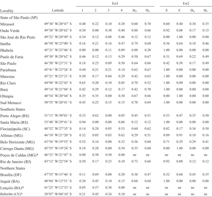
(Ilha-Table 1- Geographical coordinates of theZaprionus indianuspopulations sampled and allele frequencies of Est3 and Est2 esterase loci. 1: Est31; 2: Est32;
3: Est33; 4: Est34; S: Est2S; F: Est2F; HO: observed heterozygosity; HE: expected heterozygosity; ne: not evaluated. *Mattos-Machadoet al. (2005).
Est3 Est2
Locality Latitude 1 2 3 4 HO HE S F HO HE
State of São Paulo (SP)
Mirassol 49°30’ W/20°47’ S 0.40 0.22 0.10 0.28 0.60 0.70 0.60 0.40 0.30 0.35
Onda Verde 49°30’ W/20°62’ S 0.30 0.00 0.30 0.40 0.80 0.66 0.92 0.08 0.17 0.15
São José do Rio Preto 49°22’ W/20°49’ S 0.34 0.12 0.08 0.46 0.12 0.12 0.00 1.00 0.00 0.00
Itatiba 46°50’ W/23°00’ S 0.16 0.21 0.16 0.47 0.79 0.68 0.36 0.64 0.18 0.46
Ilhabela 45°21’ W/23°46’ S 0.00 0.00 0.11 0.89 0.00 0.20 1.00 0.00 0.00 0.00
Paulo de Faria 49°30’ W/20°62’ S 0.46 0.12 0.13 0.29 0.50 0.67 0.31 0.69 0.22 0.49
São Paulo 46°50’ W/23°31’ S 0.18 0.23 0.09 0.50 0.64 0.66 0.42 0.58 0.17 0.49
Paraibuna 45°41’ W/23°26’ S 0.44 0.21 0.21 0.14 0.62 0.67 1.00 0.00 0.00 0.00
Maresias 45°21’ W/23°21’ S 0.50 0.17 0.04 0.29 0.42 0.63 1.00 0.00 0.00 0.00
Rio Claro 44°08’ W/22°43’ S 0.65 0.20 0.10 0.05 0.70 0.52 1.00 0.00 0.00 0.00
Ibirá 49°14’ W/21°04’ S 0.42 0.29 0.12 0.17 0.42 0.70 1.00 0.00 0.00 0.00
Olímpia 48°54’ W/20°44’ S 0.35 0.35 0.00 0.30 0.67 0.66 0.00 1.00 0.00 0.00
Sud Menucci 50°55’ W/20°41’ S 0.45 0.25 0.15 0.15 0.70 0.69 1.00 0.00 0.00 0.00
Southern States
Porto Alegre (RS) 51°13’ W/30°01’ S 0.33 0.62 0.00 0.05 0.45 0.51 0.53 0.47 0.35 0.50
Santa Maria (RS) 53°48’ W/29°41’ S 0.94 0.00 0.00 0.06 0.12 0.12 1.00 0.00 0.00 0.00
Florianópolis (SC) 48°32’ W/27°35’ S 0.14 0.28 0.05 0.53 0.60 0.62 0.82 0.17 0.36 0.30
Alfenas (MG) 46°10’ W/21°20’ S 0.32 0.03 0.03 0.62 0.29 0.51 0.09 0.91 0.18 0.16
Belo Horizonte (MG) 43°56’ W/19°55’ S 0.52 0.16 0.00 0.32 0.56 0.60 0.71 0.29 0.29 0.41
Córrego Danta (MG) 45°55’ W/19°24’ S 0.18 0.28 0.00 0.54 0.53 0.60 0.00 1.00 0.00 0.00
Poços de Caldas (MG)* 46°33’ W/21°47’ S 0.00 0.50 0.50 0.00 ne ne ne ne ne ne
Rio de Janeiro (RJ) 43°12’ W/22°54’ S 0.50 0.17 0.23 0.10 0.73 0.66 0.92 0.08 0.12 0.12
Northern States
Brasília (DF) 47°55’ W/15°46’ S 0.11 0.69 0.00 0.20 0.38 0.47 0.32 0.68 0.45 0.35
Jequié (BA) 40°04’ W/13°51’ S 0.30 0.45 0.10 0.15 0.60 0.68 1.00 0.00 0.00 0.00
Lençóis (BA)* 41°23’ W/12°33’ S 0.05 0.57 0.38 0.00 ne ne ne ne ne ne
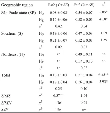
bela) to 0.70 (Mirassol and Ibirá). The average Est3 HOin populations from São Paulo state (0.54± 0.07), and the southern (0.47±0.08) and northern (0.49±0.11) states did not differ significantly (X2= 0.10). On the other hand, Est2 HOranged from 0 (11 populations) to 0.45 (Brasilia), and HEfrom 0 (11 populations) and 0.50 (Porto Alegre). The average Est2 HO in populations from São Paulo state (0.08±0.03) and southern regions (0.19±0.06) were not significantly different. Almost all the populations, except those from Ibirá and Maresias, were estimated to be under Hardy-Weinberg equilibrium, with p < 0.05.
Pairwise genetic distance (Nei 1972) and FST(Weir and Cockerham, 1984) indices differed significantly from zero in several populations (Table S1). About 91% of the pairwise FSTvalues were significantly different from zero. The overall FST value was 0.414 (p < 0.001), and the pairwise estimates of FSTranged from 0.003 (Sud Menucci versus Paraibuna) to 1.000 (Santa Maria versus Poços de Caldas).
Genetic boundaries depicted in Est2 and Est3 data are shown in Figure 1. The first boundary (A) separated the coastal populations (Rio de Janeiro, Maresias, Ilhabela and Florianópolis), the localities in south-eastern São Paulo state (Paraibuna, Itatiba, São Paulo and Rio Claro) and northern populations (Brasília, Jequié, Lençóis and Bebe-ribe), from the rest. The second boundary (B) enclosed Itatiba and São Paulo, thereby isolating both populations. The last (C), isolated Florianópolis, Maresias and Ilhabela and coincided with the geological formation composed of
the Serra do Mar Range. Genetic Landscape Shape Interpo-lation analysis (Figure 2) generated peaks indicating the greatest genetic distances in populations from São Paulo, Itatiba and other localities of south-eastern São Paulo state, decreasing from there in direction to the north and south of Brazil.
Discussion
Originally from tropical Africa, historical records show that Z. indianus arrived in Brazil in 1998 (Vilela, 1999), and quickly spread throughout São Paulo (Vilelaet al., 2000), Rio de Janeiro (Loh and Bitner-Mathé, 2005), and the southern (Toni et al., 2001; Castro and Valente 2001) and midwestern (Tidonet al., 2003) states. The re-maining Brazilian regions were thereafter rapidly colo-nized (Santoset al., 2003; Katoet al., 2004; Mataet al., 2004; Mattos-Machadoet al., 2005), 5 years after the first records in Para, one of the most northerly states in Brazil (Santoset al., 2003).
The polymorphism displayed by both alloenzyme markers demonstrated a significant geographical genetic structure among the 22 Brazilian populations ofZ. indianus sampled in this study, as shown by the FSTand Nei (1972) genetic distance values. The Est3 HOvalues of the Brazilian populations ofZ. indianus(0.54) were almost the same as the three esterase HO of Indian population loci, each of which harboring 5 alleles,i.e., 0.54 and 0.56 (Parkashet al., 1994) and 0.58 (Parkash and Yadav, 1993), respectively. However, the Est2 HOvalues from Brazilian populations (0.08) were smaller than an esterase locus with two alleles in Indian populations, viz., 0.17 (Parkash and Yadav, 1993) and 0.33 (Parkashet al., 1994). These differences could be attributed to genetic drift (sampling errors) or the founder effect.
Table 2- Means (X) and standard-errors (SE) of observed (HO) and
ex-pected (HE) heterozygosity in Brazilian populations ofZaprionus indianus
and chi-squared comparison (x2). ne: not evaluated.
Geographic region Est2 (X±SE) Est3 (X±SE) x2
São Paulo state (SP) HO 0.08±0.03 0.54±0.07 5.05*
HE 0.15±0.06 0.58±0.05 4.18*
x2 0.42 0.04
Southern (S) HO 0.19±0.06 0.47±0.08 1.19
HE 0.21±0.07 0.52±0.07 1.25
x2 0.02 0.03
Northeast (N) HO ne 0.49±0.11 ne
HE ne 0.57±0.10 ne
x2 ne 0.02
Total HO 0.13±0.03 0.51±0.04 6.35**
HE 0.17±0.04 0.56±0.04 5.93*
x2 0.25 0.10
SPXS x2 6.37** 1.04
SPXN x2 Ne 0.51
SXN x2 Ne ne
*p <0.05; **p <0.01; ***p <0.001.
Allele frequencies were employed in the relatively promising, but little used, methodologies of spatial interpo-lation (Storferet al., 2007) and the Monmonier algorithm. These approaches could be especially useful in the case of continuously distributed species, by representing allele fre-quency across a landscape surface, and identifying putative genetic barriers. Normally, mitochondrial DNA markers have been used in these analyses (Dupanloupet al., 2002). By using mtDNA HVRI polymorphism, it was thus possi-ble to infer the action of a past specific barrier hindering gene flow between Italian and Balkanic populations of the European roe deer. Moreover, Manni et al. (2004) sug-gested that the Monmonier algorithm could also be applied in the identification of barriers by using geographical pat-terns of genetic, morphological and linguistic variation.
The application of these approaches to our data facili-tated depicting the graphic pattern of the ratio between ge-netic and geographic distances (pseudoslope) throughout the sampled regions, with the surface edges corresponding to the highest ratios. All the edges were located in south-eastern Brazil, specifically São Paulo state, thereby indicat-ing the higher genetic structurindicat-ing of these populations, possibly due to both early origin and low gene flow. Histor-ical data reinforce the idea of the earlier arrival of Z. indianusin São Paulo state, whereas the 2 highest peaks in the graphical surface, isolated by A and B putative barriers, as inferred by MMDA analysis, suggest population isola-tion. Based on these clues, analysis of genetic data rein-forces the hypothesis that São Paulo state was the center from whichZ. indianusspread throughout Brazil. On the other hand, the northern and southern populations pre-sented the lowest ratios between genetic and geographic distances, as shown by depressions in the graph-surface. This landscape indicated lower genetic structuring, proba-bly due to a later invasion.This scenario agrees with the above-cited historical records.
By identifying 3 boundaries for gene flow through MMDA analysis, a putative scenario of the spread ofZ. indianusin Brazil can be visualized (Figure 1). Boundary A separates the coastal populations from the remainder, boundary B isolates the towns of São Paulo and Itatiba, both located very close to Valinhos, whereZ. indianuswas first observed, whereas boundary C corresponds to a natu-ral geological barrier, the Serra do Mar, a 1500 km long mountain range extending from Espírito Santo to Santa Catarina states. These boundaries separate two of the main highways in Brazil, the BR153 and BR116. The first is an important route for commercial interchange with inland Brazil (Confederação Nacional de Transportes a), whereas the second is coastal (Confederação Nacional de Trans-portes b). A similar manner of diffusion, due to the fruit trade, may have occurred in the Palearctic region (Yassinet al., 2009). However, in the Americas the spread was ex-tremely fast (about six years, from São Paulo to Florida), in contrast to the Palearctic region, where it took more than 40
years forZ. indianus to spread from India to Egypt. The great difference in the pace of spread between Brazil/USA and India/Egypt can be attributed to the more developed freeway networks in Brazil than in the Palearctic region.
These findings suggest that the spreading of Z. indianusoccurred from São Paulo, the state where com-mercial highway traffic is the heaviest, to the north and south of Brazil by way of both the BR153 and the BR116 highways. The landscape genetics approach hereby applied for characterizing the genetic structure of populations from an initial colonizer species soon after its introduction, as well as its relevance in offering the possibility of determin-ing the source of invasion, and demographic parameters of the species, also offers a unique opportunity for accompa-nying the evolutionary dynamics of the invader species over time.
Acknowledgments
This work was supported by FAPESP (04/05235-7) and CNPq.
References
Ananina G, Rohde C, David JR, Valente VL and Klaczko LB (2006) Inversion polymorphism and a new polytene chro-mosome map ofZaprionus indianusGupta (1970) (Diptera, Drosophilidae). Genetica 131:117-125.
Arnaud JF (2003) Metapopulation genetic structure and migration pathways in the land snailHeliz aspersa: Influence of land-scape heterogeneity. Landland-scape Ecol 18:333-346.
Brouns G, De Wulf A and Constales D (2003) Delaunay triangu-lation algorithms useful for multibeam echosounding. J Surv Eng 129:79-84.
Castro FL and Valente VLS (2001)Zaprionus indianusinvading communities in the southern Brazilian city of Porto Alegre. Drosophila Inf Serv 84:15-17.
Ceron CR, Santos JR and Campos Bicudo HEM (1992) The use of gelatin to dry cellophane wound slab gels in an embroider-ing hoop. Rev Bras Genet 15:201-203.
David JR, Araripe LO, Bitner-Mathe BC, Capy P, Goñi B, Klaczo LB, Legout H, Martins MB, Vouidibio J, Yassin A,et al. (2006a) Sexual dimorphism of body size and sternopleural britle number: A comparison of geographic population of an invasive cosmopolitan drosophilid. Genetica 128:109-122. David JR, Araripe LO, Bitner-Mathe BC, Capy P, Goñi B, Klaczo
LB, Legout H, Martins MB, Vouidibio J, Yassin A,et al. (2006b) Quantitative trait analyses and geographic variabil-ity of natural populations ofZaprionus indianus, a recent in-vader in Brazil. Heredity 96 53-62.
Dupanloup I, Schneider S and Excoffier L (2002) A simulated an-nealing approach to define the genetic structure of popula-tions. Mol Ecol 11:2571-2581.
Galego LGC, Ceron CR and Carareto CMA (2006) Characteriza-tion of esterases in a Brazilian populaCharacteriza-tion of Zaprionus Indianus(Diptera, Drosophilidae). Genetica 126:89-99. Goñi B, Fresia P, Calviño M, Ferreiro MJ, Valente VLS and Basso
da Silva L (2001) First record ofZaprionus indianusGupta, 1970 (Diptera, Drosophilidae) in southern localities of Uru-guay, South America. Drosophila Inf Serv 84:61-65. Goñi B, Martinez ME, Techera G and Fresia P (2002). Increased
frequencies of Zaprionus indianusGupta, 1970 (Diptera, Drosophilidae) in Uruguay. Drosophila Inf Serv 85:75-80. Guillot G, Estoup A, Mortier F and Cosson JF (2005) A spatial
statistical model for landscape genetics. Genetics 170:1261-1280.
Hirao AS and Kudo G (2004) Landscape genetics of alpine-snowbed plants: Comparisons along geographic and snowmelt gradients. Heredity 93:290-298.
Hitchings SP and Beebee TJC (1997) Genetic substructuring as a result of barriers to gene flow in urban Rana temporaria (common frog) populations: Implications for biodiversity conservation. Heredity 79:117-127.
Holderegger R and Wagner HH (2006) A brief guide to landscape genetics. Landscape Ecol 21:793-796.
Isaaks EH and Srivastava RM (1989) An Introduction to Applied Geostatistics. Oxford University Press, New York, 592 pp. Jacquemyn H (2004) Genetic structure of the forest herbPrimula
elatiorin a changing landscape. Mol Ecol 13:211-219. Kato CM, Foureaux LV, César RA and Torres MP (2004)
Ocor-rência de Zaprionus indianus Gupta, 1970 (Diptera, Drosophilidae) no estado de Minas Gerais. Ciênc Agrotec 28:454-455 (Abstract in English).
Liepelt S, Bialozyt R and Ziegenhage B (2002) Wind-dispersed pollen mediates postglacial gene flow among refugia. Proc Natl Acad Sci USA 99:14590-14594.
Linde K, Steck GJ, Hibbard K, Birdsley JS, Alonso LM and Houle D (2006) First records of Zaprionus indianus (Diptera, Drosophilidae), a pests species on commercial fruits from Panama and the United States of America. Fla Entomol 89:402-403.
Loh R and Bitner-Mathe BC (2005) Variability of wing size and shape in three populations of a recent Brazilian invader Zaprionus indianus(Diptera, Drosophilidae) from different habitats. Genetica 125:271-281.
Manel S, Schwartz ML, Luikart G and Taberlet P (2003) Land-scape genetics: Combining landLand-scape ecology and popula-tion genetics. Trends Ecol Evol 18:189-197.
Manni F, Guerard E and Heyer E (2004) Geographic patterns of (genetic, morphologic, linguistic) variation: How barriers can be detected by using Monmonier’s algorithm. Hum Biol 76:173-190.
Mattos-Machado T, Solé-Cava AM, David JR and Bitner-Mathé BC (2005) Allozyme variability in an invasive drosophilid, Zaprionus indianus(Diptera, Drosophilidae): Comparison of a recently introduced Brazilian population with Old World populations. Ann Soc Entomol Fr 41:7-13.
Miller MP (1997) Tool for population genetic analyses – TFPGA -1.3: A Windows program for the analysis of allozyme and molecular population genetic data. Computer software dis-tributed by author.
Miller MP (2005) Alleles in space (AIS): Computer software for the joint analysis of interindividual spatial and genetic infor-mation. J Hered 96:722-724.
Michels E, Cottenie K, Neys L, DeGalas K, Coppin P and DeMe-ester L (2001) Geographical and genetic distances among zooplankton populations in a set of interconnected ponds: A plea for using GIS modeling of the effective geographical distance. Mol Ecol 10:1929-1938.
Monmonier MS (1973) Maximum-difference barriers: An alter-native numerical regionalization method. Geogr Anal 5:245-261.
Nei M (1972) Genetic distance between populations. Am Nat 106:283-292.
Parkash R and Yadav JP (1993) Geographical clinal variation at seven esterase encoding loci in Indian populations of Zaprionus indianus. Hereditas 119:161-173.
Parkash R, Yadav JP and Vashist M (1994) Electrophoretic and cryptic genic variability in natural populations ofZaprionus indianus. Proc Indian Nat Sci Acad B60:75-82.
Peakall R and Smouse PE (2006) GENALEX 6: Genetic analysis in Excel. Population genetic software for teaching and re-search. Mol Ecol Notes 6:288-295.
Pfenninger M (2002) Relationship between microspatial popula-tion genetric structure and habitat heterogeneity inPomatias elegans (O.F. Muller 1774) (Caenogastropoda, Pomatia-sidae). Biol J Linn Soc Lond 76:565-575.
Poissant J, Knight TW and Ferguson MM (2005). Nonequilibrium conditions following landscape rearrangement: The relative contribution of past and current hydrological landscapes on the genetic structure of a stream-dwelling fish. Mol Ecol 14:1321-1331.
Santos JF, Rieger TT, Campos SRC, Nascimento ACC, Félix PT, Silva SVO and Freitas FMR (2003) Colonization of North-east Region of Brazil by the drosophilid flies Drosophila malerkotlianaandZaprionus indianusa new potential insect pest for Brazilian fruitculture. Drosophila Inf Serv 86:92-95. Storfer A, Murphy MA, Evans JS, Goldberg CS, Robinson S, Spear SF, Dezzani R, Delmelle E, Vierling L and Waits LP (2007) Putting the “landscape” in the landscape genetics. Heredity 98:128-142.
Tidon R, Leite DF and Leão BFD (2003) Impact of the coloniza-tion ofZaprionus indianus(Diptera, Drosophilidae) in dif-ferent ecosystems of the neotropical region: 2 years after the invasion. Biol Conserv 112:299-305.
Toni DC, Hofmann PRP and Valente VLS (2001) First register of Zaprionus indianus(Diptera, Drosophilidae) in the state of Santa Catarina, Brazil. Biotemas 14:71-85.
Vilela CR (1999) IsZaprionus indianusGupta, 1970 (Diptera, Drosophilidae) currently colonizing the Neotropical region? Drosophila Inf Serv 82:37-39.
Vilela CR, Teixeira EP and Stein CP (2000) Mosca-africana-do-figo, Zaprionus indianus (Diptera, Drosophilidae). In: Vilela E, Zucchi RA and Cantor F (eds) Histórico e Impacto das Pragas Introduzidas no Brasil. Editora Holos, São Paulo, pp 48-52.
Watson DF (1992) Contouring: A guide to the analysis and dis-play of spatial data. Pergamon Press, New York, 321 pp. Weir BS and Cockerham CC (1984) Estimating F-statistics for the
analysis of population structure. Evolution 38:13.
Internet Resources
Confederação Nacional de Transportes (CNT)a, http://www. cnt.org.br/informacoes/pesquisas/rodoviaria/2007/arquivos /pdf/ligacao057.pdf (March 20, 2010).
Confederação Nacional de Transportes (CNT)b, http:// www.cnt.org.br/informacoes/pesquisas/rodoviaria/2007/ar quivos/pdf/ligacao048.pdf (March 20, 2010).
Mata RM, Kanegae MF and Tidon R (2004) Diagnóstico am-biental do Parque estadual do Jalapão mediante a análise da fauna de Drosofilídeos (Insecta, Díptera). XXV Congresso Brasileiro de Zoologia, Abstract, http://www.zoologia. bio.br/congressos/CBZ/resumos/XXVCBZcompleto-111. html (April 5, 2009).
Supplementary Material
The following online material is available for this ar-ticle:
Table S1 - Pairwise values of FSTand genetic distance between the Brazilian populations ofZaprionus indianus.
This material is available as part of the online article from http://www.scielo.br/gmb.
Associate Editor: Fábio de Melo Sene
(Florianópolis), PA (Porto Alegre) and SM (Santa Maria); andNorth and Mideast states:BR (Brasília), JE (Jequié), LE*(Lençóis) and BE*(Beberibe). *Machadoet al.2005.
IB IL IT MA MI OL OV PF PR RC SJ SU SP AL BH CD RJ BR FL PA SM JE LE* BE* PC*
IB ***** 0.226 0.460 0.015 0.099 0.767 0.086 0.458 0.013 0.039 0.797 0.006 0.425 0.727 0.105 0.798 0.033 0.511 0.100 0.232 0.117 0.013 0.704 0.581 0.752
IL 0.296 ***** 0.354 0.195 0.267 0.827 0.111 0.527 0.281 0.376 0.734 0.274 0.388 0.559 0.266 0.716 0.319 0.664 0.070 0.560 0.439 0.263 0.963 0.851 0.948
IT 0.272 0.299 ***** 0.452 0.181 0.160 0.336 0.075 0.498 0.562 0.116 0.493 0.011 0.085 0.260 0.107 0.449 0.182 0.256 0.282 0.619 0.473 0.713 0.605 0.718
MA 0.015 0.285 0.277 ***** 0.093 0.753 0.076 0.428 0.031 0.038 0.762 0.019 0.411 0.667 0.067 0.780 0.045 0.570 0.101 0.287 0.078 0.053 0.830 0.654 0.879
MI 0.108 0.233 0.068 0.110 ***** 0.382 0.117 0.148 0.115 0.128 0.394 0.105 0.142 0.352 0.023 0.411 0.087 0.287 0.111 0.130 0.176 0.126 0.703 0.530 0.749
OL 0.504 0.634 0.133 0.507 0.245 ***** 0.741 0.089 0.795 0.770 0.028 0.777 0.120 0.089 0.444 0.026 0.706 0.162 0.630 0.318 0.767 0.772 0.734 0.597 0.801
OV 0.060 0.118 0.179 0.059 0.068 0.449 ***** 0.385 0.080 0.147 0.677 0.090 0.345 0.574 0.128 0.720 0.083 0.608 0.099 0.399 0.206 0.133 0.830 0.710 0.787
PF 0.278 0.386 0.024 0.273 0.064 0.099 0.203 ***** 0.466 0.456 0.075 0.457 0.040 0.081 0.183 0.115 0.385 0.227 0.378 0.249 0.449 0.500 0.788 0.600 0.813
PR 0.012 0.344 0.286 0.031 0.115 0.519 0.058 0.282 ***** 0.023 0.817 0.003 0.464 0.765 0.122 0.846 0.009 0.569 0.160 0.267 0.094 0.035 0.704 0.590 0.722
RC 0.046 0.483 0.334 0.048 0.133 0.538 0.099 0.301 0.030 ***** 0.813 0.017 0.500 0.770 0.102 0.856 0.021 0.605 0.233 0.272 0.030 0.075 0.779 0.612 0.827
SJ 0.517 0.580 0.116 0.512 0.249 0.027 0.422 0.093 0.529 0.559 ***** 0.807 0.099 0.029 0.446 0.022 0.725 0.255 0.615 0.433 0.792 0.826 0.843 0.696 0.862
SU 0.006 0.343 0.286 0.020 0.112 0.513 0.063 0.280 0.003 0.023 0.526 ***** 0.452 0.749 0.105 0.828 0.014 0.551 0.146 0.249 0.083 0.028 0.718 0.588 0.754
SP 0.258 0.315 0.003 0.260 0.056 0.118 0.180 0.013 0.273 0.311 0.110 0.270 ***** 0.077 0.205 0.093 0.410 0.154 0.256 0.223 0.542 0.441 0.719 0.577 0.752
AL 0.464 0.462 0.067 0.447 0.199 0.070 0.351 0.060 0.483 0.521 0.038 0.478 0.064 ***** 0.378 0.047 0.688 0.315 0.498 0.477 0.738 0.773 0.952 0.769 0.969
BH 0.103 0.240 0.107 0.090 0.010 0.283 0.069 0.086 0.111 0.115 0.284 0.104 0.088 0.226 ***** 0.482 0.094 0.408 0.140 0.210 0.104 0.159 0.853 0.621 0.912
CD 0.525 0.579 0.115 0.528 0.260 0.027 0.447 0.112 0.548 0.587 0.022 0.543 0.110 0.050 0.305 ***** 0.772 0.172 0.572 0.382 0.867 0.800 0.768 0.650 0.819
RJ 0.038 0.212 0.217 0.045 0.058 0.436 0.034 0.203 0.027 0.038 0.444 0.030 0.203 0.402 0.056 0.469 ***** 0.539 0.188 0.247 0.076 0.064 0.711 0.579 0.722
BR 0.320 0.489 0.072 0.354 0.124 0.134 0.302 0.085 0.345 0.392 0.172 0.340 0.062 0.166 0.185 0.142 0.281 ***** 0.391 0.095 0.723 0.446 0.423 0.397 0.532
FL 0.077 0.106 0.137 0.082 0.056 0.394 0.044 0.188 0.101 0.148 0.386 0.097 0.136 0.308 0.067 0.371 0.077 0.214 ***** 0.265 0.328 0.104 0.739 0.628 0.786
PA 0.173 0.382 0.102 0.203 0.048 0.221 0.182 0.097 0.189 0.213 0.266 0.183 0.083 0.249 0.086 0.253 0.134 0.052 0.130 ***** 0.377 0.188 0.439 0.360 0.559
SM 0.211 0.748 0.434 0.170 0.209 0.624 0.182 0.368 0.185 0.097 0.637 0.171 0.402 0.610 0.167 0.687 0.109 0.533 0.254 0.343 ***** 0.186 0.951 0.717 1.000
JE 0.013 0.333 0.279 0.052 0.120 0.510 0.079 0.296 0.032 0.086 0.534 0.027 0.266 0.488 0.127 0.530 0.052 0.293 0.080 0.156 0.295 ***** 0.601 0.523 0.662
LE 0.557 0.735 0.448 0.601 0.439 0.572 0.541 0.467 0.560 0.617 0.597 0.566 0.445 0.601 0.499 0.588 0.516 0.418 0.514 0.403 0.757 0.533 ***** 0.077 0.035
BE 0.514 0.672 0.408 0.540 0.390 0.523 0.494 0.412 0.518 0.554 0.543 0.519 0.400 0.535 0.432 0.541 0.470 0.406 0.470 0.377 0.667 0.504 0.516 ***** 0.148