Full Terms & Conditions of access and use can be found at
http://www.tandfonline.com/action/journalInformation?journalCode=ujoa20
Download by: [Universidade Nova de Lisboa] Date: 21 November 2017, At: 09:17
Journal of Advertising
ISSN: 0091-3367 (Print) 1557-7805 (Online) Journal homepage: http://www.tandfonline.com/loi/ujoa20
Bridging Design and Behavioral Research With
Variance-Based Structural Equation Modeling
Jörg Henseler
To cite this article: Jörg Henseler (2017) Bridging Design and Behavioral Research With Variance-Based Structural Equation Modeling, Journal of Advertising, 46:1, 178-192, DOI: 10.1080/00913367.2017.1281780
To link to this article: https://doi.org/10.1080/00913367.2017.1281780
© 2017 The Author(s). Published with license by Taylor & Francis© Jörg Henseler
Published online: 07 Feb 2017.
Submit your article to this journal
Article views: 2141
View related articles
View Crossmark data
Bridging Design and Behavioral Research With
Variance-Based Structural Equation Modeling
J
€
org Henseler
University of Twente, Enschede, the Netherlands, and Universidade Nova de Lisboa, Lisboa, Portugal
Advertising research is a scientific discipline that studies artifacts (e.g., various forms of marketing communication) as well as natural phenomena (e.g., consumer behavior). Empirical advertising research therefore requires methods that can model design constructs as well as behavioral constructs, which typically require different measurement models. This article presents variance-based structural equation modeling (SEM) as a family of techniques that can handle different types of measurement models: composites, common factors, and causal–formative measurement. It explains the differences between these types of measurement models and clears up possible ambiguity regarding formative endogenous constructs. The article proposes confirmatory composite analysis to assess the nomological validity of composites, confirmatory factor analysis (CFA) and the heterotrait-monotrait ratio of correlations (HTMT) to assess the construct validity of common factors, and the multiple indicator, multiple causes (MIMIC) model to assess the external validity of causal–formative measurement.
Advertising research is a relatively young academic disci-pline that combines design research and behavioral research. On one hand, advertising research covers “knowledge unique to advertising as an institution and professional practice” (Reid 2014, p. 410). It investigates what is understood as advertising in the widest sense, including the whole range of marketing communication and branding. In this sense, adver-tising forms a class of marketing instruments that can be viewed as artifacts designed by humans. The term artifact
should be understood broadly, but not as a statistical or meth-odological artifact despite the methmeth-odological character of this
article.1Advertising research with this focus is a “science of the artificial” (Simon 1969) and thus a design science, aiming to generate a body of knowledge on how to create, improve, orchestrate, and manage specific types of marketing instru-ments. On the other hand, advertising research is predomi-nantly regarded as a behavioral science (Carlson 2015), aiming to explain advertising effects and the social aspects of advertising (Reid 2014). Advertising research with this focus sheds light on consumers and can be viewed as a particular type of consumer research and applied psychology. This dual focus poses challenges for its theories as well as the empirical methods to create and validate them.
Empirical advertising research on relationships between behavioral constructs and design constructs needs analytical tools that can cope with the different requirements of behav-ioral and design sciences. Behavbehav-ioral constructs are often latent variables that can be understood as ontological entities, such as attributes or attitudes of consumers. This way of theo-retical reasoning rests on the assumption that theotheo-retical con-structs of interest exist in nature, irrespective of scientific investigation. In contrast, constructs of design research (arti-facts) can be conceived as products of theoretical thinking. Thinking about constructs as artifacts has its roots in construc-tivist epistemology. Constructs in this sense can be understood as constructions that are theoretically justified. The epistemo-logical distinction between the ontoepistemo-logical and the constructiv-ist nature of constructs has important design implications. The correspondence rule that links the empirical indicators to the theoretical construct, as conceptually represented in what is referred to as the measurement model, depends on the nature of the construct. Whereas behavioral constructs are typically modeled as common factors, design constructs can be modeled as composites. Modeling design constructs as composites pays tribute to the fact that all artifacts or abstractions thereof con-sist of more elementary components (Nelson and Stolterman 2003).
Against this background, this article illustrates the use of variance-based structural equation modeling (SEM) as an ana-lytical tool for empirical advertising research at the interface of design and behavioral research. Unlike covariance-based SEM, variance-based SEM can estimate common factors and Address correspondence to J€org Henseler, Department of Design,
Production, and Management, University of Twente, Drienerlolaan 5, 7522 NB, Enschede, the Netherlands. E-mail: [email protected]
J€org Henseler (PhD, University of Kaiserslautern) is Chair of Product-Market Relations, and Head of the Department of Design, Production, and Management, Faculty of Engineering Technology, University of Twente, Enschede, the Netherlands and Visiting Profes-sor, Nova Information Management School, Universidade Nova de Lisboa, Lisboa, Portugal.
This is an Open Access article distributed under the terms of the Creative Commons Attribution License (http://creativecommons.org/ licenses/by/4.0/), which permits unrestricted use, distribution, and reproduction in any medium, provided the original work is properly cited.
178
ISSN: 0091-3367 print / 1557-7805 online DOI: 10.1080/00913367.2017.1281780
composites, which makes it suitable for behavioral constructs as well as design constructs. The remainder of this article is organized as follows: It begins by explaining the nature of var-iance-based SEM and how to specify structural equation mod-els containing composites as well as common factors. This includes the different specifications of measurement models (composite, reflective, and causal–formative) as well as struc-tural models. Next, it describes how to conduct model tests, how to assess and report estimates of variance-based SEM, and the use of the bootstrap for inference statistics. Finally, it discusses extensions of variance-based SEM and provides sug-gestions for further research.
VARIANCE-BASED STRUCTURAL EQUATION MODELING
As in several other scientific disciplines, theoretical con-structs are the building blocks of advertising theories. A theo-retical construct is “a conceptual term used to describe a phenomenon of theoretical interest” (Edwards and Bagozzi 2000, pp. 156–57). Generally speaking, most theoretical constructs “can only be measured through observable meas-ures or indicators that vary in their degree of observational meaningfulness and validity. No single indicator can capture the full theoretical meaning of the underlying construct and hence, multiple indicators are necessary” (Steenkamp and Baumgartner 2000, p. 196).
Common theoretical constructs in advertising research are, for instance, attitude toward the brand, ad liking, ad awareness, advertising practices, media mix, advertising budget, and advertising content. Whereas some theoretical constructs of advertising research refer to consumer attributes, others refer to human-made objects (artifacts) that are typically created by managers, staff, or other agents of firms.
To empirically investigate relationships between theoret-ical constructs of advertising research, researchers can apply SEM. SEM is a family of statistical techniques that have become popular in advertising and marketing research (Henseler, Ringle, and Sarstedt 2012). A key reason for the attractiveness of SEM is the possibility to (graphically) model and estimate parameters for relationships between theoretical constructs and to test complete behavioral sci-ence theories (Bollen 1989). SEM distinguishes between theoretical constructs and their empirical measurement by multiple observable variables.
SEM can be divided into two subtypes: covariance based (J€oreskog 1978; Rigdon 1998) and variance based (Reinartz, Haenlein, and Henseler 2009). These two approaches to SEM differ in their estimation objectives (Henseler, Ringle, and Sinkovics 2009). Covariance-based SEM minimizes a discrep-ancy between the empirical covariance matrix and the theoreti-cal covariance matrix implied by the structural equations of the specified model. In contrast, variance-based SEM deter-mines construct scores as linear combinations of observed
variables such that a certain criterion of interrelatedness is maximized. Variance-based SEM techniques encompass extended canonical correlation analysis (Kettenring 1971), generalized structured component analysis (Hwang and Takane 2004), traditional partial least squares (PLS) path modeling (Lohm€oller 1989), consistent PLS path modeling (Dijkstra and Henseler 2015a, 2015b), and regularized generalized canonical correlation analysis (Tenenhaus and Tenenhaus 2011). Regressions between sum scores or princi-pal components can also be regarded as simple variance-based SEM techniques. The techniques differ with respect to their optimization function and abilities.
Applications of variance-based SEM in advertising research address topics such as online and mobile advertising (Jensen 2008; Naik and Raman 2003; Okazaki, Li, and Hirose 2009), advertising believability and information source value (O’Cass 2002), e-mail viral marketing (San Jose-Cabezudo and Camar-ero-Izquierdo 2012), integrated marketing communication abil-ity (Luxton, Reid, and Mavondo 2015), and advertising and selling practices (Okazaki, Mueller, and Taylor 2010a, 2010b).
SPECIFYING AND ESTIMATING STRUCTURAL EQUATION MODELS
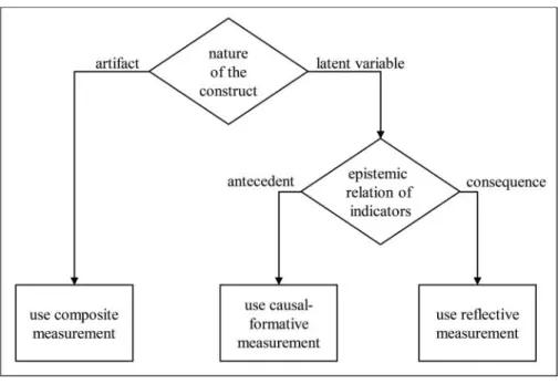
Structural equation models consist of two submodels: the measurement model, which specifies the relationships between constructs and their indicators, and the structural model, which contains the relationships between constructs. Three types of measurement models can be distinguished: composite, reflective, and causal–formative. The choice of measurement model should be driven mainly by the nature of the construct, in other words, whether a design construct or a behavioral construct is studied. Design constructs can be regarded as mixtures of elements. This suggests that they should be modeled as composites. In contrast, con-structs of behavioral sciences are typically latent variables and are traditionally modeled using reflective measurement. If causal indicators (antecedents of the construct) are avail-able in addition to the reflective indicators, an analyst can apply causal–formative measurement. Table 1 summarizes the differences between the three types of measurement models, and Figure 1 depicts the resulting decision tree.
Composite Measurement
The composite measurement model, also referred to as the composite factor model (Henseler et al. 2014), the composite– formative model (Bollen and Diamantopoulos 2015), or sim-ply the composite model, assumes a definitorial relation between a construct and its indicators. This means that the construct is made up of its indicators or elements. An example from advertising research would be brand equity as conceptu-alized by Aaker (1991): It is a construct made up of brand
awareness, brand associations, brand quality, brand loyalty, and other proprietary assets.
In composite measurement, the relationships between the indicators and the construct are not cause-effect relationships but rather a prescription of how the ingredients should be arranged to form a new entity. Nelson and Stolterman (2003, p. 119) remind us that “[a]lthough it’s true that ‘the whole is
greater than the sum its parts,’ we must also acknowledge that the wholeis ofthese parts.”
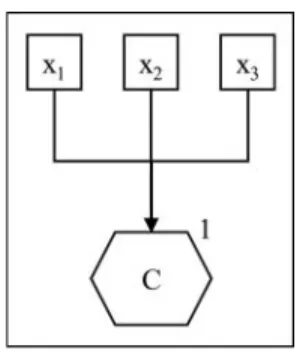
Figure 2 depicts a composite measurement model. The arrow connections between the indicators and the composite should not be regarded as causal relationships in the com-mon sense of the word causal. Rather, in terms of the four Aristotelian causes, composite measurement taps into the TABLE 1
Summary of Differences Between Types of Measurement Models
Factor Composite Measurement Reflective Measurement
Causal–Formative Measurement
Relationship between construct and indicators
The indicators make up the construct.
The construct causes its indicators.
The indicators cause the construct.
Expected correlational pattern among indicators
High correlations are common but not required.
High correlations are expected.
There is no reason to expect the measures are
correlated. Validity of scale score The scale score adequately
represents the construct.
The scale score does not adequately represent the construct.
The scale score does not adequately represent the construct.
Dealing with measurement error
Does not involve measurement error.
Takes measurement error into account at the item level.
Takes measurement error into account at the construct level.
Consequences of dropping an indicator
Dropping an indicator alters the composite and may change its meaning.
Dropping an indicator does not alter the meaning of the construct.
Dropping an indicator increases the measurement error on the construct level. Nomological net Indicators are required to
have the same consequences.
Indicators are required to have the same antecedents and consequences.
Indicators are not required to have the same antecedents and consequences.
FIG. 1. Decision tree for measurement models.
material cause instead of the efficient cause. In formal terms, the composite model regards the construct as a linear combination of its indicators, each weighted by an indicator weightw:
ξDX I
iD1
wixi (1)
Researchers who introduce a composite can be thought of as designers: They design this construct. Designers can choose whether they define the weights or let mathematical tools deter-mine the weights to achieve some kind of optimality. A typical composite construct of advertising research is the media mix: Different media can receive equal budgets, different budgets based on the decider’s experience, or different budgets based on heuristics or optimization tools (F€are et al. 2004; Reynar, Phil-lips, and Heumann 2010). Researchers using variance-based SEM typically let the software provide estimates for the weights. If the indicators are highly correlated, preset equal weights are also a viable option (McDonald 1996). In general, preset weights are the way to go if concrete weights form an integral part of the recipe of the modeled artifact.
Composite measurement models pose only a few restric-tions on the overall model. The most important restriction is that all correlations between indicators of different constructs can be explained as the product of interconstruct correlations and respective indicator loadings. Besides that, the composite measurement model does not require any assumptions about the correlations between its indicators; they can have any value. Consequently, the correlations between indicators will not be indicative for any sort of quality; applying internal consistency reliability coefficients to composite measurement models bears any meaning. Instead, composite measurement can be evaluated only in relation to its nomological net, which implies that constructs specified as composites typically require a context in which they are embedded.
Reflective Measurement
Reflective measurement models form the backbone of behavioral research. Advertising research constructs bor-rowed from consumer psychology are most often modeled in
this way. A typical example would be consumer involvement (Andrews, Durvasula, and Akhter 1990). Reflective measure-ment models are essentially common factor models, which postulate that there is a latent variable underlying a set of observable variables. In turn, each observable variable or indi-cator is regarded as an error-prone manifestation of a latent variable’s level, as expressed by the following equation:
xiDλiξCei (2)
The measurement errors are assumed to be centered around zero and uncorrelated with other variables, constructs, or errors in the model. The latent variable is not directly observ-able, but only the correlational pattern of its indicators pro-vides indirect support for its existence. Figure 3 depicts a typical reflective measurement model. The strong tie between reflective measurement and the common factor model implies that covariance-based SEM typically serves as its statistical workhorse (Bollen 1989; J€oreskog and S€orbom 1982, 1993). For a more detailed description of reflective measurement, we refer to Hair, Babin, and Krey (2017) in this issue ofJournal of Advertising.
In principle, variance-based SEM estimates composite models, not factor models. If a composite is created as a linear combination of error-prone indicators, the composite itself does contain measurement error. As a consequence, research-ers who use composites as stand-ins for latent variables will obtain inconsistent model coefficients and risk inflated Type I and Type II errors (Henseler 2012). For most types of research—except predictive research—it is indispensable to aim for consistent estimates. The solution is the correction for attenuation. It entails that the correlation between composites divided by the geometric mean of their reliabilities is a consis-tent estimate of the correlation between the factors.
There are several ways of determining the reliability of the composites. First, one can use covariance-based SEM to
FIG. 2. Composite measurement.
FIG. 3. Reflective measurement.
estimate a factor model and derive the composite’s reliability from the variance that the composite and the factor share (Ray-kov 1997). If all the weights of a composite are equal, the reli-ability can be calculated based on the factor loadings (Werts et al. 1978). Second, if a factor is embedded in a nomological net, one can exploit the fact that some variance-based SEM techniques (such as PLS Mode A) provide weights that are pro-portional to the true yet unknown correlations between the indi-cators and their common factor (Dijkstra and Henseler 2015a, 2015b). Researchers do not have to conduct a separate common factor analysis to obtain consistent estimates for the loadings.
Causal–Formative Measurement
The causal–formative measurement model (often referred to as the formative measurement model) assumes a different epi-stemic relationship between the construct and its indicators: The indicators are considered as immediate causes of the focal con-struct (Fassott and Henseler 2015). In turn, the concon-struct is seen as a linear combination of the indicators plus a measurement error. An example from advertising research would be the per-ceived interactivity of a website: This construct can be mea-sured in a causal–formative way using the indicators “active control,” “synchronicity,” and “two-way communication” (Voorveld, Neijens, and Smit 2010).
The following equation represents a causal–formative mea-surement model, where windicates each indicator’s contribu-tion toξ, anddis an error term.
ξDX I
iD1
wixiCd (3)
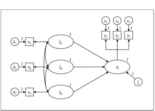
This equation strongly resembles the one for composite measurement, yet the measurement error on the construct level makes it distinct. The measurement error on the construct level implies that the construct of interest has not been perfectly measured by its formative indicators. Except for rare cases when all causes can be measured (e.g., see Diamantopoulos 2006), it is indispensable to also have a reflective measurement model; otherwise it is not possible to capture the entire content of the construct. The reflective indicators can be observed or latent as long as there are at least two reflective indicators whose correlation is fully attributable to the construct as a common cause. Figure 4 depicts a causal–formative measure-ment model.
There is some confusion in the literature about what is meant by formative measurement. Authors referring to forma-tive measurement sometimes discuss the characteristics of composite measurement and sometimes those of causal–for-mative measurement (e.g., in particular early contributions on formative measurement, such as Diamantopoulos and Winklhofer 2001; Jarvis, MacKenzie, and Podsakoff 2003). This confusion can be traced back to Edwards and Bagozzi (2000), who deliberately sought a term that characterizes both causal and definitorial relationships.
The confusion has culminated in such statements as “When an endogenous latent variable relies on formative indicators for measurement, empirical studies can say nothing about the relationship between exogenous variables and the endogenous formative latent variable” (Cadogan and Lee 2013, p. 233; for a rejoinder, see Rigdon 2014a) or variance-based SEM “is not an adequate approach to modeling scenarios where a latent variable of interest is endogenous to other latent variables in
FIG. 4. Causal–formative measurement.
the research model in addition to its own observed formative indicators” (Aguirre-Urreta and Marakas 2013, p. 776; for a rejoinder, see Rigdon et al. 2014).
The confusion can be cleared up if one carefully distin-guishes between composite measurement and causal– formative measurement. Whereas the older literature on vari-ance-based SEM tends to equate formative measurement with composite measurement (e.g., see Chin 1998; Hwang and Takane 2004), it is only recently that scholars started recom-mending the multiple indicators, multiple causes (MIMIC) model specification for causal–formative measurement in variance-based SEM, as depicted in Figure 4 (Rigdon et al. 2014). For covariance-based SEM, such types of models have been the standard for decades (e.g., see Bagozzi 1980).
Particular care is required if a construct with a causal–for-mative measurement model is meant to be explained by other constructs in the model. Researchers should then apply the lit-mus test of whether these other constructs are theorized to directly or indirectly cause the construct. In the case of a direct causal relationship, the other constructs should be added as additional formative indicators. In the case of an indirect causal relationship, the extant formative indicators mediate the effect of the other constructs. Consequently, the researcher should include effects from the other constructs on the forma-tive indicators in the model.
The Structural Model
The structural model consists of endogenous and exogenous constructs as well as the (typically linear) relationships between them. In variance-based SEM, exogenous constructs can freely correlate. The size and significance of path relation-ships are typically the focus points of the scientific endeavors pursued in empirical research.
In variance-based SEM, it is helpful to estimate two models: the estimated model, as specified by the analyst, and the satu-rated model (Gefen, Straub, and Rigdon 2011). The latter corre-sponds to a model in which all constructs can freely correlate, whereas the construct measurement is exactly as specified by the analyst. The difference lies purely in the structural model. If the estimated model is a full graph, both models will be equiva-lent. The saturated model is useful to assess the quality of the measurement model, because potential model misfit can be entirely attributed to measurement model misspecification.
In principle, it is possible for structural models to leave the comfortable realm of linear relations. In advertising research, more is not always better, but there can be optimal numbers of advertising instruments. This notion can be modeled by an inverse U-shaped relation. Another common phenomenon in advertising research is saturation. Both phenomena can be mod-eled using variance-based SEM if nonlinear terms are included in the structural model. In many cases, simple polynomial extensions can help model the typical nonlinearities in advertis-ing research (Dijkstra and Henseler 2011; Henseler et al. 2012).
A particular form of nonlinearity is moderation. One refers to a moderating effect if a focal effect is not constant but depends on the level of another construct in the model. Several approaches for modeling moderating effects using variance-based SEM have been proposed (e.g., Fassott, Henseler, and Coelho 2016; Henseler and Fassott 2010; Henseler and Chin 2010).
Model Identification
Researchers using covariance-based SEM quickly become aware of the need for identified models. The applied statistical technique can only provide unanimous estimates for the model parameters if the model is identified. Variance-based structural equation models typically do not have identification problems, because the available software packages restrict the allowed models to those that are theoretically identified.
Nevertheless, it can happen that a variance-based structural equation model is statistically underidentified. This occurs if a construct with multiple indicators is unrelated to all other con-structs in the model. In this case, any combination of indicator weights would yield the same result, namely a construct that is unrelated to the rest of the model. Analysts should avoid this situation and take care that every construct is embedded in a nomological net that consists of at least one other related vari-able in the model. If such a nomological net is not availvari-able, researchers should preset the weights or determine them by means of techniques that do not require a nomological net, such as principal component analysis (PCA).
A special identification issue is the phenomenon of sign indeterminacy, which all SEM techniques face. Sign indeter-minacy means that the statistical method can determine weight or loading estimates for a factor or a composite only jointly for their value but not for their sign. For instance, it can hap-pen that all indicators of a construct have a sign opposite to what would be expected. In covariance-based SEM, it has become customary to constrain one loading to one, dictating the orientation of the construct. Recently, this approach was partly transferred to variance-based SEM as the dominant indi-cator approach (Henseler, Hubona, and Ray 2016). For each construct, the researcher should determine one indicator—the dominant indicator—that must correlate positively with the construct. If the loading of this indicator turns out to be nega-tive, the orientation of the construct will be switched. This is achieved by multiplying its scores by¡1.
ASSESSING AND REPORTING THE RESULTS OF VARIANCE-BASED STRUCTURAL EQUATION MODELING
The fact that structural equation models consist of two sub-models has immediate implications for the way in which the results of variance-based SEM are assessed. It makes sense to analyze the relationships among the constructs only if there is
sufficient evidence of their validity and reliability. In analogy to the two-step approach for covariance-based SEM (Anderson and Gerbing 1988), a two-step approach for variance-based SEM is suggested. In a first step, the quality of construct mea-surement is determined. In a second step, the empirical esti-mates for the relationships between the constructs are examined. In the following section, we draw from new guide-lines to assess and report results of variance-based SEM (Henseler, Hubona, and Ray 2016).
Assessing Composite Measurement Models
Composites can be assessed with regard to three characteris-tics: nomological validity, reliability, and weights (composition). Composites can be regarded as prescriptions for dimension reduction (Dijkstra and Henseler 2011) and generally go along with a loss of information. Analysts face a trade-off: Should they form the composite and accept the loss of information, or continue the analysis simply using the indicators?
A generally accepted heuristic is Ockham’s razor: A model should be preferred over a more general model in which it is nested if it does not exhibit a significantly worse goodness of fit. Composites impose proportionality constraints on the cor-relations between the composite’s indicators and other varia-bles in the model. If a model with these proportionality constraints does not have a significantly worse fit than a model without them, the composite can be said to have nomological validity. If a composite has nomological validity, a researcher can infer that it is the composite that acts within a nomological net rather than the individual indicators. The concept of nomo-logical validity was developed by Cronbach and Meehl (1955) for factor models; its adaptation for the application to compos-ite measurement is new.
The statistical technique needed to test for the nomological validity of composites is confirmatory composite analysis (Henseler et al. 2014). Confirmatory composite analysis tests whether the discrepancy between the empirical correlation matrix and the correlation matrix implied by the saturated model is so small that the possibility cannot be excluded that this discrepancy is purely attributable to sampling error. The statistical test underlying confirmatory composite analysis uses bootstrapping to generate an empirical distribution of the discrepancy if the model was true (Dijkstra and Henseler 2015a). According to Zhang and Savalei (2016), this “[m]odel-based bootstrap is appropriate for obtaining accurate estimates of thepvalue for the test of exact fit under the null hypothesis” (p. 395).
In addition to the nomological validity of the composite, it is possible to determine its reliability. If a composite is mea-sured by means of perfectly observable variables, there is no random measurement error involved, and the resulting reliabil-ity of the composite equals 1. If the indicators contain a ran-dom measurement error, the composite will have imperfect reliability. In these instances, the reliability of the composite
can be determined using the following equation (Mosier 1943):
rDw0Sw (4)
In this equation for a composite’s reliabilityr,wis the col-umn vector of indicator weights, and S* is the correlation matrix of the composite’s indicators, with the respective indi-cator reliabilities in the main diagonal. Analysts facing the challenge to provide reliability estimates for each indicator could make use of respective values reported in previous stud-ies or model second-order constructs as composites of factors (van Riel et al. forthcoming).
Finally, if the weights were not preset by the analyst but freely estimated, they should be carefully studied. What is their size? What is their sign? What are their confidence inter-vals? Another point of concern should be multicollinearity among indicators (Diamantopoulos and Winklhofer 2001): High levels of multicollinearity may let indicators yield unex-pected signs or huge confidence intervals.
Assessing Reflective Measurement Models
The point of departure to assess reflective measurement models should be a model test of the saturated model (Ander-son and Gerbing 1988). In analogy to the confirmatory com-posite analysis as described in the previous subsection, reflective measurement models should be examined using con-firmatory factor analysis (CFA). If a structural equation model consists only of reflectively measured constructs, covariance-based SEM is the most versatile technique for this task. If the structural equation model also contains composites, covari-ance-based SEM is not applicable, and it is recommended that the CFA be conducted using variance-based SEM, leading to a combined confirmatory composite/factor analysis. Techni-cally, the CFA using variance-based SEM does not differ from the confirmatory composite analysis. The main difference can be found in the model-implied correlation matrix: For factor models, the implied correlation between two indicators of a factor is constrained to the product of their loadings, while these implied correlations are unconstrained for composite models.
Experience has shown that most empirical studies on mar-keting and management provide evidence against the existence of a factor model (Henseler et al. 2014). Concretely, research-ers almost always find a significant discrepancy between the empirical correlation matrix and the model-implied correlation matrix, which reflects the pattern that should be observed if the world indeed functioned according to the researcher’s model. For advertising research, the figures are quite similar, although not that bad: As Hair, Babin, and Krey (2017) point out in this issue of Journal of Advertising, about 12% of the CFAs reported in the journal exhibit factor models without signifi-cant misfit.
As a consequence of the poor test record of the factor model, many researchers lose interest in testing the hypothesis of exact fit (Zhang and Savalei 2016, p. 395), which is a wor-rying trend. They acknowledge more or less that the factor model is not (fully) correct and rely on measures of approxi-mate model fit to quantify the degree of the model’s misfit. A popular measure of approximate model fit is the standardized root mean square residual (SRMR; Hu and Bentler 1999), which has been shown to work well in combination with vari-ance-based SEM (Henseler et al. 2014). SRMR values below 0.08 typically indicate that the degree of misfit is not substan-tial (Henseler, Hubona, and Ray 2016). Instead of surrendering in the light of significant misfit and referring to measures of approximate fit, it would be wiser to investigate the sources of misfit. In terms of model diagnostics, the (standardized) resid-ual matrix is most informative to detect significant discrepan-cies between the empirical covariance matrix and the model-implied covariance matrix.
While the overall goodness-of-fit test and measures of approximate fit are informative about whether the data at hand favor a factor model, they hardly provide evidence of the qual-ity of measurement. This becomes obvious if one looks at the extreme case of a factor model whose indicators exhibit very low correlations. In this case, a factor model is unlikely to be rejected, because the discrepancy between the empirical corre-lation matrix and the model-implied correcorre-lation matrix will most likely be small. Yet it is legitimate to ask whether one was able to measure the intended factor at all. Additional qual-ity criteria have therefore been proposed.
Unidimensionality indicates whether a researcher succeeds in extracting a dominant factor out of a set of indicators. The most widely applied measure of unidimensionality is the aver-age variance extracted (AVE; Fornell and Larcker 1981). It equals the average proportion of variance explained of each reflective indicator of a latent variable. Researchers should strive for values higher than 0.5, because then there cannot be a second factor that explains as much variance as the first one. A weaker alternative is the permutation test that Sahmer, Hanafi and El Qannari (2006) proposed, which tests whether the first extracted factor explains significantly more variance than the second factor.
Discriminant validity applies if two conceptually different constructs are also statistically distinct. Fornell and Larcker (1981) operationalized this requirement as a comparison between a construct’s AVE and its squared correlations with other constructs in the model. The Fornell-Larcker criterion pos-tulates that a construct’s AVE should be higher than all its squared correlations. A new criterion for discriminant validity is the heterotrait-monotrait ratio of correlations (HTMT, proposed by Henseler, Ringle, and Sarstedt 2015). In a recent simulation study, the HTMT clearly outperforms the Fornell-Larcker crite-rion (Voorhees et al. 2016). An HTMT value significantly smaller than 1 or clearly below 0.85 provides sufficient evi-dence of the discriminant validity of a pair of constructs.
The internal consistency reliability quantifies the amount of random measurement error contained in the construct scores that serve as stand-ins for the latent variables. Consistent reliability coefficients for construct scores are Raykov’s r
(Raykov 1997) and Dijkstra-Henseler’s rho (rA, proposed by Dijkstra and Henseler 2015b). If all weights of a composite are equal, they will equal the composite reliabilityrcas proposed by Werts et al. (1978). Psychometricians recommend a mini-mum reliability value of 0.7 (Nunnally and Bernstein 1994). Finally, a researcher should ensure that each indicator loads sufficiently well on its own construct but less on other con-structs in the model. The latter can be ensured by inspecting the cross-loadings. If needed, researchers can rely on addi-tional assessment criteria implemented for covariance-based SEM (e.g., see Markus and Borsboom 2013).
Assessing Causal–Formative Measurement Models
Because causal–formative measurement models require a complementary reflective measurement model, a point of departure is the assessment of this reflective measurement. Once this is accomplished, the analyst can devote attention to the causal–formative measurement. Diamantopoulos and Winklhofer (2001) propose to assess content validity, indicator validity, indicator collinearity, and external validity of causal– formative measurement models.
Content validity is about whether the set of indicators indeed captures the full meaning of the construct. Transparent reporting of the employed indicators helps create face validity. In this way, content validity can be assessed without collecting data. Indicator validity can also be assessed before data collection by letting experts conduct a sorting task (Anderson and Gerbing 1991). If experts are able to correctly assign indicators to con-structs, one can refer to the expert validity of the indicators.
Other ways of assessing causal–formative measurement models require estimates and corresponding inference statis-tics obtained from empirical data. Concretely, indicator valid-ity applies if an indicator contributes significantly and substantially to explaining the construct. Indicator multicolli-nearity can have an adverse effect on this approach to indicator validity. Analysts are therefore advised to keep an eye on the variance inflation factors of the formative indicators.
The strongest evidence of the validity of causal–formative measurement is external validity. How much variance of the construct can be explained by the formative indicators? While there are general suggestions for threshold levels (e.g., see Henseler, Ringle, and Sinkovics 2009), it might depend on the scientific development of the construct, as well as its scientific discipline, to best identify which threshold would make sense.
Assessing Structural Models
A starting point for the assessment of structural models should be the coefficients of determination (R2values) of the
endogenous constructs. The coefficient of determination quan-tifies the proportion of variance of a dependent construct that is explained by its predictors and lies between 0 and 1. The coefficient of determination lies between 0 and 1 and quanti-fies the proportion of variance of a dependent construct that is explained by its predictors. To compare models with different numbers of independent variables estimated using differently large datasets, the adjustedR2should be applied.
Because the constructs in variance-based SEM are typically standardized, the path coefficients of the structural equation model should be interpreted like standardized regression coef-ficients: A coefficient for a path relationship between a depen-dent and an independepen-dent variable quantifies the expected increase in a dependent variable if the independent variable increases by one standard deviation and all other independent variables in the regression equation are kept constant (i.e.,
ceteris paribus). Apart from the size of a coefficient, its sign also matters, because a negative sign implies that an increase in the independent variable is accompanied by a decrease in the dependent variable.
Inference statistics for all coefficients in a structural equa-tion model are typically obtained using the bootstrap. Empiri-cal bootstrap confidence intervals are the output of choice to gauge the sampling variability of a coefficient. Alternatively, the bootstrap can provide Studenttand correspondingpvalues for one-sided and two-sided null hypothesis significance tests.
Although the path coefficients provide a first impression of the size of an effect, they are not very helpful in comparing the size of effects across models, because they are influenced by the number of other explanatory variables as well as the correlations among them. As a remedy, Cohen (1988) intro-duced the effect size,f2.f2values above 0.35, 0.15, and 0.02 can respectively be regarded as strong, moderate, and weak (Cohen 1988).
In addition to the direct effects, variance-based SEM can derive estimates for indirect effects as the departure point for the analysis of mediation (Nitzl, Roldan, and Cepeda Carrion 2016; Zhao, Lynch, and Chen 2010). The sum of the direct effect and the indirect effect(s) between two constructs is called the total effect. It is regarded as particularly useful for success factor analysis (Albers 2010).
If a researcher aims to conduct predictive research, the results need to be assessed and reported accordingly. Addi-tional desirable assessments of predictive validity are the use of holdout samples (e.g., Cepeda Carrion et al. 2016) or the tri-angulation of results using different samples (e.g., Lancelot-Miltgen et al. 2016).
EXAMPLE
To demonstrate the application of variance-based SEM in an advertising research setting, the empirical data Yoo, Donthu, and Lee (2000) reported serve as a showcase. Their empirical study of 569 individuals aims to explore the
relationships between selected marketing mix elements and the creation of brand equity. Figure 5 depicts the conceptual model. The data contain indicators of relevant advertising con-structs, and the correlation matrix is publicly available, which permits readers to completely replicate the reported analyses.2
The analyses entail CFA, SEM, and confirmatory compos-ite analysis. CFA answers the questions of whether there is evidence of the existence of nine latent variables and whether it is possible to measure them validly. SEM allows one to say something about the causal relationships among these latent variables. Confirmatory composite analysis helps answer an additional research question (not asked by Yoo, Donthu, and Lee 2000), namely whether it makes sense to create a brand equity construct as a weighted sum of the elements’ perceived brand quality, brand loyalty, and brand awareness or associations.
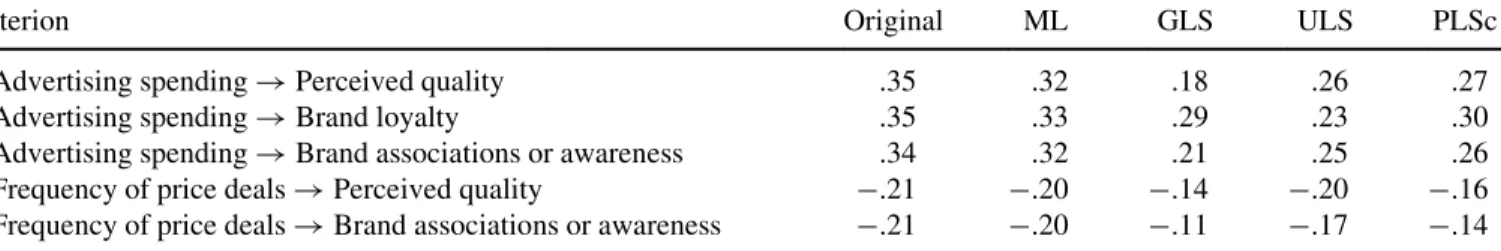
Table 2 contrasts the original values Yoo, Donthu, and Lee (2000) reported with estimates obtained with covariance-based and variance-based SEM. Yoo, Donthu, and Lee used the max-imum likelihood (ML) estimator as implemented in LISREL 8. The reanalysis makes use of three established estimators of covariance-based SEM, as implemented in the R package (R Core Team 2014) Lavaan (Rosseel 2012). Next to ML, these are generalized least squares (GLS) and unweighted least squares (ULS). Potential deviations between the original val-ues and the ML valval-ues are attributable to rounding errors (Yoo, Donthu, and Lee reported the correlation matrix with only two digits) and differences in software used. The far-right column of Table 2 contains the results from consistent PLS as implemented in ADANCO 2.0 (Henseler and Dijkstra 2015), which is currently the only variance-based SEM technique that yields consistent estimates for factor models.
Table 2 reports the outcomes from two separate analyses. The SRMR and the standardized loadings stem from a CFA, whereas the standardized path coefficients stem from SEM. The structural equation model is nested in the confirmatory factor model and has nine additional degrees of freedom (500 versus 491df).
Overall, the results obtained from variance-based SEM strongly resemble those of covariance-based SEM using the ULS estimator. Tenenhaus (2008) has already reported similar findings. The use of confirmatory composite analysis can be illustrated using the same data set, but for a model on a higher level of abstraction. Concretely, one might ask whether it makes sense to model brand equity as a second-order construct. According to Aaker’s (1991) conceptualization, brand equity is composed of perceived quality, brand loyalty, and brand awareness or associa-tions, and is therefore regarded as a composite of latent variables. Van Riel et al. (forthcoming) have shown that variance-based SEM can be used to test and consistently estimate second-order constructs in the form of composites of factors.
Figure 6 depicts two competing models, which represent two different understandings of the brand equity concept. The model on the left understands brand equity as an umbrella
term that groups three individual variables: perceived quality, brand loyalty, and brand awareness or associations. In con-trast, the model on the right regards brand equity as a compos-ite of these three factors. The second model has fewer parameters than the first, or more restrictions on the implied correlation matrix.
A confirmatory composite analysis for the model on the left yields an SRMR of 0.004 and an according HI95 value of 0.013. This means that in more than 5% of the cases one would obtain a value higher than 0.004 if the model was correct. There is therefore no reason to reject this model. In contrast, the model on the right yields an SRMR of 0.073 and an according HI95 value of 0.019, which means that it is very unlikely that the empirical data stem from a world that functions as theorized by the model.
Consequently, one should reject this model. This implies that for the empirical study of Yoo, Donthu, and Lee (2000), there is no added value in regarding brand equity as a composite of perceived quality, brand loyalty, and brand awareness or associations.
DISCUSSION
Empirical advertising research—similar to probably any other type of empirical research—strives for a logical fit between research goals and statistical techniques. Rigdon (2014b) comments that “[w]e have seen a long period where our choice of statistical tools has shaped our research goals
[. . .] In future, we need to have our choice of goals shaping
our tools” (p. 166).
FIG. 5. Example model.
TABLE 2
Comparison of Results for the Example Model
Criterion Original ML GLS ULS PLSc
Model fit in confirmatory factor analysis
SRMR .069 .069 .227 .058 .061
Standardized loadings of confirmatory factor analysis
Price PR1 .94 .94 .96 .86 .83
PR2 .74 .73 .62 .88 .91
PR3 .85 .86 .82 .77 .76
Store image IM1 .93 .93 .95 .84 .83
IM2 .82 .82 .79 .71 .70
IM3 .62 .62 .61 .78 .80
Distribution intensity DI1 .95 .96 .96 .89 .87
DI2 .93 .93 .95 .85 .84
DI3 .56 .56 .49 .69 .71
Advertising spending AD1 .89 .89 .82 .92 .92
AD2 .66 .66 .65 .65 .66
AD3 .93 .93 .97 .90 .89
Price deals DL1 .59 .58 .53 .69 .94
DL2 .94 .94 .87 .86 .73
DL3 .73 .73 .73 .68 .48
Perceived quality QL1 .87 .87 .89 .92 .95
QL2 .93 .92 .93 .88 .86
QL3 .82 .82 .81 .78 .74
QL4 .87 .86 .90 .84 .82
QL5 .84 .84 .81 .85 .86
QL6 .60 .60 .44 .66 .68
Brand loyalty LO1 .85 .85 .81 .88 .88
LO2 .94 .94 .92 .99 .99
LO3 .81 .81 .88 .74 .73
Brand associations with brand awareness AA1 .92 .92 .89 .85 .79
AA2 .92 .93 .89 .88 .84
AA3 .90 .90 .89 .87 .86
AA4 .79 .79 .74 .88 .95
AA5 .85 .85 .86 .90 .93
AA6 .66 .66 .51 .68 .67
Overall brand equity EQ1 .79 .78 .76 .80 .81
EQ2 .94 .94 .93 .95 .95
EQ3 .94 .94 .98 .94 .94
EQ4 .85 .85 .84 .84 .83
Standardized path coefficients of structural equation model
Perceived quality!Brand equity .10 .08 .05 .09 .12
Brand loyalty!Brand equity .69 .69 .73 .71 .67
Brand associations or awareness!Brand equity .07 .06 ¡.05 .05 .04
Price!Perceived quality .09 .10 .12 .11 .11
Store image!Perceived quality .32 .32 .33 .37 .36
Store image!Brand associations or awareness .33 .33 .19 .41 .41
Distribution intensity!Perceived quality .23 .23 .23 .29 .26
Distribution intensity!Brand loyalty .38 .38 .36 .46 .37
Distribution intensity!Brand associations or awareness .02 .02 ¡.06 .10 .09
(Continued on next page)
Combining design and behavioral research, empirical advertising research poses special challenges to statistical tools. It requires an SEM technique that can handle both com-posites (as the dominant model for design constructs) and fac-tors (as the dominant model for latent variables of behavioral research). Variance-based SEM is a family of techniques that fulfill this requirement.
Researchers often call for more rigor when applying vari-ance-based SEM techniques (e.g., Rigdon et al. 2014). For this purpose, methodological research has presented a wide range of extensions that enable researchers and practitioners to adequately use variance-based SEM for the purpose of their study. These advances include consistent estimates for factor models (Dijkstra 2014; Dijkstra and Henseler 2015a, 2015b), the confirmatory tetrad analysis to test the kind of measurement model and construct (Gudergan et al. 2008), the heterotrait-monotrait ratio of correlations (HTMT) to assess discriminant validity (Henseler, Ringle and Sarstedt 2015), different multigroup analysis approaches (Chin and Dibbern 2010; Sarstedt, Henseler, and Ringle 2011), testing
measurement invariance of composites (Henseler, Ringle, and Sarstedt 2016), as well as bootstrap-based tests of over-all model fit (Dijkstra and Henseler 2015a). All these changes culminate in revised guidelines for a confirmatory research use of variance-based SEM (Henseler, Hubona, and Ray 2016).
Although empirical advertising research is focused on developing and testing theories, it is sometimes also about pre-diction (Gardner 1984). Orientation toward prepre-diction has been one of the key building blocks of variance-based SEM and its most emphasized characteristic since its creation (J€oreskog and Wold 1982; Wold 1985). Recent conceptual (Chin 2010; Sarstedt et al. 2014) and empirical studies (Becker, Rai, and Rigdon 2013; Evermann and Tate 2012) substantiate the suitability of variance-based SEM for predic-tive purposes.
Future research should equip researchers with the tools and criteria they need to exploit variance-based SEM’s capabilities for predictive modeling (Shmueli 2010). The first advances in this direction have recently been presented by Cepeda Carrion TABLE 2
Comparison of Results for the Example Model (Continued)
Criterion Original ML GLS ULS PLSc
Advertising spending!Perceived quality .35 .32 .18 .26 .27
Advertising spending!Brand loyalty .35 .33 .29 .23 .30
Advertising spending!Brand associations or awareness .34 .32 .21 .25 .26
Frequency of price deals!Perceived quality ¡.21 ¡.20 ¡.14 ¡.20 ¡.16
Frequency of price deals!Brand associations or awareness ¡.21 ¡.20 ¡.11 ¡.17 ¡.14
Note. SRMRDstandardized root mean square residual; MLDmaximum likelihood; GLSDgeneralized least squares; ULSDunweighted least squares; PLScDconsistent partial least squares.
FIG. 6. Competing models of confirmatory composite analysis.
et al. (2016), Evermann and Tate (2016), and Shmueli et al. (2016). Based on these advances, more research on methods development can be expected to exploit variance-based SEM’s predictive capabilities and a more intensive use of predictive modeling in advertising research and other business and social science disciplines.
NOTES
1. I thank an anonymous reviewer for pointing out this possible source of confounding.
2. I thank Boonghee Yoo, Naveen Donthu, and Sungho Lee for per-mission to use their data in the example.
ACKNOWLEDGMENTS
The author thanks the editor, three anonymous reviewers, Gabriel Cepeda Carrion, Marko Sarstedt, Christian M. Ringle, and Jose Luis Roldan for helpful comments. The author acknowledges a financial interest in ADANCO and its distrib-utor, Composite Modeling.
ORCID
J€org Henseler http://orcid.org/0000-0002-9736-3048
REFERENCES
Aaker, David A. (1991),Managing Brand Equity: Capitalizing on the Value of a Brand Name, New York: Free Press.
Aguirre-Urreta, Miguel I., and George M. Marakas (2013), “Research Note: Partial Least Squares and Models with Formatively Specified Endogenous Constructs: A Cautionary Note,”Information Systems Research, 25 (4), 761–78.
Albers, S€onke (2010), “PLS and Success Factor Studies in Marketing,” in Handbook of Partial Least Squares, Vincenzo Esposito Vinzi, Wynne W. Chin, J€org Henseler, and Huiwen Wang, eds., Berlin: Springer, 409–25. Anderson, James C., and David W. Gerbing (1988), “Structural Equation
Modeling in Practice: A Review and Recommended Two-Step Approach,” Psychological Bulletin, 103 (3), 411–23.
———, and ——— (1991), “Predicting the Performance of Measures in a Confirmatory Factor Analysis with a Pretest Assessment of Their Substan-tive Validities,”Journal of Applied Psychology, 76 (5), 732–40.
Andrews, J. Craig, Srinivas Durvasula, and Syed H. Akhter (1990), “A Frame-work for Conceptualizing and Measuring the Involvement Construct in Advertising Research,”Journal of Advertising, 19 (4), 27–40.
Bagozzi, Richard P. (1980),Causal Models in Marketing, New York: Wiley. Becker, Jan-Michael, Arun Rai, and Edward E. Rigdon (2013), “Predictive
Validity and Formative Measurement in Structural Equation Modeling: Embracing Practical Relevance,” paper presented at the 2013 International Conference on Information Systems, Milan, Italy, December.
Bollen, Kenneth A. (1989),Structural Equations with Latent Variables, New York: Wiley.
———, and Adamantios Diamantopoulos (2015), “In Defense of Causal–For-mative Indicators: A Minority Report,”Psychological Methods, published electronically September 21, doi:10.1037/met0000056
Cadogan, John W., and Nicholas Lee (2013), “Improper Use of Forma-tive Endogenous Variables,” Journal of Business Research, 66 (2), 233–41.
Carlson, Les (2015), “The Journal of Advertising: Historical, Structural, and Brand Equity Considerations,”Journal of Advertising, 44 (1), 84–88. Cepeda Carrion, Gabriel, J€org Henseler, Christian M. Ringle, and Jose L. Roldan
(2016), “Prediction-Oriented Modeling in Business Research by Means of PLS Path Modeling,”Journal of Business Research, 69 (10), 4545–51. Chin, Wynne W. (1998), “The Partial Least Squares Approach for Structural
Equation Modeling,” in Modern Methods for Business Research, G.A. Marcoulides, ed., London: Erlbaum, 295–336.
——— (2010), “Bootstrap Cross-Validation Indices for PLS Path Model Assessment,” inHandbook of Partial Least Squares, Vincenzo Esposito Vinzi, Wynne W. Chin, J€org Henseler, and Huiwen Wang, eds., Berlin: Springer, 83–97.
———, and Jens Dibbern (2010), “A Permutation-Based Procedure for Multi-Group PLS Analysis: Results of Tests of Differences on Simulated Data and a Cross-Cultural Analysis of the Sourcing of Information System Serv-ices between Germany and the USA,” in Handbook of Partial Least Squares, Vincenzo Esposito Vinzi, Wynne W. Chin, J€org Henseler, and Huiwen Wang, eds., Berlin: Springer, 171–93.
Cohen, Jacob (1988),Statistical Power Analysis for the Behavioral Sciences, Mahwah, NJ: Erlbaum.
Cronbach, Lee J., and Paul E. Meehl (1955), “Construct Validity in Psycholog-ical Tests,”Psychological Bulletin, 52 (4), 281–302.
Diamantopoulos, Adamantios (2006), “The Error Term in Formative Measure-ment Models: Interpretation and Modeling Implications,” Journal of Modelling in Management, 1 (1), 7–17.
———, and Heidi M. Winklhofer (2001), “Index Construction with Formative Indicators: An Alternative to Scale Development,”Journal of Marketing Research, 38 (2), 269–77.
Dijkstra, Theo K. (2014), “PLS’ Janus Face: Response to Professor Rigdon’s ‘Rethinking Partial Least Squares Modeling: In Praise of Simple Methods,’” Long Range Planning, 47 (3), 146–53.
———, and J€org Henseler (2011), “Linear Indices in Nonlinear Structural Equation Models: Best Fitting Proper Indices and Other Composites,” Quality and Quantity, 45 (6), 1505–18.
———, and ——— (2015a), “Consistent and Asymptotically Normal PLS Estimators for Linear Structural Equations,”Computational Statistics and Data Analysis, 81 (1), 10–23.
———, and ——— (2015b), “Consistent Partial Least Squares Path Mod-eling,”MIS Quarterly, 39 (2), 297–316.
Edwards, Jeffrey R., and Richard P. Bagozzi (2000), “On the Nature and Direction of Relationships Between Constructs and Measures,” Psycholog-ical Methods, 5 (2), 155–74.
Evermann, Joerg, and Mary Tate (2012), “Comparing the Predictive Ability of PLS and Covariance Analysis,” paper presented at the 2012 International Conference on Information Systems, Orlando, FL, December.
———, and ——— (2016), “Assessing the Predictive Performance of Struc-tural Equation Model Estimators,”Journal of Business Research, 69 (10), 4565–82.
F€are, Rolf, Shawna Grosskopf, Barry J. Seldon, and Victor J. Tremblay (2004), “Advertising Efficiency and the Choice of Media Mix: A Case of Beer,” International Journal of Industrial Organization, 22 (4), 503–22. Fassott, Georg, and J€org Henseler (2015), “Formative (Measurement),” in
Wiley Encyclopedia of Management, Vol. 9, Marketing, Cary Cooper, Nick Lee, and Andrew Farrell, eds., Chichester: Wiley, 1–4.
———, ———, and Pedro S. Coelho (2016), “Testing Moderating Effects in PLS Path Models with Composite Variables,”Industrial Management and Data Systems, 116 (9), 1887–1900.
Fornell, Claes, and David F. Larcker (1981), “Evaluating Structural Equation Models with Unobservable Variables and Measurement Error,”Journal of Marketing Research, 18 (1), 39–50.
Gardner, Burleigh B. (1984), “Research, Measurement, and Prediction,” Jour-nal of Advertising Research, 24 (4), 16–18.
Gefen, David, Detmar W. Straub, and Edward E. Rigdon (2011), “An Update and Extension to SEM Guidelines for Administrative and Social Science Research,”MIS Quarterly, 35 (2), iii–xiv.
Gudergan, Siegfried P., Christian M. Ringle, Sven Wende, and Alexander Will (2008), “Confirmatory Tetrad Analysis in PLS Path Modeling,”Journal of Business Research, 61 (12), 1238–49.
Hair, Joseph F., Jr., Barry J. Babin, and Nina Krey (2017), “An Overview of the Use of SEM of Covariance inThe Journal of Advertising,”Journal of Advertising, 46 (1), XXX–XXX.
Henseler, J€org (2012), “Why Generalized Structured Component Analysis Is Not Universally Preferable to Structural Equation Modeling,”Journal of the Academy of Marketing Science, 40 (3), 402–13.
———, and Wynne W. Chin (2010), “A Comparison of Approaches for the Analysis of Interaction Effects between Latent Variables Using Partial Least Squares Path Modeling,”Structural Equation Modeling: An Interdis-ciplinary Journal, 17 (1), 82–109.
———, and Theo K. Dijkstra (2015), ADANCO 2.0 [Software], Kleve, Germany: Composite Modeling.
———, ———, Marko Sarstedt, Christian M. Ringle, Adamantios Diamantopoulos, Detmar W. Straub, David J. Ketchen, Joseph F. Hair, Jr., G. Tomas M. Hult, and Roger J. Calantone (2014), “Common Beliefs and Reality about PLS: Comments on R€onkk€o and Evermann (2013),” Organi-zational Research Methods, 17 (2), 182–209.
———, and Georg Fassott (2010), “Testing Moderating Effects in PLS Path Models: An Illustration of Available Procedures,” inHandbook of Partial Least Squares, Vincenzo Esposito Vinzi, Wynne W. Chin, J€org Henseler, and Huiwen Wang, eds., Berlin: Springer, 713–35.
———, ———, Theo K. Dijkstra, and Bradley Wilson (2012), “Analysing Quadratic Effects of Formative Constructs by Means of Variance-Based Structural Equation Modelling,”European Journal of Information Systems, 21 (1), 99–112.
———, Geoffrey Hubona, and Pauline Ash Ray (2016), “Using PLS Path Modeling in New Technology Research: Updated Guidelines,”Industrial Management and Data Systems, 116 (1), 1–19.
———, Christian M. Ringle, and Marko Sarstedt (2012), “Using Partial Least Squares Path Modeling in International Advertising Research: Basic Concepts and Recent Issues,” inHandbook of Research in Inter-national Advertising, Shintaro Okazaki, ed., Cheltenham: Edward Elgar, 252–76.
———, ———, and ——— (2015), “A New Criterion for Assessing Discrim-inant Validity in Variance-Based Structural Equation Modeling,”Journal of the Academy of Marketing Science, 43 (1), 115–35.
———, ———, and ——— (2016), “Testing Measurement Invariance of Composites Using Partial Least Squares,”International Marketing Review, 33 (3), 1–27.
———, ———, and Rudolf R. Sinkovics (2009), “The Use of Partial Least Squares Path Modeling in International Marketing,” inAdvances in Inter-national Marketing, Rudolf R. Sinkovics and Pervez N. Ghauri, eds., Bing-ley: Emerald, 277–320.
Hu, Li-Tze, and Peter M. Bentler (1999), “Cutoff Criteria for Fit Indexes in Covariance Structure Analysis: Conventional Criteria versus New Alter-natives,” Structural Equation Modeling: An Interdisciplinary Journal, 6 (1), 1–55.
Hwang, Heungsun, and Yoshio Takane (2004), “Generalized Structured Com-ponent Analysis,”Psychometrika, 69 (1), 81–99.
Jarvis, Cheryl Burke, Scott B. MacKenzie, and Philip M. Podsakoff (2003), “A Critical Review of Construct Indicators and Measurement Model Misspe-cification in Marketing and Consumer Research,”Journal of Consumer Research, 30 (2), 199–218.
Jensen, Morten B. (2008), “Online Marketing Communication Potential: Prior-ities in Danish Firms and Advertising Agencies,” European Journal of Marketing, 42 (3/4), 502–25.
J€oreskog, Karl G. (1978), “Structural Analysis of Covariance and Correlation Matrices,”Psychometrika, 43 (4), 443–77.
———, and Dag S€orbom (1982), “Recent Developments in Structural Equa-tion Modeling,”Journal of Marketing Research, 19 (4), 404–16.
———, and ——— (1993), LISREL 8: User’s Guide, Chicago: Scientific Software International.
———, and Herman, O. A. Wold (1982), “The ML and PLS Techniques for Modeling with Latent Variables: Historical and Comparative Aspects,” in Systems under Indirect Observation, Part I, Herman O.A. Wold and Karl G. J€oreskog, eds., Amsterdam: North-Holland, 263–70.
Kettenring, Jon R. (1971), “Canonical Analysis of Several Sets of Variables,” Biometrika, 58 (3), 433–51.
Lancelot-Miltgen, Caroline, J€org Henseler, Carsten Gelhard, and Ales Popovic (2016), “Introducing New Products That Affect Consumer Privacy: A Mediation Model,”Journal of Business Research, 69 (10), 4659–66. Lohm€oller, Jan-Bernd (1989), Latent Variable Path Modeling with Partial
Least Squares, Heidelberg: Physica.
Luxton, Sandra, Mike Reid, and Felix Mavondo (2015), “Integrated Marketing Communication Capability and Brand Performance,”Journal of Advertis-ing, 44 (1), 37–46.
McDonald, Roderick P. (1996), “Path Analysis with Composite Variables,” Multivariate Behavioral Research, 31 (2), 239–70.
Markus, Keith A., and Denny Borsboom (2013),Frontiers of Test Validity Theory: Measurement, Causation, and Meaning, New York: Routledge. Mosier, Charles I. (1943), “On the Reliability of a Weighted Composite,”
Psy-chometrika, 8 (3), 161–68.
Naik, Prasad A., and Kalyan Raman (2003), “Understanding the Impact of Synergy in Multimedia Communications,”Journal of Marketing Research, 40 (4), 375–88.
Nelson, Harold G., and Erik Stolterman, E. (2003),The Design Way: Inten-tional Change in an Unpredictable World, Englewood Cliffs, NJ: Educa-tional Technology.
Nitzl, Christian, Jose Luis Roldan, and Gabriel Cepeda Carrion (2016), “Mediation Analysis in Partial Least Squares Modeling: Helping Research-ers Discuss More Sophisticated Models,”Industrial Management and Data Systems, 116 (9), 1849–64.
Nunnally, Jum C., and Ira H. Bernstein (1994),Psychometric Theory, 3rd ed., New York: McGraw-Hill.
O’Cass, Aron (2002), “Political Advertising Believability and Information Source Value during Elections,”Journal of Advertising, 31 (1), 63–74. Okazaki, Shintaro, Hairong Li, and Morikazu Hirose (2009), “Consumer
Pri-vacy Concerns and Preference for Degree of Regulatory Control: A Study of Mobile Advertising in Japan,”Journal of Advertising, 38 (4), 63–77. ———, Barbara, Mueller, and Charles R. Taylor (2010a), “Global Consumer
Culture Positioning: Testing Perceptions of Soft-Sell and Hard-Sell Adver-tising Appeals between U.S. and Japanese Consumers,”Journal of Interna-tional Marketing, 18 (2), 20–34.
———, ———, and ——— (2010b), “Measuring Soft-Sell versus Hard-Sell Advertising Appeals,”Journal of Advertising, 39 (2), 5–20.
R Core Team (2014),R: A Language and Environment for Statistical Comput-ing, Vienna, Austria: R Foundation for Statistical Computing.
Raykov, Tenko (1997), “Estimation of Composite Reliability for Congeneric Measures,”Applied Psychological Measurement, 21 (2), 173–84. Reid, Leonard N. (2014), “Green Grass, High Cotton: Reflections on the
Evolu-tion ofThe Journal of Advertising,”Journal of Advertising, 43 (4), 410–16. Reinartz, Werner J., Michael Haenlein, and J€org Henseler (2009), “An
Empiri-cal Comparison of the Efficacy of Covariance-Based and Variance-Based SEM,”International Journal of Research in Marketing, 26 (4), 332–44. Reynar, Angela, Jodi Phillips, and Simona Heumann (2010), “New
Technolo-gies Drive CPG Media Mix Optimization,” Journal of Advertising Research, 50 (4), 416–27.
Rigdon, Edward E. (1998), “Structural Equation Modeling,” inModern Meth-ods for Business Research, George A. Marcoulides, ed., Mahwah, NJ: Erl-baum, 251–94.
——— (2014a), “Comment on ‘Improper Use of Endogenous Formative Vari-ables,’”Journal of Business Research, 67 (1), 2800–802.
——— (2014b), “Rethinking Partial Least Squares Path Modeling: Breaking Chains and Forging Ahead,”Long Range Planning, 47 (3), 161–67. ———, Jan-Michael, Becker, Arun Rai, Christian M. Ringle, Adamantios
Dia-mantopoulos, Elena Karahanna, Detmar Straub, and Theo K. Dijkstra (2014), “Conflating Antecedents and Formative Indicators: A Comment on Aguirre-Urreta and Marakas,”Information Systems Research, 25 (4), 780–84. Rosseel, Yves (2012), “Lavaan: An R Package for Structural Equation
Mod-eling,”Journal of Statistical Software, 48 (2), 1–36.
Sahmer, Karin, Mohamed Hanafi, and Mostafa El Qannari (2006), “Assessing Uni-dimensionality within the PLS Path Modeling Framework,” inFrom Data and Information Analysis to Knowledge Engineering, M. Spiliopoulou, R. Kruse, C. Borgelt, A. N€urnberger, and W. Gaul, eds., Berlin: Springer, 222–29. San Jose-Cabezudo, Rebeca, and Carmen Camarero-Izquierdo (2012),
“Determinants of Opening-Forwarding E-Mail Messages,” Journal of Advertising, 41 (2), 97–112.
Sarstedt, Marko, J€org Henseler, and Christian M. Ringle (2011), “Multi-Group Analysis in Partial Least Squares (PLS) Path Modeling: Alternative Meth-ods and Empirical Results,” inAdvances in International Marketing, Vol. 22, Marko Sarstedt, Manfred Schwaiger, and Charles R. Taylor, eds., Bing-ley: Emerald, 195–218.
———, Christian, M. Ringle, J€org Henseler, and Joseph F. Hair (2014), “On the Emancipation of PLS-SEM: A Commentary on Rigdon (2012),”Long Range Planning, 47 (3), 154–60.
Shmueli, Galit (2010), “To Explain or to Predict?”Statistical Science, 25 (3), 289–310.
———, Soumya, Ray, Juan Manuel Velasquez Estrada, and Suneel Babu Chatla (2016), “The Elephant in the Room: Evaluating the Predictive Perfor-mance of PLS Models,”Journal of Business Research, 69 (10), 4552–64. Simon, Herbert (1969),The Sciences of the Artificial, Cambridge, MA: MIT. Steenkamp, Jan-Benedict E.M., and Hans Baumgartner (2000), “On the Use of
Structural Equation Models for Marketing Modeling,”International Jour-nal of Research in Marketing, 17 (2/3), 195–202.
Tenenhaus, Arthur, and Michel Tenenhaus (2011), “Regularized Generalized Canonical Correlation Analysis,”Psychometrika, 76 (2), 257–84. Tenenhaus, Michel (2008), “Component-Based Structural Equation
Mod-elling,”Total Quality Management, 19 (7–8), 871–86.
van Riel, Allard C.R., J€org Henseler, Ildiko Kemeny, and Zuzana Saso-vova (forthcoming), “Estimating Hierarchical Constructs Using Con-sistent Partial Least Squares: The Case of Second-Order Composites of Common Factors,” Industrial Management and Data Systems, 117 (1).
Voorhees, Clay M., Michael K Brady, Roger Calantone, and Edward Ramirez (2016), “Discriminant Validity Testing in Marketing: An Analysis, Causes for Concern, and Proposed Remedies,”Journal of the Academy of Market-ing Science, 44 (1), 119–34.
Voorveld, Hilde A.M., Peter C. Neijens, and Edith G. Smit (2010), “The Perceived Interactivity of Top Global Brand Websites and its Determinants,” in Advances in Advertising Research, Vol. 1, Ralf Terlutter, Sandra Diehl, and Shintaro Okazaki, eds., Wiesbaden: Gabler, 217–33.
Werts, Charles E., Donald R. Rock, Robert L. Linn, and Karl G. J€oreskog (1978), “A General Method of Estimating the Reliability of a Construct,” Educational and Psychological Measurement, 38 (1), 933–38.
Wold, Herman O.A. (1985), “Partial Least Squares,” inEncyclopedia of Statis-tical Sciences, Samuel Kotz and Normal L. Johnson, eds., New York: Wiley, 581–91.
Yoo, Boonghee, Naveen Donthu, and Sungho Lee (2000), “An Examination of Selected Marketing Mix Elements and Brand Equity,”Journal of the Acad-emy of Marketing Science, 28 (2), 195–211.
Zhang, Xijuan, and Victoria Savalei (2016), “Bootstrapping Confidence Inter-vals for Fit Indexes in Structural Equation Modeling,”Structural Equation Modeling: A Multidisciplinary Journal, 23 (3), 392–408.
Zhao, Xinshu, John G. Lynch, and Qimei Chen (2010), “Reconsidering Baron and Kenny: Myths and Truths about Mediation Analysis,”Journal of Con-sumer Research, 37 (2), 197–206.