Control of a Buoyancy-Based Pilot Underwater
Lifting Body
Finn Haugen
Telemark University College, Kjoelnes Ring 56, N-3918 Porsgrunn, Norway. E-mail: [email protected]
Abstract
This paper is about position control of a specific small-scale pilot underwater lifting body where the lifting force stems from buoyancy adjusted with an air pocket in the lifting body. A mathematical model is developed to get a basis for a simulator which is used for testing and for designing the control system, including tuning controller parameters. A number of different position controller solutions were tried both on a simulator and on the physical system. Successful control on both the simulator and the physical system was obtained with cascade control based on feedback from measured position and height of the air pocket in the lifting body. The primary and the secondary controllers of the cascade control system were tuned using Skogestad’s model-based PID tuning rules. Feedforward from estimated load force was implemented in combination with the cascade control system, giving a substantial improvement of the position control system, both with varying position reference and varying disturbance (load mass).
Keywords: Underwater, buoyancy, air lift, position control, cascade control, feedforward control, distur-bance, estimation, Skogestad model-based controller tuning
1 Introduction
Underwater lifting operations is a common task in e.g. the offshore oil and gas production industry. This pa-per is about control of a small-scale physical pilot un-derwater lifting system.1 The lifting principle is
ad-justment of the buoyancy by controlling the amount of air in the air pocket of the lifting body. Buoyancy can provide a large lifting force with little energy, but it requires a control system. A position control system is designed and implemented to keep the body with load at a reference position. A mathematical model is de-veloped to get a basis for a simulator which is used for testing and for designing the control system, including tuning controller parameters.
Fossen(1994) and others, describe position control of underwater vehicles, but there is not much research re-ported about stabilizing underwater bodies using
buoy-1
This project was initiated and funded by the company Miko Marine, Oslo, Norway.
ancy. Several control functions were tried both on a simulator and on the physical system. The only method which worked well on the physical system was standard cascade control with positional control as the primary (master) control loop and air mass in the lift-ing body as the secondary (slave) control loop. The selected control strategy has certain similarities with the control structure described in a US patent by Ot-terblad and Dovertie (1985) where the inner loop is based on a measurement of the lifting force.2 The
sim-ulator and the control system are implemented in a LabVIEW program running with cycle time 0.02 sec on a PC.
The paper is organized as follows: The system is de-scribed in Section2. A mathematical model is derived in Section3. This model is the basis of a simulator of the system, and it is also used for design and tuning of the controllers and the observer (estimator).
Con-2
trol system design, including state observer design, is described in Section 4. Experimental results are pre-sented in Section 5. Conclusions are given in Section 6.
2 System Description
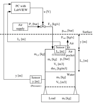
Fig. 1 shows schematically the lifting body, including the position control system. Fig. 2(left) shows a photo of the lifting body inside a water tank used for testing the position control system. Fig. 2 (right) shows the actuator which is a pneumatic control valve which ad-justs the air flow into the air pocket of the lifting body. The air flows out of the air pocket via a valve with fixed (manually adjustable) opening.
Air supply
Air pocket
Surface
Water Ps[bar]
Va[m3] ma[kg]
rhoa[kg/m3]
La[m] Air
pa[bar]
Load ml[kg] mcyl[kg]
mb[kg] Vb[m3]
patm[bar]
y [m] Fin[kg/s]
Fout[kg/s] u [V]
Sensor y [m]
Sensor La[m] (Ultrasound)
(Pressure ) PC with LabVIEW
La[m]
y [m]
Figure 1:The lifting body with load.
The lifting body positionyis measured with a sure sensor. The position is calculated from the pres-sure meapres-surement, since the position is proportional to the hydrostatic pressure. The height of the air pocket in the lifting body is measured with an ultrasound level sensor.3
It is certainly an open question whether the con-figuration shown in Fig. 1 represents optimal design. Alternative configurations are controlling the outlow, and controlling both inflow and outflow simultaneously with split-range control. However, it was not a purpose of the present project to find the optimal configuration
3
It was important that the cap of the lifting body where the sensor was mounted was isolated (we used foam plastic), to avoid disturbing sound reflections.
Figure 2:Left: Water tank with lifting body. Right: Pneumatic control valve (Samson, Type 3241, Series 250) for controlling the air flow to the cylinder.
in this sense, but to design and implement a proper position control system for the selected configuration, assuming that the principal results are transferable to a different configuration.
3 Mathematical Modeling
3.1 Variables and parameters
Variables and parameters with values are given below.
• y[m] is position of lift body. Position is zero at the water surface, and positive direction is downwards.
• flif t[N] is buoyancy lifting force.
• fh[N] is hydrodynamic drag or damping (friction)
force acting on the lifting body from the water.
• fg [N] is gravity force on the system.
• fd [N] is any independent environmental force in
addition to the forces defined above.
• mtot [kg] is total (resulting) mass to be lifted by
the lifting body.
• mb [kg] is mass of the ballast water. • mair [kg] is mass of air in air pocket
• madd = 2.0 [kg] is added (virtual) mass related
to the forced motion of water as the lifting body moves.
• mcyllif t= 2.0 [kg] is mass of the water
correspond-ing to volume taken up by the liftcorrespond-ing body in the water (causing buoyance force).
• ml = 5.0 [kg] (default value) is mass of load
at-tached to the lifting body.
• Vb [m3] is volume of ballast. • Vcyl[m3] is volume of lifting body.
• Va [m3] is volume of air pocket in lifting body. • Acyl[m2] is cross-sectional area of lifting body. • Ap [m2] is a cross-sectional area parameter used
to calculatefd.
• Lcyl= 0.6 [m] is length of lifting body. • d= 0.2 [m] is lifting body diameter.
• La [m] is height of air pocket in lifting body. • ρa [kg/m3] is density of air in air pocket (at the
present depth).
• ρaatm = 1.2 [kg/m
3] is density of air at the surface
(atmospheric pressure).
• ρw= 1025 [kg/m3] is water density.
• Fin [kg/s] is air mass flow into lifting body from
the compressor, through the control valve.
• Fout [kg/s] is air mass flow out from lifting body
through outlet valve.
• Kh = 0.004 [N/(m/s)2] is hydrodynamic drag or
damping (friction) force.
• Kv= 250 [kg/s] is valve constant of inlet (control)
valve.
• Kvout is valve constant of outlet (manual) valve.
• patm [Pa] is atmospheric air pressure.
• ps[Pa] is the pressure of the air out from air
com-pressor (air supply).
• ∆pin[Pa] is pressure drop across air inlet valve. • ∆pout [Pa] is pressure drop across air outlet valve. • ∆patm= 101000 [Pa] is atmospheric pressure. • u[V or %] is valve control signal.
• g= 9.81 [m/s2] is gravity constant.
The parametersKhandKvout were adjusted
manu-ally in a simulator until the simulated position showed the similar response as the measured position. The parameter madd was given an assumably reasonable
value.
3.2 Mathematical modelling
A mathematical model describing the motion of the lifting body was developed from the following modeling principles:
• Equation of motion of the lifting body with load
• Mass balance of the air in the air pocket of the lifting body
Modeling details are given in the following sections.
3.2.1 Equation of motion
Applying Newton’s Second Law gives
mtoty¨=−flif t−fh+fg+fd (1)
mtot in eq. (1) is described in detail below.
mtot=mb+madd+mcyl+ml (2)
where
mb = ρwVb (3)
Vb = Vcyl−Va (4)
Va =
ma
ρa
(5)
mais given by the mass balance of the air in the lifting
body, cf. eq. (20) below. Now, eq. (1) becomes
mtot=ρw
Vcyl−
ma
ρa
+madd+mcyl+ml (6)
where
Vcyl=AcylLcyl (7)
In eq. (6),ρais a function of depthygiven by the Gas
Law:
ρa(y) =
p(y)
RT (8)
Ris the specific gas constant, andTis the temperature. Assuming constantT, eq. (8) gives
ρa(y)
pa(y)
= ρa(0)
pa(0)
≡ρaatm
patm
(9)
Here,
pa(y) =patm+ρwg(La+y) (10)
Now eq. (9) gives
ρa(y) = ρaatm
pa(y)
patm
(11) = ρaatm
1 +ρwg(La+y)
patm
Here we will make the assumption that
y≫La (13)
which will hold when the lifting body is at relatively large depths. This implies
ρa(y)≈ρaatm
1 +ρwgy
patm
(14)
which is used in eq. (6). Each of the terms at the right side of eq. (1) are now described: In eq. (1), the lifting forceflif tis given by
flif t=ρwVag (15)
where
Va = AcylLa (16)
Acyl =
πd2
4 (17)
In eq. (1),
fh=Kh
dy dt
dy dt
(18)
whereKh is adjusted manually during experiments.
In eq. (1),
fg = ml+mcyl−mcyllif t
g (19)
where the termmcyllif tg is the buoyance force due to
the lifting body itself being submerse.
3.2.2 Mass balance of air in air pocket
The massma of the air in the air pocket of the lifting
body is varying. A mathematical model ofmais given
by the following mass balance of the air in the lifting body:
˙
ma=Fin−Fout (20)
The air mass inflowFinand the air mass outflowFout
are described in detail in the following.
Modeling the air inflow
Finis assumed to be a controllable (adjustable)
in-put variable. In practice the specified Fin is obtained
by manipulating the control signal uto the inlet con-trol valve. uis a voltage in the range of [0 – 5V] which will be represented with a percent value in the range of [0 – 100%], with a linear relation between the ranges.
Finis ideally given by the valve equation:
Fin=Kvfv1(u) s
∆pin
patm
(21)
∆pinis the pressure drop across the valve:
∆pin=ps−pa (22)
Typically,
ps≫pa (23)
Hence,
Fin≈Kvfv1(u)
r p
s
patm
(24)
fv1(u) is the valve flow characteristic function
normal-ized with values between 0 and 1. The valve used in this project has an equal percentage valve characteris-tic function. However, since we have an air flow meter installed in the rig, we have decided to model the valve with experimental relation between control signal and flow. Fig. 3shows the air flowFin [kg/s] as a function
of the valve control signalu[%]. The supply pressure wasps= 1 bar. The circles are experimental data, and
the lines are just linear interpolations.
0 10 20 30 40 50 60
0 0.2 0.4 0.6 0.8 1 1.2 1.4 1.6 1.8
2x 10
−3
Flow [kg/s]
Valve control signal, u [percent]
Figure 3:Air flowFin [kg/s] as a function of the valve
control signal.
In the project weinverted this valve function by us-ing table-lookup based on linear interpolation between the tabular data. Hence, for any specified flow Fin,
the table-lookup give the valve control signaluneeded to obtain that flow. One convenient consequence of this is that the nonlinear valve can be represented by a linear valve with flow Fin as the control signal (or
manipulating variable).
Modeling the air outflow
In eq. (20) the air mass outflow Fout through the
valve, which has fixed opening, is modelled as
Fout=Kvout
s |∆pout|
patm
where ∆pout is the pressure drop across the valve.
sign(∆pout) is the sign function, which has value 1 if
the argument (∆pout) is positive, and −1 if the
argu-ment is negative. ∆pout is given by
∆pout=ρwgLa (26)
4 Control System Design
4.1 Introduction
Several controllers were designed and tried out both on the simulator (based on the model described in Section 3) and the real system. The application of these con-trollers is described briefly below. All of the concon-trollers worked on a simulator, but the only method which worked well and without problems on the physical sys-tem was cascade control, which also was enhanced with feedforward from estimated load force. (Section 4.2 describes details of the cascade control system.) One practical problem with the physical system is that the height of the water tank is relatively small as the height is about 1.5 m. Therefore, the lifting body with load mass easily reached physical constraints during exper-iments. Some of the other controllers might work well too under different physical conditions.
Certainly, it is benefical if the control task is satis-factorily solved with a “standard” controller and this turned out to be the case in the present application (with cascade control).
Below is a short description of the application of the various controllers:
• Feedback linearization in combination with
a Kalman filter which estimates the state
variables. The state variables are the lifting
body position and velocity and the mass of air in the air pocket. Basically, with this controller, nonlinear (and linear) terms of the process model are cancelled out. The resulting process model is linear and simple (three integrators in series). A linear pole-placement controller for this model, augmented with an integrator in the controller to obtain integral control action, was designed. Al-though the controller worked excellently with the simulated system (with no model errors assumed), it was not able to stabilize the real system. This is probably because of too large sensitivity to model errors. Model errors are particularly apparent when the system reaches physical constraints, but this was not analyzed in detail. Furthermore, the sensitivity to an erroneous estimate of mass of air in the air pocket in the lifting body is probably large. The mass of air is closely related to the lifting force. Intuitively, an erroneously calculated
lifting force may cause problems for stabilization of the body position.
• Linear feedback control with pole-design in
combination with a Kalman filter which
es-timates the state variables. This controller is
based on a simplified process model being valid close to a certain operating point, which was se-lected as the “static” operating point, where the body is at rest (this is the most critical operating point regarding stability). This controller worked well on the simulated system, but not on the real system, probably because of the same reasons as for Feedback linearization (see above).
• PID controller with lead element in series
with the PID controller. Ordinary PID
con-trol could not stabilize the system at all due to the dynamic properties of the process which is roughly a triple integrator (three integrators in series), at least at a static operating point where damping hydrodynamic drag force (as modeled in this project) is zero. Position is integral of velocity which is integral of acceleration which is propor-tional to mass of air in air pocket, and this mass is roughly the integral of air inflow. A PID controller can stabilize a double integrator, but not a triple integrator because a phase lead of more than 90 degrees provided by the controller is needed, and the PID controller can not add more positive phase (lead action) than 90 degrees (ideally) to the con-trol loop. Therefore, a lead-lag element with dom-inant lead action providing the additional phase lead was included in the controller, succeeding the PID controller. Actually, this controller was able to stabilize the real system, but it became unsta-ble after small disturbances (perturbations), so it was concluded that the controller was not suffi-ciently robust. Also, the control signal was very noisy, due to the derivative action corresponding to the phase lead action. This noise makes the stabilization difficult.
• PID controller together with body
acceler-ation feedback, where the acceleracceler-ation was
estimated with a state observer. The purpose
implemented in this project. (So, it is unclear if control using acceleration measurement works bet-ter than using acceleration estimate.)
• Cascade control, with feedforward from
es-timated load force. The primary (master) loop
of the cascade control system realizes position trol, and the secondary (slave) loop realizes con-trol of air height in the air pocket of the lifting body. Cascade control is “industry standard”, and it worked successfully without problems in this project. In the controller design, the clue is to identify the secondary process variable to be mea-sured. The process model was a great help to this end as the model revealed that the state variables are lifting body position and velocity and mass of air in the air pocket. The primary controller is of course based on the lifting body position, and indirectly on velocity which is calculated by the derivative action of the PID controller. The secondary controller is based on the third process state variable - the air mass. (The cascade con-troller resembles state-variable feedback, which is known to be able to stabilize “any” process.) How-ever, this mass is not measured directly. Instead, a closely related variable, namely the height of the air pocket, is measured. The cascade controller was enhanced with feedforward from estimated load force. Details about the cascade controller and is given in Section4.2, and details about es-timation of load force and feedforward from the force estimate is given in Sections4.3and4.4, re-spectively.
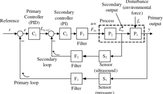
4.2 Cascade control
4.2.1 Control system structure
C1 C2 P2 P1
S2
S1
u=
Fin y
e
r La
Sensor (ultrasound) Primary
Controller (PID)
Secondary controller (PI)
Primary loop Secondary
loop
Secondary output
Primary output Process
Reference
F1
Filter F2
F3
Sensor (pressure) Filter
Filter
Disturbance (environmental
force)
La,ref
fe
Figure 4:Cascade control system.
Fig. 4shows a block diagram of the cascade control system based on feedback from measured underwater lifting body positiony(this feedback is of course oblig-atory in a positional control system) and measured air
height La of the air pocket. Thus, two sensors were
implemented.
Since a mathematical model exists, it was tempting to try feedback from estimated La as an alternative
to feedback from measured La. However, this did not
work well on the physical system as the control sys-tem became unstable. The syssys-tem relies on accurate knowledge about La, and an estimate can not replace
the measurement in this case.
One practical benefit of cascade control compared with more complex control structures is that the user can manipulate the amount of air (the secondary or internal process variable) directly during testing etc. This is done by setting the primary controller into man-ual mode, and manipulating the manman-ual control signal of the primary controller which is the setpoint of the secondary controller.
4.2.2 Signal filters
Lowpass (time-constant) filters were implemented in LabVIEW to smooth theymeasurement – this is filter F1 in Fig. 4– and theLa measurement – this is filter
F2in Fig. 4. Also, a lowpass filter was implemented to
smooth the control signal,u=Fin– this is filter F3in
Fig. 4. In the experiments the F1 filter was used with
time-constant of 0.1 s because that measurement was somewhat noisy. The F3 filter was used with a
time-constant of 0.1 s to get a smooth control signal to the valve. The F2filter was actually not used (i.e. its
time-constant was set to zero) because the measurement of
La contained little noise.
4.2.3 Controller tuning
The master PID controller and the slave PI controller were both tuned using the mathematical model of the system.4 Both controllers were tuned from
specifica-tions of the response-time (time-constants) of the re-spective control loops using Skogestad’s method of PID controller tuningSkogestad(2003).
Tuning of the primary controller (PID) The primary control variable isLa, which is used as the setpoint of
the secondary loop. It is assumed that the dynamics of the secondary loop which controlsLais so fast relative
to the dynamics of the primary loop that the setpoint of
La is obtained approximately immediately. Thus, the
process model used as the basis for tuning the primary loop is as follows:
mtoty¨=−flif t−fh+fg+fd (27) 4
where
mtot = mb+madd+mcyl+ml (28)
mb = ρw(Vcyl−AcylLa) (29)
flif t = ρwAcylgLa (30)
fh = Khy˙|y˙| (31)
fg = ml+mcyl−mcyllif t
g (32)
To tune the primary PID controller, a transfer func-tion model withLa as input andyas output is useful.
This model can be derived by rigorous linearization of a nonlinear state-space model corresponding to eq. (27). Alternatively, it can be derived as follows: Since the hydrodynamic damping forcefh given by eq. (31) has
its minimum value of zero when the speed ˙yis zero, the most critical operating point – which should be used for controller tuning – is at ˙y = 0. From the model eqs. (27) – (32), the relation betweenLa andy at this
operating point is
mtoty¨(t) =−ρwAcylgLa(t) (33)
From eq. (33) the transfer function from La to y is
found as
y(s)
La(s)
=P1(s) = K1
s2 (34)
where the gainK1 is
K1=−ρwAcylg
mtot
(35)
P1(s), which is a “double integrator”, can be con-trolled with a PID controller. To tune the con-troller parameters, Skogestad’s method, also denoted the SIMC method5,Skogestad(2003) is used:
Kp =
1 4K1(TC1)
2 (36)
Ti = 4TC1 (37)
Td = 4TC1 (38)
where TC1 is the user-specified time-constant of the
control system (the primary loop). In general for the double-integrator being tuned with Skogestad’s for-mulas, it turns out that the actual (simulated) time-constant is about three times larger than the specified
TC1. But sinceTC1 has to be manually adjusted on the
real system, this inaccuracy is not important. TC1 is
the only tuning parameter of the PID controller. TC1
can be selected by trial-and-error on a simulator, and should be further tuned on the real control system. It was found that
TC1 = 2.5 s (39)
5
SIMC = Simple Internal Model Control
was a good value on the simulator and on the real sys-tem.
Skogestad’s tuning rule assumes a serial PID con-troller function, which has the following transfer func-tion (assuminguis the control signal andeis the con-trol error):
u(s) =La(s) =Kps
(Tiss+ 1) (Tdss+ 1) Tiss
e(s) (40)
whereKps,Tis, andTds are the controller parameters
given by eqs. (36) – (38). However, the PID con-troller used in this project actually implementes a par-allel PID controller, which has the following transfer function:
u(s) =La(s) =
Kpp+
Kpp Tips
+KppTdps
e(s) (41)
To transform the serial PID settings to parallell PID settings, we apply the following serial-to-parallel trans-formationsSkogestad(2003):
Kpp = Kps
1 +Tds Tis
= 1
4K(TC1) 2
1 + 4TC1
4TC1
= 1
2K1(TC1)
2 =Kp (42)
Tip = Tis
1 +Tds Tis
= 4TC1
1 + 4TC1
4TC1
= 8TC1=Ti (43)
Tdp = Tds
1 1 +Tds
Tis
= 4TC1
1 1 +4TC1
4TC1
= 2TC1 =Td (44)
Tuning of the secondary controller (PI) The sec-ondary control loop controlsLa. The setpoint isLaref
which is equal to the output of the primary controller. The control variable calculated by the secondary con-troller is Fin, which is applied to the control valve.
The mathematical model of the process that the sec-ondary controller controls, is given by eq. (20) which is repeated here:
˙
ma=Fin−Fout (45)
The relation betweenLa andma is given by
ma=ρaVa =ρaAcylLa (46)
Above, the air density ρa is given by eq. (14).
calculated by eq. (14) and is therefore known. Fur-thermore, we can assume that the outflow Fout is a
disturbance. Then, the model of the process that the secondary controller controls, is
ρaAcylL˙a=Fin−Fout (47)
The transfer function from control variableFinto
pro-cess output variableLa becomes
La(s)
Fin(s)
=P2(s) = K2
s (48)
which is an integrator. The gainK2is
K2= 1
ρaAcyl
= 1
ρaatm
1 +ρwgy
patm
Acyl
(49)
To tune the secondary controller for a process given by eq. (48), we use Skogestad’s method Skogestad (2003):
Kp=
1
K2TC2
(50)
Ti = 1.5TC2 (51)
Td= 0 (52)
where TC2 is the user-specified time-constant of the
secondary control system. It was found that
TC2 = 1.0 s (53)
is a good value on the simulator and on the real system.
4.3 Estimation of load force
An estimator of the load force was implemented. The force estimate was used in feedforward control as ex-plained in Section 4.4. The estimator was designed as an observer with specified dynamics, see Goodwin et al.(2001). The design is described in the following. The mathematical model which is the basis of the estimator is
mtoty¨=−ρwAcylgLa
| {z }
flif t
−Khy˙|y˙| | {z }
fh
+fe (54)
where fe is the environmental or disturbance force to
be estimated. fewill actually represent any force that
is not included in the model, or that is not modelled correctly. It is assumed that fe is unknown without
any information about its variation. An appropriate model which describesfe is therefore
˙
fe= 0 (55)
It is assumed that all variables and parameters except
feare known. In particular,La is known from its
mea-surement. In applications where the mtot varies
sub-stantially, it may be necessary to estimate it, but this has not been done in the present project.
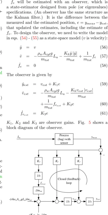
fe will be estimated with an observer, which is
a state-estimator designed from pole (or eigenvalues) specifications. (An observer has the same structure as the Kalman filter.) It is the difference between the measured and the estimated position,e=ymeas−yest,
that updated the estimates, including the estimate of
fe. To design the observer, we need to write the model
in eqs. (54) - (55) as a state-space model (vis velocity): ˙
y = v (56)
˙
v = −ρwAcylg
mtot
La−
Khy˙|y˙|
mtot
+ 1
mtot
fe (57)
˙
fe = 0 (58)
The observer is given by ˙
yest = vest+K1e (59)
˙
vest = −
ρwAcylg
mtot
La−
Khvest|vest|
mtot
+ 1
mtot
feest+K2e (60)
˙
feest = K3e (61)
K1, K2 and K3 are observer gains. Fig. 5 shows a block diagram of the observer.
Process (bag) with
sensor
1/s
La ym eas
K3
1/s
1/mtot fe,est
K1
1/s K2
yest vest
_
-(Khvest|vest|)/mtot -(rhowAcylgLa)/mtot
Closed (feedback) loop
Figure 5:The observer which is used to estimate the environmental force fe. (1/s is the transfer
function of an integrator.)
of the observer. It can be shown that the characteristic polynomial of this loop is
cobs(s) =s3+K1s2+K2s+
K3
mtot
(62) The observer poles were selected as Butterworth poles Franklin and Powell(1980). Butterworth poles give a step response with a slight overshoot and good damp-ing. (Of course, other poles configurations are possi-ble.) Butterworth poles of a normalized third order system correspond to the following characteristic poly-nomial:
cbutternorm(s) =c3s
3+c2s2+c1s+c0 (63)
where
c3= 1; c2= 2; c1= 2;c0= 1 (64)
If we specify that the system has response-time6T r
ap-proximately equal to 3T, the Butterworth polynomial becomesHaugen (2010)
cbutter1(s) =c3(T s) 3
+c2(T s)2+c1(T s) +c0 (65) which has the same roots as
cbutter(s) =s3+
c2 c3
1
Ts
2+c1 c3
1
T2s+
c0 c3
1
T3 (66)
Comparing cobs(s) and cbutter(s) gives the following
formulas for the observer gains:
K1 = c2
c3
1
T (67)
K2 = c1
c3
1
T2 (68)
K3 = c0
c3
1
T3mtot (69)
The algorithm of the observer ready for progamming is derived by discretizing the observer formulas in eqs. (59) – (61) using Forward differentiation approxima-tion. The resulting observer formulas are as follows:
yest(tk+1) =yest(tk) +h[vest(tk) +K1e(tk)] (70)
vest(tk+1) =vest(tk)
+h "
−ρwAcylg
mtot La(tk)−
Khvest(tk)|vest(tk)|
mtot
+ 1
mtotfeest(tk) +K2e(tk) #
(71)
feest(tk+1) =feest(tk) +hK3e(tk) (72)
where
e(tk) =ymeas(tk)−yest(tk) (73)
his the time-step (0.02 s). The observer response-time
Trwas set to 0.8 s. 6
Here, response-time means time to reach 63% of steady-state value, similar to the definition of time-constant for first order systems.
4.4 Feedforward from estimated load force
From eq. (54) we get the following feedforward con-troller function:
Laf f =
1
ρwAcylg
feest (74)
which is added to the control output from the primary controller, Laprim, so that the total reference to the
secondary controller becomes
Laref =Laprim+Laf f (75)
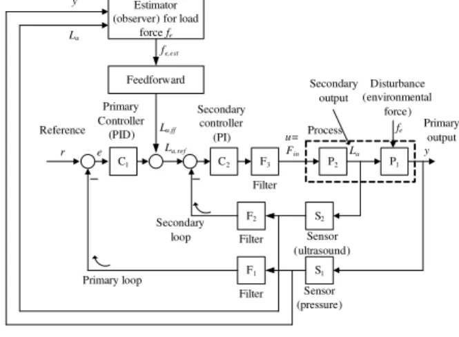
Fig. 6 shows the structure of the cascade control sys-tem including estimator (observer) and feedforward model.
C1 C2 P2 P1
S2
S1
u=
Fin y
e
r La,ref La
Sensor (ultrasound) Primary Controller (PID) Secondary controller (PI) Primary loop Secondary loop Secondary output Primary output Process Reference F1 Filter F2 F3 Sensor (pressure) Filter Filter Disturbance (environmental force) fe Feedforward Estimator (observer) for load
force fe fe,est
La ,ff y
La
Figure 6:The structure of the cascade control system including estimator (observer) and feedfor-ward model.
5 Experimental Results
5.1 Introduction
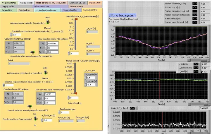
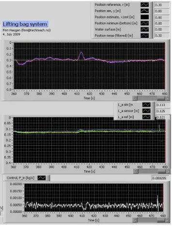
Experiments were run with cascade control with feed-forward from estimated load force. Fig. 7 shows the available parameters of the control system. The exper-iments reported in the next sections are about
• position reference tracking, where the reference was changed as a ramp, and
Figure 7:Controller settings of the cascade control sys-tem in LabVIEW.
5.2 Position reference tracking
Fig. 8 shows the lifting body position reference (set-point) r and measurement y, together with air body height reference Laref and measurementLa. Also the
control signalFinapplied to the control valve is shown.
The position reference was initially 0.3 m, and then changed as a ramp downwards with slope 0.005 m/s, and then upwards with the same slope. When the reference was constant (before the ramping started), the maximum position control error was approximately 0.02 m, due to various sources of noise in the system (the error is zero in an ideal, noise-free system). During the ramping, the maximum steady-state error was ap-proximately 0.03 m. In an earlier experiment, cascade control without feedforward from estimated force was run. The control error was substantially larger than with feedforward. (No plots are shown here.) The superior control at using feedforward from estimated load was somewhat surprising, because the load was not changed during these experiments. It seems that the load estimate encapsulates the effects of various sources causing the control error to become different from zero.
Figure 8:Cascade control with feedforward from esti-mated load force: Ramped changes of the po-sition reference.
5.3 Disturbance (load) compensation
Fig. 9shows the responses as a mass load of 0.5 kg was suddenly added to the body at time 360 s, and then suddenly removed from the body at time 410 s. The maximum response in the lifting body after the load was added was 0.08 m, while the maximum response after the load was removed was 0.12 m – an average of 0.10 m. It took about 15 sec until the position was back at the reference.
In another similar experiment without feedforward the maximum response in the lifting body was 0.23 m, and position was back at the reference after 250 sec. Thus, disturbance compensation was substantially improved with feedforward.
6 Conclusions
Figure 9:Cascade control with feedforward from esti-mated load force: A load mass of 0.5 kg was added at time 360 s, and then removed at time 410 s.
The cascade control system is based on feedback from both measured lifting body position and measured air height in the lifting body. Thus, two sensors were im-plemented. Both the master PID controller and the slave PI controller were tuned using Skogestad’s model-based PID tuning rules. The only specifications for Skogestad’s tuning is the time-constant of the control loop. The tunings were tried on the simulator before being applied to the real system, and there was hardly any need to retune the controllers. Feedforward from estimated load force was implemented with the cas-cade control system. At constant position reference the maximum control error was 0.02 m. At ramping posi-tion reference of slope 0.005 m/s the maximum control error was 0.03 m. At constant reference but with a suddenly added load mass of 0.5 kg the maximum con-trol error was 0.10 m in average (0.08 m after the load was added, and 0.12 m after the load was removed), and the position was back at the reference after 15 s. Experiments with cascade control but without feedfor-ward gave a control error that was substantially (many times) larger, both at changing reference and at chang-ing disturbance (load mass).
Acknowledgments
I want to express my thanks to Eivind Fjelddalen at Telemark University College who constructed the test rig, and to Claus Christian Apneseth at Miko Marine who initated the project and gave valuable inputs and comments as the project evolved.
References
Fossen, T. Guidance and Control of Ocean Vehicles. John Wiley & Sons Ltd., 1994.
Franklin, G. and Powell, J.Digital Control of Dynamic Systems. Addison-Wesley, 1980.
Goodwin, C., Graebe, S., and Salgado, M. Control System Design. Prentice-Hall, 2001.
Haugen, F. Advanced Dynamics and Control. TeachTech, 2010.
Otterblad, S. and Dovertie, R. Lifting body for diving. 1985. US Patent number 4,498,408.
![Figure 3: Air flow F in [kg/s] as a function of the valve control signal.](https://thumb-eu.123doks.com/thumbv2/123dok_br/18202532.333664/4.892.85.436.371.568/figure-air-flow-f-function-valve-control-signal.webp)