J. Braz. Comp. Soc. vol.10 número3

A Modeling Methodology

for Hierarchical

Control System and its Aplication

Abstract

Current and future computerized systems and in-frastructures are going to be based on the layering of dif-ferent systems, designed at difdif-ferent times, with difdif-ferent technologies and components and difficult to integrate. Control systems and resource management systems are in-creasingly employed in such large and heterogeneous en-vironment as a parallel infrastructure to allow an effi-cient, dependable and scalable usage of the system com-ponents. System complexity comes out to be a paramount challenge to solve from a number of different viewpoints, including dependability modeling and evaluation. Key directions to deal with system complexity are abstraction and hierarchical structuring of the system functionalities. This paper addresses the issue of an efficient dependabil-ity evaluation by a model-based approach of hierarchical control and resource management systems. We exploited the characteristics of this specific, but important, class of systems and derived a modeling methodology that is not only directed to build models in a compositional way, but it also includes some capabilities to reduce their solution complexity. The modeling methodology and the resolu-tion technique are then applied to a case study consisting of a resource management system developed in the context of the ongoing European project CAUTION++. The re-sults obtained are useful to understand the impact of sev-eral system component factors on the dependability of the overall system instance.

Keywords: Modeling Methodology, Quality of Ser-vice, Modular & Hierarchical Modeling, Petri Nets, Valida-tion, Control Systems & Infrastructures

1 I

Current and future computerized systems and infra-structures are based more and more on the layering of dif-ferent systems, designed in difdif-ferent times, with difdif-ferent technologies and components and difficult to integrate. Control systems and resource management systems are in-creasingly employed in such large and heterogeneous en-vironment to allow an efficient, dependable and scalable usage of the system components. In such landscape, sys-tem complexity comes out to be a paramount challenge to cope with from a number of different points of view, includ-ing dependability evaluation. Key directions to deal with system complexity are abstraction and hierarchical struc-turing of the system functionalities.

System evaluation is a key activity of fault forecast-ing, aimed at providing statistically well-founded quantita-tive measures of how much we can rely on a system. In particular, system evaluation achieved through modelling supports the prediction of how much we will be able to rely on a system before incurring the costs of building it. It is therefore a very profitable evaluation approach to be em-ployed since the very beginning of a system development activity.

Most of the new challenges in dependability model-ling are connected with the increasing complexity and dynamicity of the systems under analysis. Such complexity needs to be attacked both from the point of view of system representation and of the underlying model solution. In fact, the state space explosion is a well known problem in model-based dependability analysis, which strongly limits the

ap-Paolo Lollini and Andrea Bondavalli

University of Florence Dip. Sistemi e Informatica

Viale Morgagni 65 50134 - Florence - ITALY {lollini – a.bondavalli}@dsi.unifi.it

Felicita Di Giandomenico

Italian National Research Council ISTI Dept.

plicability of this method to large complex systems, or heavily impacts on the accuracy of the evaluation results when simplifying assumptions are made as a remedy to this problem. Modular and hierarchical approaches have been identiffied as effective directions. Resorting to a hierarchi-cal approach brings benefits under several aspects, among which: i) facilitating the construction of models; ii) speed-ing up their solution; iii) favorspeed-ing scalability; iv) masterspeed-ing complexity (by handling smaller models through hiding, at one hierarchical level, some modeling details of the lower one). At each level, details of the architecture and of the status of lower level components are not meaningful, and only aggregated information should be used. Therefore, information of the detailed models at one level should be aggregated in an abstract model at a higher level. Important issues are how to abstract all the relevant information of one level to the upper one and how to compose the derived abstract models. However, it is important to underline that the modularity of the modelling approach alone cannot be truly effective without a modular solution of the defined models.

In this paper, we focus on the class of control and resource management systems. To cope with their increas-ing complexity, such systems are typically developed in a hierarchical fashion: the functionalities of the whole sys-tem are partitioned among a number of subsyssys-tems work-ing at different levels of a hierarchy. At each level, a sub-system has knowledge and control of the portion of sub-system under its control (lower levels), while it acts just as an ac-tuator with respect to the higher level subsystems. In this organization, the flow of the information goes vertically from one level to the other, but not horizontally inside the same level. More precisely, the flow of decision taking goes from the bottom to the top, while the flow for decision actuation goes from the top to the bottom. Here we are interested in modeling and evaluating the system behavior with refer-ence to a unidirectional flow (be it for decision taking or for decision actuation). To improve dependability, fault toler-ance measures may be taken at each level, typically intro-ducing interface checks to cope with erroneous inputs and/ or outputs and internal checks to cope with faults during the internal computation. We exploited the characteristics of this specific, but well representative, class of systems and derived a modeling methodology that is not only di-rected to build models in a compositional way, but it also includes some capabilities to reduce their solution com-plexity. To show how it works, in the second part of the paper we applied the methodology to a case study, which consists of a resource management system developed in-side the CAUTION++ project [1].

The rest of this paper is organized as follows. Sec-tion 2 provides some preliminaries on the considered class of systems. Section 3 outlines the modeling approach. Sec-tion 4 presents the multi-stage system instance considered in the analysis. In Section 5 the models set-up for the se-lected CAUTION++ instance are discussed, while the re-sults of the numerical evaluation are provided in Section 6. Finally, conclusions are in Section 7.

2 S

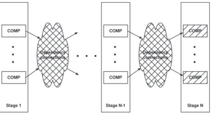
The class of systems we focus on consists of a set of hardware or software components (the Comp boxes), which are grouped in “stages” (Stage 1, ..., Stage k, ..., Stage N), as shown in Figure 1.

Figure 1: Class of systems with “multi-stage” representation

Components at a certain stage may interact with oth-ers at an higher level through some “Dependency connec-tions”. Each connection identifies a dependency between two system components: a component A is connected to a component B (A

→

From the general system depicted in Figure 1 and following the dependency connections from a root compo-nent back to the leaves of the graph, a number of individual subsystems structured in a hierarchical fashion may be de-rived, equal to the number of root components.

As already discussed earlier, a component at stage k may interact only with those at stages k-1 and k+1 and these dependencies are unidirectional, from the lower stage to the higher one. A dependency between one component at stage k and more than one component at stage k+1 is not explicitly considered as it is equivalent to consider some (logical) replications of the component at stage k, each one interacting with only one component at stage k+1. In do-ing this we make the assumption that, if a component is used in computing two or more outcomes, its behavior is independently modeled in each context. This means that the behavior of each replica does not depend on the behav-ior of the others.

The components in a stage can be partitioned in more sub-sets (groups), each one composed of components having a connection to the same component in the next stage.

For a better understanding, let us consider the ex-ample of Figure 2.

Figure 2: Example of system

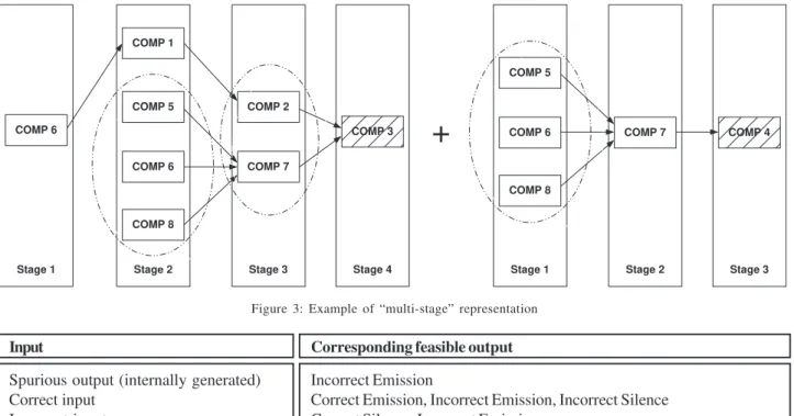
It is a system with eight different components, two of which are root nodes. The corresponding representa-tion, by grouping components in stages, is shown in Figure 3. The original system has been decomposed in two sub-systems of four and three stages, respectively, obtained following the reversal path from each root node to the leaves. We note that COMP 6 is replicated twice in the first

sub-system, as it is originally connected to two different com-ponents (COMP 1 and COMP 7, see Figure 2). We identify the

groups composed of more that one component with a dot-ted circle.

In the following Subsection we detail the system’s behavior, specifying how two generic components may in-teract each other.

2.1 INTERACTIONSBETWEENCOMPONENTS AND MEASURESOFINTEREST

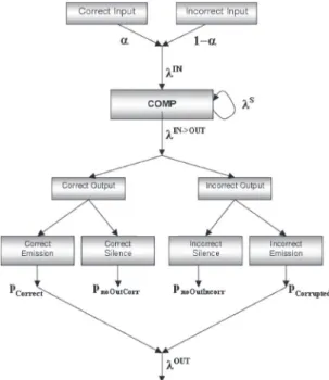
The interactions among components and the failure assumptions on each component are highlighted in Figure 4. This scheme is very general and must be specialized for

the particular component under analysis. To explain the generic component’s behavior, let’s suppose it receives an input following a Poisson distribution with a rate

λ

. These inputs are assumed to be correct or incorrect with a prob-ability

α

α

λ

, the component produces an output with a rate p *

λ

, where p is the probability a received input leads the component to produce an output. Moreover, the component is assumed to possibly behave incorrectly by self-generating spurious outputs with a rate

λ

. Thus, the “potential”1 _{output rate of the component is}

expressed as

λ

₌

λ

₊

λ

For the sake of clarity, we give some deffinitions that we will use in the rest of the paper. A correct emission is the emission of a correct output, that occurs whenever a correct output is produced. It is possible i) in response to a correct input if the system is free from errors, or ii) in re-sponse to a correct input, if system errors are detected and tolerated. A correct silence is the non-emission of an rect output and it may happen as consequence of an incor-rect input (if the incorincor-rectness of the input is detected, for example using interface checks) or of an erroneous status of the system. An incorrect emission is the emission of an incorrect output and it happens either in reply to an incor-rect input, or as consequence of a spurious output or of a wrong processing of a correct input. Finally, an incorrect silence is the non-emission of a correct output and it may happen as consequence of wrong processing of a correct input. These input-output combinations are summarized in Table 1.

COMP 1

COMP 6 COMP 7 COMP 8

COMP 2

; COMP 3

COMP 5

; COMP 4

Stage 2 Stage 3 Stage 4 Stage 1 Stage 2 Stage 3

Stage 1 COMP 6

COMP 1

COMP 5

COMP 6

COMP 8

COMP 2

COMP 7

;; COMP 3

COMP 5

COMP 6

COMP 8

COMP 7

; COMP 4

+

Figure 3: Example of “multi-stage” representation

Input

Spurious output (internally generated) Correct input

Incorrect input

Corresponding feasible output

Incorrect Emission

Correct Emission, Incorrect Emission, Incorrect Silence Correct Silence, Incorrect Emission

Table 1 - Input-output combinations

Therefore, each component can be characterized by two input parameters (

α

λ

) and by the following five output parameters:

- PCorrect, that is the probability of generating acorrect output (correct emission);

- PCorrupted, that is the probability of generating an incorrect output (incorrect emission);

- PnoOutCorr, that is the probability that the output is correctly non-emitted (correct silence);

- PnoOutIncorr, that is the probability that the output is incorrectly non-emitted (incorrect silence); -

λ

, that is the rate of the propagation of an output from the component to another. In particular,

λ

₌

(

λ

.

From the point of view of propagation, it is clear that not all the outputs generated at a stage are always propa-gated up to the root. In fact when a component receives an output (correct or incorrect), it can operate in two different ways, depending on the correctness of the output received and on its internal state: it can generate another output and propagate it to the next stage (emission behavior), or it can not emit any output, thus interrupting the propagation flow (silence behavior).

Given the behavior structure and failure semantics depicted in Figure 4, typical measures of interest from the dependability point of view in this context include:

1. The probability of correct and incorrect emission; 2. The probability of correct and incorrect silence; 3. The overall probability that the system does not

un-dertake wrong actions;

4. The mean time to incorrect emission.

In Section 5 we will specify the measures to evaluate with reference to a particular resource management system.

3 D

The modeling methodology, originally introduced in [2], is fully described in this section. First, we deal with the model design process, that is, how to model a complex system starting from its functional specification and apply-ing a stepwise refinement to decompose it in small sub-models. Then, the second part of the methodology is pre-sented, which concerns the modular model solution, car-ried out in a bottom-up fashion. The philosophy of our modeling approach is shown in Figure 5.

Figure 5: Modeling approach

In order to construct an efficient, scalable and easily maintainable architectural model, we introduce a stepwise modeling refinement approach, both for the model design process and for the model solution. Another advantage of this approach is to allow models refinement as soon as sys-tem implementation details are known or/and need to be added or investigated.

3.1 THEMODELDESIGNPROCESS

The model design process adopts a top-down ap-proach, moving from the entire system description to the definition of the detailed sub-models, while the model solu-tion process follows a bottom-up approach.

As inspired by [3], the system is firstly analyzed from a functional point of view (functional analysis), in or-der to identify its critical system functions with respect to the validation objectives. Each of these functions corre-sponds to a critical service provided by a component.

The overall system is then decomposed in subcom-ponents, each one performing a critical subfunction, and each subfunction is implemented using a model that de-scribes its behavior. Therefore, starting from the high-level abstract model, we perform a decomposition in more elemen-tary (but more detailed) sub-models, until the required level of detail is obtained.

The definition of the functional (abstract) model rep-resents the first step of our modeling approach. The rules and the interfaces for merging them in the architectural de-pendability model are also identified in this phase. The

ond step consists in detailing each service in terms of its software and hardware components in a detailed ( struc-tural) model accounting for their behavior (with respect to the occurrence of faults). The fundamental property of a functional model is to take into account all the relationships among services: a service can depend directly from the state of another service or, indirectly, on the output generated from another service. The detailed model defines the struc-tural dependencies (when existing) among the internal sub-components: the state of a sub-component can depend from the state (failed or healthy) of another sub-component.

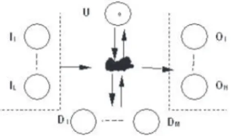
Figure 6: Functional-level model related to a single Service

Figure 6 shows the functional-level model related to a single service. The internal state S is here composed of the place U, representing the nominal state, and of the places D₁ ... D_M, representing different possible erroneous (de-graded) states. The places I₁ ... I_L and O₁ ... O_N represent, respectively, the input (correct or exceptional, due to propa-gation of failures from interacting modules) and the output of the model (correct behavior or failure - distinguishing several failure modes). The state changes (from the nomi-nal, correct state to the erroneous states and viceversa) and the flow between the input and output places are regu-lated by a structural model of the service implementation, indicated in Figure 6 as a black cloud.

3.2 THEMODELSOLUTIONPROCESS

The model solution follows a bottom-up approach from the detailed model up to the abstract model. The imple-mentation is strictly related to the environment characteris-tics of the system under analysis. Actually, starting from the general class of systems of Figure 1, we can derive several simplified systems that can be solved very efficiently.

3.2.1 ENVIRONMENTCHARACTERISTICS

Suppose, for the sake of simplicity, that the generic system of Figure 1 has one root node only. If it is not the case, we can decompose the system in more sub-systems having one root each, as explained in Section 2. We denote with,

λ

the intensity of the output process of the i-th component belonging to stage k ( ). We make the following assumptions:

1. The distribution of the input process of each compo-nent is Poisson with rate,

λ

. This is accepted in the literature when the number of arrivals in a given time interval are independent of past arrivals.

2. The distribution of the output process of each com-ponent is Poisson distributed with a rate,

λ

. This assumption corresponds, for example, to the case in which the inputs are processed sequentially with-out queuing and losses, and the processing time of the input is deterministic. Equivalently, we could obtain the same output distribution considering that the service time is Poisson distributed and that the component operates as a steady-state M/M/1 queu-ing network [4].

Suppose to have a group of components at stage k ( , ..., ). We remind that a group is a set of components belonging to a stage, and connected to the same component in the next stage. Using the assumption that the output process of is Poisson distributed with rate

λ

λ

λ

is equivalent to a Poisson process with intensity equal to

λ + . . . + λ

Solving the detailed model of components COMP%, ... , COMPk leads to the evaluation of the probabilities of correct/incorrect output (both propagated and not propa-gated to the next stage) and the intensity of the output process of a group of components. Let’s defining as

d , and the probability of correct emission, and the probability of incorrect emission of

COMPKI, respectively. Notice that these probabilities de-pend upon the intensity of the input process (

λ

λ

where is the intensity of the process achieved by aggregating the output processes of the

com-ponents , while is the

probability that the next component at stage k + 1 receives a correct input. Analogous considerations hold for , and so on. This general approach can be speci-fied for the following cases:

(II) If all groups at stage k can not be considered identi-cal at each stage, the number of models to be solved depends on the number of diffeerent “branches” in which the overall model can be simplified.

(III) If for each stage k of the system, all the compo-nents are identical, it is possible to solve only K detailed models, one for each stage. Therefore, if all the components at level k are identical, then

the previous equations reduce to

where is the total number of components at stage k.

In this case, the general model of Figure 1 is reduced to the equivalent simplified system model of Figure 7 that can be solved more easily, as the “tree” structure collapses in a unique “branch” from the point of view of system evalu-ation.

We note that case (II) is the more general one; next is case (I) and the least general is case (III). If it can not be assumed that the output process of follows a Poisson distribution, the general approach is still valid pro-vided that the detailed model is slightly modified allowing to estimate the real distribution of such a process. The same distribution will be used as input at the k + 1 stage. How-ever, in general, it will be no longer possible to solve the models analytically.

If the measures of interest are probabilities, the mo-ments of the distribution of correct/incorrect output (both propagated and not propagated to the next stage) which yield such probabilities are not considered at all. In this case it is not necessary to use, at the abstract level, models having the same distribution estimated at the detailed ones. If, on the contrary, we are interested in evaluating the mo-ments, the output processes distributions achieved by the detailed models have to be used for the solution of the abstract models.

3.2.2 THEMODELSOLUTIONSCHEME

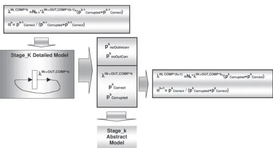
According to Figure 5 (showing the philosophy of our modeling approach) the model solution follows a bot-tom-up approach: the solution of a detailed model is ex-ploited to set up the parameters of the corresponding ab-stract model and of the detailed model of the next (contigu-ous) components (the output of the detailed model acts as input for the detailed model). To keep the

presentation simple, the model solution scheme is described in the case where, for each stage k, all the components at stage k are identical; therefore only K detailed models (one for each stage) have to be solved. Figure 8 shows the rela-tionships among a detailed model of and the model

.

With reference to the measures of interest listed in Section 2.1, the outcomes of the detailed model are:

1. : is the probability that no output is

pro-duced by component , as a consequence of an incorrect input;

2. : is the probability that an expected output is incorrectly not propagated by component

, as consequence of an internal fault;

3. : is the rate

of messages propagated by component to

component ;

4. : is the correct emission probability;

5. : is the emission failure probability. This value encompasses both an expected wrong emis-sion (as consequence of wrong internal processing) and the unexpected emission (as consequence of an internal self-generated false alarm).

All these parameters are used in the abstract model of component (see Figure 8) while are used to derive the parameter to be used in the detailed model of . In the system framework and

represent two components directly connected that exchange messages in one direction (from to ).

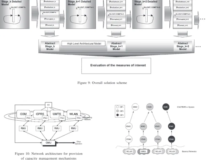
Summarizing, the overall solution scheme is shown in Figure 9. The detailed models are solved separately: firstly the model of is solved, then the values provided by equations (3) and (4) are passed as input to the detailed model of and so on. Finally, the probabilities of correct/incorrect output (both propagated and not propa-gated to the next stage) are passed to the corresponding abstract models, they are joined together and then the overall abstract model is solved.

respect to the measures of interest, is achieved by joining the abstract models.

4 A

“

-

”

:

CAUTION++

The IST-2001-38229 CAUTION++ project [1] aims at developing a novel, low cost, flexible, highly efficient and scalable system able to be utilized by mobile telephone op-erators to increase the performance of all network segments. Capacity utilization in cellular networks is an extremely im-portant issue from the operators’ point of view. Successful usage of all the system resources especially in congestion situations can imply increased revenues for the cellular net-work operators via reduced call blocking and dropping rates. Also, in emergency situations the cellular networks are

ex-pected to work properly and be able to respond to the mo-mentarily increased offered trafic. To pursue such goals, proper system components are developed to handle gener-ated alarms through a set of RRM (Radio Resource Man-agement) techniques, to be applied where needed. The CAUTION++ system, superimposed over the existing wire-less networks, should allow putting in place correctly the identified RRM techniques, hopefully despite the occur-rence of faults. The rationale is to enforce design solutions able to prevent a CAUTION++ component from carrying out a reconfiguration action wrongly or when it is not nec-essary (as consequence of some fault). Because of the in-volved functionalities which pose relevant dependability issues, the CAUTION++ project has promoted model-based evaluation, aiming at assessing dependability attributes of the architecture under development.

Figure 7: Part of the simplified system model

Figure 10: Network architecture for provision of capacity management mechanisms

Figure 10 shows the main components of the CAU-TION++ architecture. Each network segment has its own ITMU (Interface Trafic Monitoring Unit) and RMU (Re-source Management unit) which allow to monitor and man-age the attached network, respectively. Within each opera-tor network, a GMU (Global Management unit) can perform a global optimization. A Location Server (LS) can be used to track users’ mobility and location: such information can be exploited by GMU for a global optimization.

To practically show the usage of the proposed mod-eling methodology, in this paper we consider a specific architecture’s instance involving GSM/GPRS and WLAN network technologies deployed by two distinct operators, which is actually one of the trial systems set up by the consortium as a demonstrator of the project’s results.

From the point of view of system composition, Fig-ure 11 depicts the components included in such trial. Three operators are involved, Op1, Op2 and Op3, with Op1 and Op3 managing a WLAN network only, and Op2 managing both a GPRS and a WLAN network. From the point of view of CAUTION++ components employed in this instance, each network segment has its own ITMU (Interface Trafic Monitoring Unit) and RMU (Resource Management Unit)

which allow to monitor and manage the attached network, respectively. Within each operator network, a GMU (Global Management Unit) is necessary to perform a global optimi-zation. In fact, different GMUs cooperate to optimize among different operators. Therefore, this CAUTION++ instance includes 4 ITMU, 4 RMU and 3 GMU, connected as shown in Figure 11.

It is clearly an instance of a multi-stage system. Start-ing from the GMU components (the root nodes of the graph, see Section 2), we decompose the system in three sub-systems, one for each GMU. Each subsystem can be seen as a “3-stage” system, that is a “multistage” system com-posed of 3 stages, in which all the components belonging to a stage are identical. Moreover, each subsystem can be represented as shown in Figure 7, as the “tree” structure collapses in a unique “branch” from the point of view of system evaluation. Therefore we have to solve only 3 de-tailed models for subsystem.

4.1 COMPONENTSBEHAVIORAND MODELINGASSUMPTIONS In order to set up the detailed models, a character-ization of the system components from the dependability point of view is necessary, briefly outlined in the following.

Figure 9: Overall solution scheme

- Each CAUTION++ element (ITMU, RMU, GMU) can be either correctly working or wrongly working.

- Each CAUTION++ element (ITMU, RMU, GMU) is composed by three main elements: the Application Soft-ware (AS), the Operating System (OS), and the Hard-ware (HW). Each element has its own dependability figures and reference values, that have been chosen as explained later. In turn, the AS, OS, and HW can be either correctly working or wrongly working.

- At the end of its computation, each CAUTION++ component can emit an output or not. More pre-cisely, the possible output can be either correct/in-correct emission or correct/in-correct/incorrect/in-correct silence.

- Fault tolerance mechanisms are in place in each sys-tem component, in order to improve the dependabil-ity of the components themselves and limit the error propagation between interacting elements. They are interface checks (to detect errors at input/output level), diagnosis and repair mechanisms. Their abil-ity to work properly depends on their respective coverage.

In addition, a set of assumptions has been identified with the aim of enhancing simplicity and clarity (essential to keep the whole modeling activity under control), still capturing the relevant phenomena which impact the mea-sures under analysis (essential to the practical usefulness of the evaluation effort). The complete list is in [5] and [6]; here we omit those strictly related with details of the models not shown in this paper.

- The input to the detailed model may be either correct with probability

α

α

- Each CAUTION++ element (ITMU, RMU, GMU) can generate by itself spurious outputs (that is, outputs not triggered by an external input; it is a manifesta-tion of a fault in the component). Spurious outputs are independent from outputs generated by real in-puts and follow an exponential distribution.

- The coverage of the Input interface checks is given by the probability inputCoverage. When Output in-terface checks are considered, the detection of an erroneous output leads to a non-emission of an out-put (silence behavior, which may be correct or incor-rect depending on the inputs originating it and/or on the correctness of the component’s status) with probability outputCoverage.

- An undetected erroneous state of the AS may disap-pear when the OS is repaired, e.g. in the case of OS re-booting.

- An undetected erroneous state either at the AS or OS level may disappear when the HW is repaired (because of necessary system reboot, no hot-pluggable redundancy is envisioned).

- An undetected erroneous state either disappears or propagates and reveals itself.

5 S

CAUTION++

In this Section, the models derived for the analysis of the selected CAUTION++ instance of Figure 11 are briefly outlined. First, the measures of interest are described, since they influence the definition of the system models.

5.1 MEASURESOFINTEREST

As previously mentioned, the goal of the CAU-TION++ system is to increase the performance of all the controlled cellular networks. Then we expect it should never have a negative impact on the networks behavior, at the most becoming inactive in the worst case. Therefore, the main dependability requirement of CAUTION++ is that it should avoid taking wrong decisions, thus acting worse than doing nothing.

Particularly, an incorrect silence behavior (that is the system does not provide any output when, if correct, it would have emitted one) can be tolerated, since it leads to no benefit from CAUTION++. On the contrary, an incorrect emission of an output can lead the system to act worse than doing nothing, and therefore actions would be required to prevent such failure mode.

We have identified the following indicators as sig-nificant measures to evaluate the dependability of the CAU-TION++ architecture. They are:

- The probability of incorrect emission at level of the GMU employed by a certain operator;

- Mean Time to Failure of the GMU employed by a certain operator;

- Reliability of the whole system(with contributions from all the present GMUs).

They appear to be suitable measures to evaluate the ability of CAUTION++ in fulfilling the general dependabil-ity requirement of not undertaking wrong reconfiguration actions.

5.2 DETAILEDAND ABSTRACTMODELS

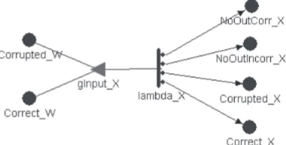
In accordance with the proposed methodology de-scribed in Section 3, the starting point is the definition of a functional model for each involved component. Each func-tional (“abstract”) model has to take into account all the relationships among critical services that, in this trial, are the emissions of outputs from ITMU to RMU and from RMU to GMU. The generic “abstract” model is represented in Figure 12, using the SAN [7] formalism.

It is valid for ITMU, RMU and GMU. The input gate gInput_X allows handling the input of the component (both the correct input - place Correct_W and corrupted input -place Corrupted_W). Transition lambda_X fires with a rate,

where, are the

rate of messages in input to component X and the rate of spurious messages generated by X, respectively.

Then, an output is produced. This output can be either correctly emitted (a token is moved in place Correct_X with probability pCorrect_X) or incorrectly emitted (a to-ken is moved in place Corrupted_X with probability pCorrupted_X) or correctly non-emitted (a token is moved in place NoOutCorr_X with a probability pnoOutCorr_X) or incorrectly non-emitted (a token is moved in place NoOutIncorr_X with probability pnoOutIncorr_X). An out-put is propagated at the upper level of the CAUTION++ hierarchy (or as final output in case of GMU) with a rate .

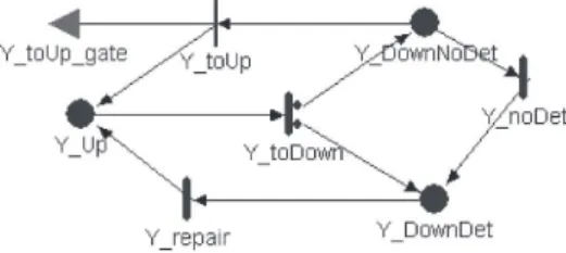
To obtain the parameters of each abstract model, the corresponding detailed models have to be set-up and solved. Therefore, a detailed model is built for each involved com-ponent. Since ITMU, RMU and GMU employ the same sub-components (HW, OS and AS, plus fault tolerance mecha-nisms, as already discussed), the detailed model is almost the same for all of them. The only difference is in the values of their parameters (as explained later in the section on nu-merical evaluation). A generic detailed model is obtained by composing the generic detailed models for the component’s subcomponents (i.e., HW, OS and AS) together with the dynamics of the error and fault detection mechanisms em-ployed. The presentation of this model is omitted for brev-ity (refer [5] for a complete exposition); here only a simpli-fied generic detailed model for the subcomponent Y (where Y maybe AS, OS or HW) is sketched in Figure 13.

Figure 13: Detailed model for AS, OS, and HW

A token in place Y_Up indicates that Y is working correctly. The firing of transition Y_toDown models its fail-ure: this failure can be detected (a token moves in the place Y_DownDet) or not (a token moves in the place Y_DownNoDet) with probabilities Y_Coverage and 1-Y_Coverage, respectively (Y_Coverage represents the coverage of the error detection mechanisms implemented in the element Y). An undetected failure can be revealed after a while; the firing of transition Y_noDet indicates such fail-ure detection. A detected failfail-ure is then recovered by means of the transition Y_repair. An undetected erroneous state

may disappear if the input gate Y_toUp_gate enables the instantaneous transition Y_toUp, for example in the case of OS re-booting if Y = AS.

The overall model for the CAUTION++ instance under analysis has been constructed under the following assumptions:

- Messages coming from different ITMUs and RMUs are indistinguishable.

- The RMUs and the GMUs process the incoming input requests (from the ITMUs and RMUs respec-tively) individually and sequentially.

Figure 14: Composed model at GMU decision level

Figure 14 shows the SAN composed model for ana-lyzing the CAUTION++ behavior at a single GMU decision level (e.g., to evaluate the probability of correctness of a reconfiguration decision issued by a GMU). Thanks to the above assumptions, the evaluation of the whole CAU-TION++ instance is easily obtained by mathematically com-bining the evaluations at single GMU level, in accordance with the specific measure under analysis.

6 E

The preceding models have been numerically solved using the analytical solver provided by the Möbius tool [8]. Since all the timed transitions are exponentially distributed and the state space dimension of the models was not huge, it was possible to pursue an analytical solution achieving more accurate results than through simulation. Given the nature of the measures of interest, we resorted to a steady-state analysis for all models.

6.1 SETTINGSFORTHENUMERICALEVALUATION

substi-tuted by ITMU, RMU, GMU to indicate the parameters of the corresponding component. Since the models have been just sketched in this paper, not all the involved parameters have been listed in Table 2.

The values assigned to the missing parameters are the same applied in [5].

Table 2: Varying model parameters and Their values

The meaning of the parameters in Table 2 is as fol-lows:

-

α

α

α

the input provided to ITMU, RMU and GMU, re-spectively, is correct;

- MTBA_ITMU, MTBA_RMU and MTBA_GMU are the mean time between two inputs to ITMU, RMU and GMU, respectively (in the case of ITMU, it is the mean time between two external inputs for which ITMU generates an alarm to RMU);

- MTBFA_X is the mean time between two spurious outputs emitted by a generic component X ;

- InputCoverage_X is the coverage of the error detec-tion checks at input interface;

- OutputCoverage_X is the coverage of the error de-tection checks at output interface;

- AS_Coverage_X is the coverage of the application software checks.

6.2 NUMERICALEVALUATION

In this section, we present and discuss the results obtained. To keep the notation in the figures as light as possible, we indicate with I/OCov the coverage of the input and output interface (which is the same for ITMU, RMU and GMU), and with ASCov the coverage of the application software (again, it is the same for ITMU, RMU and GMU).

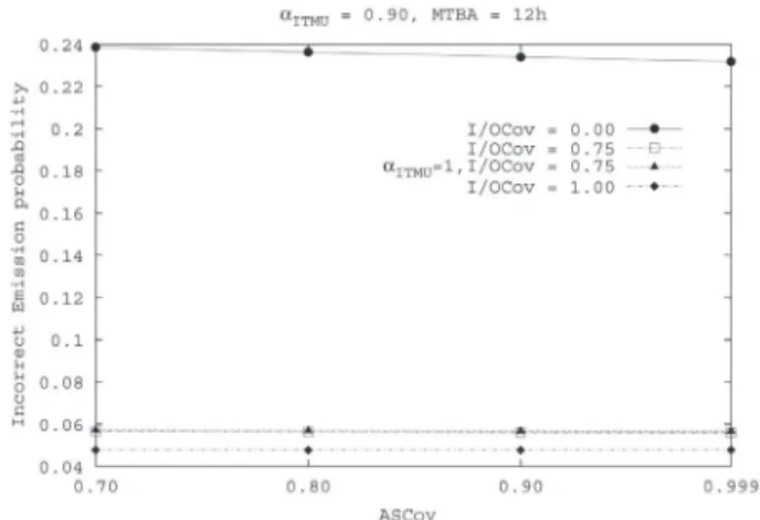
Figure 15 shows the probability of incorrect emis-sion of the GMU managed by Operator1 (it is actually the same for Operator3 also), at varying values of the coverage of the I/O Interface Checks and the coverage of the Appli-cation Software. The probability of incorrect emission de-creases as the probability of coverage of the I/O Interface

Checks increases; instead, it is very lightly influenced by As Coverage. Looking at the two overlapping curves, it can be observed that the impact of the correctness of the input to ITMU is not relevant. Therefore concerning the emis-sion failure probability, significant benefits are achieved using the Interface Checks, since more incorrect messages are detected and no output is produced in these cases.

Figure 16 shows the reliability of the trial system at varying the observation time, that is the overall probability that the system does not undertake wrong actions. We sup-pose that the overall system fails if at least one root compo-nent fails or, equivalently, one GMU undertake a wrong action. The reliability of the trial system at time t is then equal to e

and is the mean time to failure related to operator i. Therefore, we have solved the three operators sub-nets separately, and then we have obtained the reliability for the whole system by exploiting the previous formula.

The plots have been obtained by fixing the mean time between alarms to 12 hours and the probability of cor-rect input to ITMU to 0.98. The varying parameter is the MTBFA. The reliability of the system quickly decreases at

Figure 15: Incorrect emission probability related to Operator 1 (or Operator 3)

lower values of MTBFA. In the figure, also an “extreme case” curve is plotted, obtained considering totally correct the external input to the ITMU, and assuming a very high coverage (0.99) for all the employed error detection mecha-nisms. The idea was to understand how would be the reli-ability of the CAUTION++ instance, in case a highly robust implementation of the CAUTION++ components is per-formed and in absence of faults external to the system. It can be appreciated that in such a case the reliability curve has a very good trend.

Despite the insertion of CAUTION++ induces a small reliability penalty (as exemplified by Figure 16), it is never-theless very beneficial, since CAUTION++ allows to in-crease the resource utilization of the underlying networks through a cooperation among them. This is the final goal of the project that justifies the existence of system and the consequently introduction of new errors.

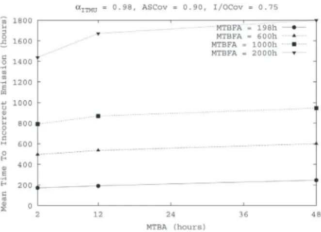
Figure 17 and Figure 18 are plotted at varying values of the mean time between alarms and the mean time be-tween spurious outputs, and setting to 0.98 the probability that the input to ITMU is correct. Not surprisingly, all the curves follow an increasing trend. Note that the time to an incorrect emission is significantly different for Operator 1 (or Operator 3) and Operator 2.

7 C

This paper has focused on a methodology for quan-titative dependability evaluation of systems structured in a hierarchical fashion and on its application to a case study.

In more details, in the first part of the work an effi-cient modeling methodology has been presented, consist-ing in definconsist-ing “abstract” and “detailed” models of the sys-tem components, so as to reduce complexity and gain effi-ciency both at model design and at model solution levels.

In the second part, an instance of the CAUTION++ architecture has been selected, as a representative case study of the class of systems our methodology is directed to. In accordance with the basic dependability requirements stated in CAUTION++, the evaluated dependability indica-tors have been the probability of an incorrect output emis-sion, the Mean Time to Failure of a GMU component and the reliability of the whole instance. We resorted to an ana-lytical solution, using the automatic Möbius tool.

Thanks to the application of our modeling method-ology and resolution technique, the biggest model solved had less than 1000 states, and the time needed to perform a single study did never exceed one minute on a Pentium M 1.3 GHz, 512Mb Ram PC. Actually, most of the time required to the resolution technique is due to the manual passing of the parameters’ values between the detailed models and from these to the abstract one. Such waste of time could be significantly reduced using an automatic tools that could be developed in future works. The same simple trial could hardly be solved just considering a monolithic model com-posed of three detailed submodels only. In fact, supposing an average of 500 states per submodel, the size of the state-space would be of the order of magnitude of 108

(500x500x500). Although this is only an approximated cal-culus that, in addition, does not take into account the pos-sible symmetries that could reduce the size of the overall state-space, it lets us appreciate the contribution of the proposed methodology in solving such types of systems.

Of course, there is still work to do in evaluating the effectiveness of the methodology in more complex sce-narios. Anyway, the indications that we are able to provide at the moment, as derived from this study, seem to be very encouraging.

The obtained results allow to understand the impact of several factors contributing to the dependability of the single CAUTION++ components on the overall system in-stance. Moreover, this study can be useful to guide imple-mentation choices addressing dependability, by providing comparative quantitative assessment of possible alternatives.

A

This work has been partially supported by the Euro-pean Community through the IST-2001-38229 CAUTION++ project and by the Italian Ministry for University, Science and Technology Research (MURST), project “Strumenti, Ambienti e Applicazioni Innovative per la Societa’

Figure 17: Mean time to incorrect emission for Operator 1 (or Operator 3)

dell’Informazione, SOTTO-PROGETTO 4”. The authors want also to acknowledge the contribution given by Stefano Porcarelli to the early phases of this work.

R

[1] CAUTION++ IST Project. Capacity Utilization in Cellular Networks of Present and Future Genera-tion++. http://www.telecom.ece.ntua.gr/ CautionPlus/.

[2] S. Porcarelli, F. Di Giandomenico, P. Lollini, and A. Bondavalli. A modular approach for model based dependability evaluation of a class of systems. In International Service Availability Symposium (ISAS 2004), Lecture Notes in Computer Science, Springer-Verlag, volume 3335, pp.160-174,2005. [3] C. Betous-Almeida, and K. Kanoun. Stepwise

con-struction and refinement of dependability mod-els. In Proc. IEEE International Conference on Dependable Systems and Networks DSN 2082, Washington D.C., 2002.

[4] K. S. Trivedi. Probability and Statistics with Reli-ability, Queuing, and Computer Science Applica-tions. John Wiley and Sons, New York, 2001. [5] S. Porcarelli, F. Di Giandomenico, A. Bondavalli,

and P. Lollini. Model-based evaluation of a radio resource management system for wireless net-works. In Computing Frontiers (CF), pages 51-59, Ischia, Italy, April 2004.

[6] CAUTION++ IST Project. D-3.6: Report of model-based validation activities.

[7] W. H. Sanders, and J. F. Meyer. A Unified Ap-proach for Specifying Measures of Performance, Dependability and Performability. In Dependable Computing for Critical Applications, volume 4 of Dependable Computing and Fault-Tolerant Sys-tems, pages 215-237. Springer-Verlag, 1991. [8] D. Daly, D. D. Deavours, J. M. Doyle, P. G. Webster,

and W. H. Sanders. Möbius: An Extensible Tool for Performance and Dependability Modeling. In 11th International Conference, TOOLS 2000, vol-ume Lecture Notes in Computer Science, pages 332-336, Schaumnurg, IL, 2500. B. R. Haverkort, H. C. Bohnenkamp, and C. U. Smith (Eds.). [9] M. Balakrishnan and K.S. Trivedi. Component wise

decomposition for an efficient reliability compu-tation of systems with repairable components. In Int. IEEE Symp. Fault-Tolerant Computing (FTCS-25), pages 259-268, 1995.

[10] G. Balbo, S.C. Bruell, and S. Ghanta. Combining queuing networks and generalized stochastic Petri nets for the solution of complex models of system behavior. IEEE Trans. Computers, 37(10):1251-1268, 1988.

[11] I. Mura and A. Bondavalli. Hierarchical modelling and evaluation of phased-mission systems. IEEE Transactions on Reliability, 48(4):360-368, 1999. [12] I. Rojas. Compositional construction of SWN