doi: 10.1590/S0103-65132011005000069
*USP, São Paulo, SP, Brasil Recebido 17/06/2009; Aceito 02/12/2010
Hedging in the ethanol and sugar production:
integrating financial and production decisions
Anna Andrea Kajdacsy Balla Sosnoskia, Celma de Oliveira Ribeirob*
a[email protected], PETROBRÁS, Brasil b*[email protected], USP, Brasil
Abstract
Agricultural producers face financial risk at the moment of final products selling. This imposes the use of instruments to reduce risks in order to assure prices and production process economic feasibility. This paper examines the problem of creating hedging strategies with production constraints and proposes a deterministic multi-period optimization model to solve it. Uncertainty was introduced in the model through scenario trees and risk was analyzed according to the traditional mean variance approach. The model was analyzed for the sugar and ethanol market in order to aid in the financial management of a sugar cane refinery.
Keywords
Optimization. Hedging. Agricultural commodities. Sugar and ethanol sector. Risk.
1. Introduction
The development of domestic sugarcane agribusiness and the uncertainty in products prices requires complex financial and production strategies from producers. The sugar and the alcohol markets are characterized by great uncertainty and producers must adopt adequate production and financial restructuring policies.
The use of buy and sell strategies in the derivatives market is usual, especially on the futures market. Futures markets are liquid and appropriate to fix future prices of commodities and to reduce financial risks. There is extensive literature on risk reduction strategies in the futures market. Usually it is assumed that investors own (or should buy) an asset and try to sell (or buy) the same asset in the futures market in order to fix the future price. In general, asset management is not considered and production decisions are taken without considering the financial strategy. In order to fill the gap between financial risk reduction and production management, this article presents hedging strategies in futures markets considering the production decisions in a sugar & alcohol plant.
There are different risks related to production and sales of products derived from sugarcane. This article deals with price risk management. Price risk consists in the possibility of the final product price moving against the producer’s interest, falling to levels below the production costs. In the case of the sugar & alcohol markets, pricing is a complex task not only from the forecasting point of view, but also regarding the stochastic processes that describes prices - what hinders the construction of strategies.
The article is organized as follows. Section 2 presents concepts related to prices of commodities and hedging strategies. The proposed model is presented in section 3. Computational results are discussed in section 4 and the conclusion is presented in section 5.
2. Price risk and hedging in the sugar
&
alcohol market
protectionist policies among other factors. Commodity prices present high volatility, what significantly hinders the financial management by the industry agents. There are two important questions for rural producers to answer: how to finance the production from planting to harvest, and how to fix prices at the end of the harvest. To finance production, the producer can count on several alternatives which include different credit securities ruled by law. Commodities can be traded in different markets: the spot market, forward market, or through anticipated sale contracts, which include the futures markets.
Seasonal movements resulting from planting and harvest conditions, the worldwide market characterized by protectionist barriers and government interference hamper the decision making. Sugarcane harvest begins in the autumn and it determines the price behavior of the products. During the rain season in Brazil (September to March), sugarcane production falls, rising again between April and August - period of little rainfall. Technological evolution in cultivation and production process of sugarcane and its by-products changed the season and off season periods. As a result it is not possible to identify seasonality in prices through statistical analysis. In the case of sugar, prices movements are observed due to supply-demand imbalance at worldwide level.
There are several instruments in the derivatives market to reduce price risk, especially the futures and options markets. This article deals specifically with the strategies that use the futures market. Combining spot and futures market positions, it is possible to reduce the price risk to which a producer is exposed. These operations are known as hedging strategies. Hedging strategies in future markets have been studied for over five decades. Working (1953), in a classic article about commodities hedging, discusses the role of futures markets as a protection instrument against price fluctuation. The author deals with the use of strategies with futures by the various market agents, highlighting the fact that farmers did not use these tools. Collins (1997) features the wide range in the use of hedging strategies, which are dependent on the agents who make use of them in the supply chain, and stresses the importance of investment funds within this market. Tomek and Peterson (2001) discuss the approaches used by agricultural producers in price risk management and point out the difficulties in the construction of models for the elaboration of hedging strategies. Garcia and Leuthold (2004) show - as an important research area - the connection between hedging and the producer’s capital structure.
Usually hedging strategies refer to constructing a portfolio which maximizes the expected utility of the investor or minimizes some risk measure. That
is, one seeks to solve the problem maxCf E [U(Cf )], where Cf is the amount of future market contracts that shall be bought (or sold) for each unit of spot asset Cs available. The function U(.) represents the investor’s utility. It is assumed that the cash position is fixed, and an optimal position in the future is sought, with the utility function reflecting the investor’s risk aversion. The quotient f
s C
C is named hedge ratio (delta).
There are two approaches to construct hedging strategies: the static, which supposes that the hedge ratio remains constant over time, from the moment the strategy is created until the time one position is reverted (at the maturity of the future contract or at the execution of the spot position); and the dynamic, that changes over time and calculates the hedge ratio based on conditional information (CHEN; LEE; SHRESTHA, 2003). A well-known static model is the minimum variance hedging ratio, proposed by Johnson (1960), where the portfolio risk is minimized. The risk is measured through the variance of value changes in the hedged portfolio, and it leads to a simple expression for the calculus of the hedge ratio. In this article an approach consistent with the models of portfolio selection proposed by Markowitz (LUENBERGER, 1997) is used.
Few articles in the literature deal with portfolios including real and financial assets. Chen, Lee and Shrestha (2003) analyze multi-period models for pricing and inventory policies management, based on additive utility measures which incorporate aversion to the investor’s risk. Geman and Ohana (2008) analyze holding and selling of contracts by a retailer under stochastic demand and price
3. The model
{
}
1
1 2
t t t t t
X V VF A A
t , , ,H
−
= + + −
∈ (1)
The model maximizes the expected utility of the investor by the end of one-year period (in working days). There are H decision moments in one year, which match the maturity dates in the futures market (in the case of the Brazilian market, H = 5, corresponding to February, April, July, September and November). The constraints of the productive system refer to the production capacity, the maximum capacity for sugarcane processing and the availability of raw material in each period of the year (it is not possible to store sugarcane for processing in a coming period). The minimum demand of the market for sugar and alcohol must be met within upper and lower production limits. Due to capacity limits to the physical storage of sugarcane by products, it is necessary to assure inventory turnover, avoiding excessive inventory. It is noteworthy that the production share allocated for sale in the futures market needs to remain stored until the next maturity date. The model does allow to sell more than 100% of the production in the futures market.
The production of second quality alcohol from the bagasse resulting of the original production and the opportunity of generating energy from this bagasse might be considered. If production and storage costs are known, as well as the return obtained with the trading of these by-products, the model could decide what to do with the bagasse. However, there is no data available for analysis of these variables and they were not included in the model. The uncertainty in the model results from changes in sugar and alcohol prices, described by the scenarios tree. The costs and the demand are deterministic and it is assumed that the plant owner limits hedging to a maximum percentage of production.
3.1.
Parameters
• I = {1,..., N}: indexing of products that can be produced by the plant.
• T = {1,2,..., H}: indexing of time periods. • Γ = {1,2,..., S}: indexing of scenarios.
• πs s ∈Γ: probability of occurrence of scenario s. • Cei: cost of storage and manufacturing of product i. • Cpis: production cost of product i in scenario s. • PFis (t ): price of first maturity future contract of
product i, at time t, at scenario s.
• Pis (t ): price of the product i ∈ I, at the time t, at scenario s.
• Di (t ): demand of product i, at time t.
• Cestoque,i (t ): storage capacity of product i, at time t. • C (t ): amount of sugarcane available at t time.
Maximum amount will be equal to 1 (100% of production capacity). During off season periods this amount is reduced to 0.
• K: minimum capital required for each period. This value is estimated as the minimum wealth to keep the plant working and to allow business investments. • ConvX→Y: converser to set amount obtained of
product Y from a certain amount of product X
3.2.
Decision variables
For every t ∈ T
• Ai(t ): amount of product i, i ∈ I, stored in time t.
• Vi(t ): amount of product i, i ∈ I, sold in time t.
• VFi(t ): amount of product i, i ∈ I, sold in the future market, decision making in t and liquidation of the position in t + 1.
• CFi(t ): amount of product i, i ∈ I, bought in the future market, decision making in t and liquidation of position in t + 1.
The decision variables are measured in percentage of the plant capacity. This article presents the deterministic version of the model where the decision variables do not depend on the scenario considered, that is, a stochastic optimization approach is not adopted. The uncertainty in prices is described by a scenarios tree, so that the wealth in time t in a scenario s is given by Rs(t ), t ∈ {1,...,H} s ∈ {1,2,...,S}.
3.3.
Constraints
It is assumed that hedging strategies are implemented only in the sugar futures market as there is no alcohol futures market. The following constraints assure basic operation conditions of the plant :
( )
( )
( )
1
1 1
1 1
2
N
s i is cana i i i cana i
i
i i i cana i
is is is i cana i
is is i cana i
R ( t ) ( V ( t )P ( t ) Conv X ( t )Cp ( t ) Conv
VF ( t ) A ( t ) Ce ( t ) Conv
P ( t ) PF ( t ) PF ( t ) VF ( t )Conv PF ( t ) PF ( t ) CF ( t )Conv
t { , ,H } s
→ →
=
→
→ →
=∑ − +
− + +
+ − − − +
− − −
∀ ∈ ∀ ∈ Γ
(2)
1 2
i i i i i
X ( t ) A ( t ) A ( t ) V ( t ) VF ( t )
t { , ,H } i I
= − − + +
∀ ∈ ∀ ∈ (3)
1 N
i
i= X ( t ) C ( t ) t T
= ∀ ∈
∑ (4)
1 2
i i i
D ( t ) V ( t ) VF ( t )
t { , ,H } i I
≤ + −
0
i
A ( t ) ≥ ∀ ∈t T ∀ ∈i I (6)
0
i
X ( t ) ≥ ∀ ∈t T ∀ ∈i I (7)
0
i
VF ( t ) ≥ ∀ ∈t T ∀ ∈i I (8)
0
i
CF ( t ) ≥ ∀ ∈t T ∀ ∈i I (9)
1
i
CF ( t ) ≤ ∀ ∈t T ∀ ∈i I (10)
i estoque , i
A ( t ) C≤ ( t ) ∀ ∈t T ∀ ∈i I (11)
s
R ( t ) K≥ ∀ ∈t T ∀ ∈ Γs (12)
The first constraint (Equation 2) describes the financial results obtained with products sales. Prices refer to units of final products. Conversion factors are considered because variables are described in percentage of sugarcane available. It is worth noting that the restrictions are indexed in scenarios, due to the uncertainty of prices. The model will maximize the expected value of a utility function, as presented later, being necessary to describe the price dynamics.
The second constraint (Equation 3) presents the total availability of the product, in percentage of sugarcane, resulting from inventory changes and the amount produced for future market and spot sales. Constraint (4) indicates that the amount available (in percentage of sugarcane) shall not exceed the total sugarcane available in the period. Demand constraint is presented in (5). The non-negativity of variables is shown in constraints (6), (7), (8) and (9). The purchase in the future market cannot exceed the total amount of sugarcane available, as indicated in constraint (10). Storage capacity is described in constraint (11). Finally, the last constraint refers to the minimum financial result to be met in each scenario, in all time periods.
3.4.
Objective function
Consider vectors Vt = (V1(t ),...,VN(t )), VFt = (VF1(t ),...,VFN(t )), and CFt = (CF1(t ),...,CFN(t )) and ft = [VtVFtCFt]. Two situations will be analyzed: utility measures which consider the result at the end of the planning horizon (i.e. maximize E(U(fH ))) and alternatively, additive measures, E(U(f1, f2,...fH )), where
1 2
1
( , H) H t( )t
t
U f ,f f
U f
=
= ∑
. The wealth and the investor’s
risk are considered, with the risk being measured through the variance of wealth. The importance of the wealth and risk depend on the investor’s risk aversion, so that U(ft ) = R(t ) – η(R(t ) – Ε(R(t )))2. The parameter η indicates the investor’s risk aversion.
4. Model application and results
4.1.
Parameters choice
It is assumed that uncertainty results exclusively from sugar and alcohol prices changes. Demand, costs and other parameters are deterministic, obtained through market information or the producer’s expertise. Data on production costs of alcohol and sugar were gathered by a survey performed by “Embrapa” (Empresa Brasileira de Pesquisa Agropecuária) and “UNICA” (União da Indústria de Cana-de-Açúcar) in September 2006. Closing prices of alcohol and sugar contracts in the spot market were obtained at the “Cepea/Esalq” website from July 7, 2000 to July 7, 2007. The prices of sugar and alcohol in the futures market were obtained from “BM&F Bovespa” (Bolsa de Valores, Mercadorias e Futuros).
The other parameters were determined through scenario analysis. It is assumed that the plant owner will obtain raw material uniformly during harvest and no availability of raw material during off season. Following the preceding notation, it means that during harvesting months the availability is C(t) = 1 (100%) and for the off season months C(t) = 0 (0%). The same procedure was adopted for the determination of the minimum wealth.
The conversion factors: cane to sugar, cane to alcohol, and bagasse to its by-products, were collected by a study performed by “UNICA” to investigate the gains obtained with energy cogeneration. Originally, the model considered other variables such as second quality alcohol and energy generated from bagasse. As the data related to these prices were not reliable these variables were not included in the model.
4.2.
Scenarios tree generation
To describe the behavior of prices, a scenarios tree was built based on Monte Carlo simulation. It is assumed prices are described through a mean reversion stochastic process, the usual approach adopted for describing of agricultural commodities prices (GEMAN; OHANA, 2008; SCHWARTZ, 1997; SCHWARTZ; SMITH, 2000). The price dynamics adopted was similar to Tseng and Barz (2002):
= −µ − + σ
∈
j j j j j j
t t t t
d ln( P ) (ln( P ) m )dt dB
j I
(13)
where dBtj are correlated Wiener’s processes, Ptj are
the prices µj, j t m and j
σ are the parameters of the
model ∀ j ∈ I.
Simulation was based on this model. Parameters
j
µ , j t
m and σj were adjusted based on historical data,
also following the Tseng and Barz (2002) approach. Cholesky factorization was used to generate sugar and alcohol data simultaneously in order to consider the correlation between prices. This model was then used for the simulation of a 249-day horizon corresponding to the number of business days between February 2, 2006 and February 2, 2007. This period corresponds to a complete sugarcane cultivation cycle.
In order to build a scenarios tree for both products simultaneously, a clustering technique was adopted, following Gulpinar, Rustem and Sttergren (2004). Consider S paths generated by Monte Carlo simulation:
(
2 3)
1
( s ) ( s ) ( s ) ( s )
J P ( ),P ( ), ,P ( H ) ,
s { , ,S }
=
∈
(14)
P (s ) (t ) represents the prices vector along path s, in time t, originated from an initial deterministic price vector P(1), common to all paths. For each t, the paths are grouped and two clusters are created using Euclidian distance 1 2 2
2
( q ) ( q )
P ( t ) P− ( t ) as a
measure of dissimilarity. Once the cluster is determined a vector to represent one node of the scenarios tree – the centroid – is chosen. Among well known approaches, the centroid was defined as the mean value of prices from that cluster.
The tree is generated sequentially , with each tree level corresponding to a time period. Level 1 (t = 1) of the tree consists of the initial vector of prices, node
1 1
N . At level 2 (t = 2) two nodes are built – 1 2 N and
2 2
N – from the clusters, each node being identified by its respective centroid. The paths originating from the two clusters are the ones employed in the construction of the tree nodes of other layers. Thus, being M2q the number of paths passing through the
cluster q, of the period (t = 2), the process is repeated
in a similar manner. From node 1 2
N and the 1 2 M paths associated to it, two new clusters are built. The same occurs to node 2
2
N and its correspondent paths. The process is repeated successively at all tree levels until it reaches the leaves (t = H ).
4.3.
Computational results
The constraints on demand and minimum wealth requirement led to an infeasible model. As the main focus is the analysis of financial strategies the demand constraint was relaxed and it was chosen to achieve minimum wealth.
The results obtained through the maximization of wealth (with parameter η = 0) are shown in Table 1. This table presents the percentage of alcohol on spot sale (Valc), the sales and purchases in the alcohol futures market (Vfalc and Cfalc), the stored amount of alcohol (Ealc), the percentage of sugar cash sales (Vsu), the sales and purchases in the sugar futures market (Vfsu and Cfsu), as well as the stored amount of sugar (Esu).
The sum of spot sales, future sales and the inventory changes for both alcohol and sugar from one period to the next shall not exceed 100% in order to obey the constraints. However, as the inventory is cumulative and it may not be used for sales in the next period, its value can exceed 100%. Purchases in the futures market are limited to 100% of the plant capacity, and do not impact the capacity constraints, as it does not mean buying the physical commodity (Table 1).
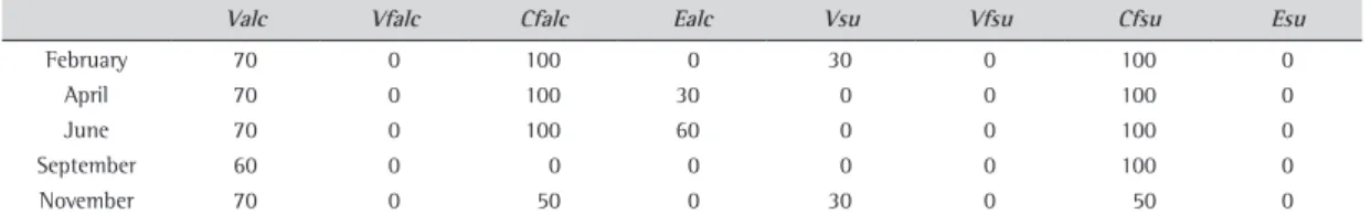
When the sum of wealth in each decision making period is considered in the objective function the results are shown in Table 2.
The results suggest future purchases, as daily adjustments resulting from spot and futures market prices can benefit the producer. The producer would buy in the futures market - with no need to receive the commodity at the maturity date - in order to protect against price movements and to receive the profit resulting from daily adjusts. The constraints on future purchases, did not allow the production share to be traded in the future to exceed 100%.
respectively. That is, the model suggests that 87% of the alcohol production of the period be sold in the futures market and indicates the sales of sugar in the futures market at a value higher than what is stored, i.e. 143%. When hedge ratios are obtained monthly the hedging strategies alternate between purchasing periods and future selling periods, as a result of changes in covariance between spot and future prices throughout time.
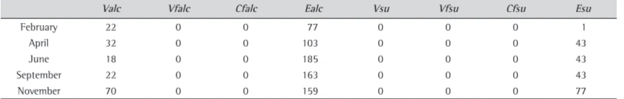
The new model minimizes variance with production constraints; the results obtained are shown in Table 3.
These results are obtained considering the risk minimization at the final period – February 2007. When the risk is minimized at each decision making moment, the results are presented in Table 4.
In this case, the model does not adopt strategies in the futures market and considers an inventory policy to meet a possible future demand, when prices are higher. All sugar production is directed to the warehouses, as it may generate a greater gain in the future, for example, in February of the following year, when higher prices are expected due to seasonality. The sugar demand was not met as the model as it would reduce the wealth in the period.
The significant change in the results, due to the introduction of production constraints, shows the importance of adopting models which consider the productive system. A decision based on traditional hedge ratios models presented in the literature would lead to strategies that could be useless from practical point of view.
After analyzing results from the wealth maximization and variance minimization separately, the model considering both objectives was implemented. The importance of risk and return varies according to the risk aversion parameter η, which reflects the producer’s aversion to risk. This article arbitrarily
considered η = 0.5, and it was possible to study the behavior of the efficient frontier according to this parameter what is out of scope in this study. The constraints of the model are the same used in the previous cases, representing the productive system constraints. The results obtained for the optimization only in the last period are shown in Table 5.
On maturity date the spot and future prices should be equal. However throughout the existence of the futures contract, the spot price is lower than the futures price for most assets. This does not necessarily occur in the case of the agricultural commodities markets. In these markets the spot price is sometimes greater than the future price, falling until the maturity, when both prices coincide. This phenomenon is known as backwardation and it is well-known in literature. The theory regarding backwardation considers that the prices of commodities futures contracts lie below the prices in the spot market as a result of the risk aversion of investors who pay a risk premium for the right to purchase a commodity for a certain price in the future. Geman (2005) presents the level of available inventory as one of the possible causes for the existence of this risk premium.
In the situation analyzed in this article, the model recommends the future purchase, as spot and future prices are in backwardation in the period considered. If the producer realizes this purchase operation of the futures market will lead to profits resulting from daily adjustments he/she will use the futures market with no need of physical delivery. The majority of the production is allocated in alcohol, because the profit obtained with its production is greater than that obtained with sugar. Nevertheless, due to productive constraints, the model is not able to produce only alcohol.
Table 1. Results of wealth maximization in t = H (%).
Valc Vfalc Cfalc Ealc Vsu Vfsu Cfsu Esu
February 0 0 95 0 0 0 57 0
April 0 0 51 0 12 24 50 64
June 30 0 56 70 11 6 50 46
September 31 0 44 39 12 2 50 32
November 39 0 50 0 17 8 50 8
Table 2. Results of wealth maximization in the whole period (%).
Valc Vfalc Cfalc Ealc Vsu Vfsu Cfsu Esu
February 70 0 100 0 30 0 100 0
April 70 0 100 30 0 0 100 0
June 70 0 100 60 0 0 100 0
September 60 0 0 0 0 0 100 0
When optimization is considered for all decision making periods, and not only for the horizon, the obtained results are presented in Table 6.
In this case alcohol spot sales exceed sugar spot sales due to the greater profit margins obtained in the spot market. Alcohol is bought in futures market with no interest in the physical commodity delivery. This results from the relation between spot and future prices what enables the plant owner to profit with daily adjustments. The same does not occur in the case of sugar, what could lead to the operation of futures sales. The optimization model identifies that the profit margins with sugar are not so high and directs the production to alcohol. Once again, the model chooses not to meet demand to favor the wealth obtained along the period.
When the objective was to minimize variance minimization the model has not chosen strategies in the futures market. Sales in the futures market could
be used to reduce risks, but this strategy was not considered as sugar spot prices have been higher than the future ones. It would be advantageous to store the product or sell it in the spot market, considering that this operation in the future could not be used for protection against risks. However, when analyzing wealth maximization the model indicates the future purchase of this commodity because of the daily adjustments to be received. Considering an objective function that integrates risk and wealth, the model suggests the utilization of inventories for protection against risks of price fluctuation and of the futures market for the maximization of gains.
5. Conclusion
The proposed model is useful for decisions regarding hedging in the sugar & alcohol market. Most models in the literature analyze hedging strategies
Table 3. Variance minimization in t = H (%).
Valc Vfalc Cfalc Ealc Vsu Vfsu Cfsu Esu
February 0 0 0 88 0 0 0 12
April 1 0 0 87 1 0 0 111
June 1 0 0 180 43 43 0 30
September 11 0 0 170 14 14 0 2
November 70 0 0 142 0 0 0 59
Table 4. Variance minimization in the whole time period (%).
Valc Vfalc Cfalc Ealc Vsu Vfsu Cfsu Esu
February 22 0 0 77 0 0 0 1
April 32 0 0 103 0 0 0 43
June 18 0 0 185 0 0 0 43
September 22 0 0 163 0 0 0 43
November 70 0 0 159 0 0 0 77
Table 5. Wealth maximization and variance minimization in t = H (%).
Valc Vfalc Cfalc Ealc Vsu Vfsu Cfsu Esu
February 70 0 100 0 30 0 100 0
April 70 0 100 30 0 0 100 0
June 70 0 100 60 0 0 100 0
September 60 0 0 0 0 0 100 0
November 70 0 0 0 30 0 100 0
Table 6. Wealth and variance optimization in the whole period (%).
Valc Vfalc Cfalc Ealc Vsu Vfsu Cfsu Esu
February 70 0 100 10 20 0 0 0
April 70 0 100 40 0 0 0 0
June 70 0 100 70 0 0 0 0
September 70 0 0 0 0 0 0 0
without considering production constraints and hold little practical application. This study verified that the models proposed to build hedging strategies are deficient for not considering the constraints of the productive system.
This model has been developed to deal with the by-products resulting from the production of sugar and alcohol, such as bagasse and energy. However there were no data unavailable and it was not possible to perform computational tests.
Based on the producer’s interests it is possible to build strategies for financial protection. The use of the sugar futures market as an instrument for reduction of the price risk to the plant owner is useful, allowing financial protection and significant gains with purchases in the futures market.
Although scenarios were simulated for alcohol and sugar - aiming to keep the correlation between them through Cholesky factorization - the use of estimation models of bivariate parameters or even conditional models such as ARCH or GARCH could be analyzed. Other future works would be: alternative implementations of scenarios tree generation; analysis of problems with different by-products; the use of swap and options to create strategies and the use of alternative risk measures.
References
CHEN, S. S.; LEE, C. F.; SHRESTHA, K. Futures hedge ratios: a review. The Quarterly Review of Economics and Finance, v. 43, p. 433-465, 2003. http://dx.doi.org/10.1016/ S1062-9769(02)00191-6
COLLINS, R. A. Toward a positive economic theory of hedging. American Journal of Agricultural Economics, v. 79, n. 2, p. 488-499, 1977. http://dx.doi.org/10.2307/1244146
GARCIA, P.; LEUTHOLD, R. M. A selected review of agricultural commodity futures and options markets. European Review of Agricultural Economics, v. 31, p. 235-72, 2004. http://dx.doi.org/10.1093/erae/31.3.235
GEMAN, H. Commodities and commodity derivatives: modeling and pricing for agriculturals, metals and energy. England: Wiley, 2005.
GEMAN, H.; OHANA, S. Time-consistency in managing a commodity portfolio: a dynamic risk measure approach. Journal of Banking & Finance, v. 32, p. 1991-2005, 2008.
http://dx.doi.org/10.1016/j.jbankfin.2007.05.020 GULPINAR, N.; RUSTEM, B.; STTERGREN, R. Simulation and
optimization approaches to scenario tree generation. Journal of Economic Dynamics and Control, v. 28, n. 7, p. 1291-1315, 2004. http://dx.doi.org/10.1016/S0165-1889(03)00113-1
JOHNSON, L. L. The theory of hedging and speculation in commodity futures. Review of Economic Studies, v. 27, p. 139-151, 1960. http://dx.doi.org/10.2307/2296076 LUENBERGER, D. G. Investment science. New York: Oxford
University Press, 1997.
SCHWARTZ, E. S. The stochastic behavior of commodity prices: implications for valuation, and hedging. The Journal of Finance v. 52, n. 3, p. 923-973, 1997. http:// dx.doi.org/10.2307/2329512
SCHWARTZ, E. S.; SMITH, J. E. Short-term variations, and long-term dynamics in commodity prices. Management Science, v. 46, n. 7, p. 893-911, 2000. http://dx.doi. org/10.1287/mnsc.46.7.893.12034
TOMEK, W. G.; PETERSON, H. H. Risk management in agricultural markets: a review. Journal of Futures Markets, v. 21, n. 10, p. 953-985, 2001. http://dx.doi. org/10.1002/fut.2004
TSENG, C.; BARZ, G. Short-term generation asset valuation: a real options approach. Operations Research, v. 50, n. 2, p. 297-310, 2002. http://dx.doi.org/10.1287/ opre.50.2.297.429