doi: 10.1590/0101-7438.2014.034.02.0237
THE LEVERAGE EFFECT AND THE ASYMMETRY OF THE ERROR DISTRIBUTION IN GARCH-BASED MODELS:
THE CASE OF BRAZILIAN MARKET RELATED SERIES
Daniel de Almeida and Luiz K. Hotta*
Received September 22, 2012 / Accepted October 14, 2013
ABSTRACT.Traditional GARCH models fail to explain at least two of the stylized facts found in financial series: the asymmetry of the distribution of errors and the leverage effect. The leverage effect stems from the fact that losses have a greater influence on future volatilities than do gains. Asymmetry means that the distribution of losses has a heavier tail than the distribution of gains. We test whether these features are present in some series related to the Brazilian market. To test for the presence of these features, the series were fitted by GARCH(1,1), TGARCH(1,1), EGARCH(1,1), and GJR-GARCH(1,1) models with standardized Studenttdistribution errors with and without asymmetry. Information criteria and statistical tests of the significance of the symmetry and leverage parameters are used to compare the models. The estimates of the VaR (value-at-risk) are also used in the comparison. The conclusion is that both stylized facts are present in some series, mostly simultaneously.
Keywords: asymmetry in volatility models, asymmetric Garch family models, VaR (Value-at-Risk).
1 INTRODUCTION
Two important features usually found in time series of asset returns are the presence of volatil-ity clustering and the high kurtosis. Here volatilvolatil-ity is considered as the conditional variance, al-though some authors define it as the conditional standard deviation. The most popular model used in the literature to explain these two stylized facts is the generalized autoregressive conditional heteroskedastic (GARCH) model of Bollerslev (1986) [3] with symmetric errors (normal or Stu-dentt distributions). However, these traditional GARCH models cannot explain some stylized facts found in financial time series. Two important unexplained facts are the skewness, or asym-metry, in the distribution of the errors and the leverage effect. The former consists of losses having a distribution with a heavier tail than gains. Simkowitz & Beedles (1980) [18], Kon (1984) [10], among others drew the attention to the skewness in such distribution. French et al. (1987)
*Corresponding author
[8] found that the conditional asymmetry coefficient significantly differs from zero in the stan-dardized residuals when ARCH family models were fitted to the daily returns of the Standard & Poor 500 (S&P) series. The leverage effect, originally introduced by Black (1976) [2], takes into account that losses have a greater influence on future volatility than do the gains. However, no study has tested yet for the simultaneous presence of these two effects, especially for Brazilian related series.
The aim of the present paper is to verify if these stylized facts are present in some market indices related to the Brazilian market and five of the most important stocks traded in the S˜ao Paulo Stock Exchange (BOVESPA). The indices considered are the Ibovespa (IBV, Brazil), MERVAL (Argentina), and S&P (USA), and the five stocks are Ita´u-Unibanco (Ita´u), Vale PNA (Vale), Petrobr´as PN (Petro), Banco do Brasil ON (BB), and Bradesco PN (Brad), in the period from February 1st, 2000 to February 1st, 2011. After filtering the return series with AR(1) models, we fitted the GARCH(1,1), TGARCH(1,1), EGARCH(1,1), and GJR-GARCH(1,1) models with standardized Studentt and standardized asymmetric Studentt innovations, for a total of eight models.
Three methods are used to compare the models. The first one uses the Akaike information crite-rion (AIC) (Akaike, 1974 [1]), the Bayesian information critecrite-rion (BIC) (Schwarz, 1978 [17]), and the Hannan and Quin information criterion (HQ) (Hannan & Quinn, 1979 [11]), to select the best model. The second method tests the significance of the symmetry and leverage parame-ters. The third method compares the value at risk (VaR) estimated by the eight models treated. A model is considered adequate if the VaR estimates have the desired properties. Section 2 presents three GARCH family models which have leverage effect and the asymmetric distribution used to model the error term. Section 3 presents the methods used to compare these models and Section 4 presents some applications. Our concluding remarks are in Section 5.
2 ARMA-GARCH MODELS
Denoting the returns byrt, this series is first filtered by an ARMA model (1), yielding residuals εt, serially uncorrelated, but not necessarily independent. In (2)-(4), the seriesεt is fitted by a conditional volatility model. We can write this class of models as
rt = µt+εt (1)
εt = σtzt (2)
µt = c(µ|t−1) (3)
σt2 = h(µ, η|t−1), (4)
wherec(.|t−1)andh(.|t−1)are functions oft−1 = {rj,j ≤ t −1}, and zt is an inde-pendent and identically distributed (i.i.d.) process, indeinde-pendent of t−1, with E(zt) = 0 and Var(zt) = 1. In the ARMA-GARCH model, the residuals are modeled by the generalized au-toregressive conditional heteroskedasticity (GARCH) model and the shapes of the functions c(.|t−1) and h(.|t−1) are defined by the orders of the ARMA and GARCH models,
For example, in the AR(1)-GARCH(1,1) model, the mean and the volatility given by (3) and (4), respectively, are
µt = µ+φrt−1 (5)
σt2 = ω+αε2t−1+βσt2−1, (6)
with|φ| <1 andω >0. The conditionsα, β ≥ 0,α+β <1, which are sufficient conditions for the process to be stationary and have finite variance, therefore, are usually adopted.
2.1 The leverage effect
The leverage effect is caused by the fact that negative returns have a greater influence on future volatility than do positive returns. For a good comparison among several GARCH models with leverage effect, see Rodr´ıguez & Ruiz (2012) [16]. In this paper, we consider three of the most popular models to represent it: the EGARCH, TGARCH, and GJR models.
In the EGARCH model (Nelson, 1991 [15]), the conditional volatility is given by
ln(σt2)=ω+γEzt−1+α{|zt−1| −E(|zt−1|)} +βln(σt2−1). (7)
Sincezt is an i.i.d. sequence,|εt| − E(|εt|)is also a sequence of i.i.d. random variables with zero mean. γE is a real parameter, such that γE < 0 when negative returns have a greater impact on future volatility than positive returns. Due to the volatility specification in terms of the logarithmic transformation, there are no restrictions on the parameters to ensure positive variance. A sufficient condition for stationarity and finite kurtosis is|β|<1.
The Threshold GARCH (TGARCH)(see Zako¨ıan, 1994 [19]) is a particular case of a nonlin-ear ARCH model and it models the conditional standard deviation instead of the conditional variance. The TGARCH(1,1) is written as
σt =ω+α|εt−1| +βσt−1+γTεt−1. (8)
Ding et al. (1993) [5] proved that, in order to guarantee the positivity ofσt, it is sufficient that ω > 0,α ≥ 0 andγT < α. Furthermore, the model is stationarity ifγT2 < 1−α2−β2−
2αβE(|zt|). For example, ifzt is Gaussian, thenE(|zt|)=
2 π.
The GJR model of Glosten et al. (1993) [9] specifies the conditional variance by
σt2=ω+αεt2−1+βσt2−1+γGI(zt−1<0)ε2t−1, (9)
whereI(.)is equal to 1 when the inequality is satisfied and 0 otherwise. Hentschel (1995) [13] showed thatσt2is positive if
ω >0, α, β, γG≥0. (10)
A sufficient condition for stationarity and finite variance is
2.2 Asymmetry in the errors
In practice, it is generally assumed thatzt ∼N(0,1)orzt ∼tvstandardized, or any distribution
that describes the heavy tails of financial time series. For normal errors and GARCH(1,1), the kurtosis is equal to
K = E(r
4
t) [E(rt2)]2 =
3[1−(α+β)] 1−(α+β)2−2α2
1
>3, (12)
when the fourth moment is defined, i.e., when the denominator is positive. This shows that even when the errorzt has a standard normal distribution andεt follows a GARCH process, the tails ofεtare heavier than normal. However, in empirical series it is often found that the distribution of the error termzt has heavier tails than the normal distribution, and is often replaced by the standardized Studenttdistribution (see, for example, Bollerslev, 1986 [3]).
The standardized Studenttdistribution withν (ν >2)degrees of freedom is given by
g(z)= Ŵ( ν+1
2 )
√
(ν−2)π Ŵ(ν/2)
1+ z
2
(ν−2)
−(ν+21)
, (13)
whereŴis the gamma function.
The distribution given in (13) has skewness coefficient equal to zero and the excess of kurtosis equal to 6/(ν−4),forν >4.
While the high kurtosis of returns is a well established fact, the situation is much more obscure for the symmetry of the distribution ofzt. In this paper, we consider the asymmetric Studentt distribution. There have been several proposals to include asymmetry in the Studentt distribu-tion. Hansen (1994) [12] was the first to use an asymmetric Studentt distribution in modeling financial data. Fern´andez & Steel (1998) [7] proposed a way of introducing asymmetry into any symmetric and unimodal continuous distributiong(.), changing its scale on each side of the mode. Applying this procedure to the Studenttdistribution, one obtains an asymmetric Studentt density. In order to preserve the specifications of the GARCH model, Lambert & Laurent (2001) [14] modified this density to standardize it, that is, to have zero mean and unit variance.
Following Lambert & Laurent (2001) [14], the random variableztis said to follow the standard-ized asymmetric Studentt, denoted by SKST(0,1,ξ, v), with parametersv > 2 (the number of degrees of freedom) andξ >0 (the parameter associated with the skewness), if its density is of the form
f(zt|ξ, v)=
⎧ ⎪ ⎪ ⎪ ⎨ ⎪ ⎪ ⎪ ⎩ 2
ξ+1ξ s g[ξ(szt+m)|v] if zt <−m/s 2
ξ+1ξ s g[(szt+m)/ξ|v] if zt ≥ −m/s,
whereg(.|v)is the density of the standardized symmetric Studenttgiven by (13), and the con-stantsm=m(ξ, v)ands= s2(ξ, v)are, respectively, the mean and standard deviation of the
SKST(m,s2, ξ, v) distribution and can be expressed by
m(ξ, v)= Ŵ( v+1
2 )
√ v−2 √π Ŵ(v
2)
ξ−1 ξ
(15)
and
s2(ξ, v)=
ξ2+ 1 ξ2−1
−m2, (16)
respectively (Fern´andez & Steel, 1998 [7]). The main advantages of this density are its easy implementation and the clear interpretation of its parameters. Ehlers (2012) [6] modeled GARCH model with the error term errors with this distribution and proposed a fully Bayesian approach to estimate the model.
3 CRITERIA FOR COMPARISON OF MODELS
ConsiderT observations of a volatility process and suppose that we want to verify the presence of the leverage effect and of asymmetry in the perturbations. In order to do this, we use the following eight models: GARCH, TGARCH, EGARCH, and GJR-GARCH with standardized symmetric and asymmetric Studenttdistributions. In this section, we present the three criteria used to select the most appropriate model.
Information criteria. There are several information criteria suggested in the literature to se-lect a model. In this paper, we consider the AIC, BIC, and HQ criteria. These criteria are the likelihood penalized by different functions of the number of parameters of the model.
Testing hypotheses. By fitting the GJR-GARCH model with asymmetric Studentt distribu-tion, for example, we have as special cases a model without leverage whenγG =0 and a model with symmetric innovations when the skewness parameter (ξ) is equal to 1. Thus we can use hypothesis testing to verify the presence or absence of these two stylized facts. We can follow the same procedure with GARCH, TGARCH, and EGARCH models.
The third criterion uses the VaR at the 95% and 99% levels to test the accuracy of the models in making predictions. We use the conditional prediction interval evaluation procedure of Christof-fersen (1998) [4]. He proposed a likelihood ratio (LR) test to test the null hypothesis that a statistical method (the model) is good for prediction purpose. This test is defined as follows.
3.1 The likelihood ratio test for the conditional coverage
Let(rt)1≤t≤T be the realization of a series of returns of any financial asset and let[L(p)t|t−1,
U(p))t|t−1] be the corresponding sequence of interval forecast outside the sample, where
L(p)t|t−1andU(p))t|t−1are the lower and upper limits of the forecast intervals at timet, given
the information until timet−1, at the confidence level p. Set the indicator variableItat timet, given information until timet−1, as
It =
1, if rt ∈ [L(p)t|t−1,U(p))t|t−1]
0, if rt ∈ [/ L(p)t|t−1,U(p)t|t−1].
(17)
We say that the sequence of prediction interval,[L(p)t|t−1,U(p))t|t−1], is efficient with respect
to the information set at time t −1 (t−1), if E(It|t−1) = p, ∀t if it passes the LR test.
Christoffersen (1998) [4] showed that testingE(It|t−1)= p, for allt, is equivalent to testing
if the sequence (It)1≤t≤T is i.i.d. with a Bernoulli distribution with parameter p, i.e., It ∼ i.i.d. Ber(p). Therefore, a sequence of prediction intervals,[L(p)t|t−1,U(p))t|t−1], has a correct
conditional coverage ifIt ∼Ber(p) i.i.d.,∀t.
In the conditional coverage test, the null hypothesis is that (It)1≤t≤T is independent and E(It|t−1)= p. The test statistics is
L Rcc = −l(p;I1, . . . ,IT)−l(πˆ1;I1, . . . ,IT)], (18)
wherel(θ; ;I1, . . . ,IT)is the log likelihood function, i.e., l(p;I1, . . . ,IT) = (nT) log(θ )+ (T −nT) log(1 −θ ) withnT = Ti=1Ii, andπˆ1 = nT/T. The statistics L Rcc has a χ22 distribution under the null hypothesis.
Equation (18) can be written as the sum of the LR test statistics for the correct unconditional coverage and the LR test statistics for independence (Christoffersen, 1998 [4]). Rejecting the null hypothesis implies that the model is not good for prediction purpose.
4 APPLICATIONS
In this section, we analyze the series of returns of IBV, Merval, S&P, Ita´u, Vale, Petro, BB, and Brad, from February 1st, 2000 to February 1st, 2011, with a total of 12 years. Each series was previously filtered by an ARMA(p,q)model with appropriate orders.
For each dataset we adopted the following procedure.
1. Consider the observations of the returns of the first eight years.
2. Fit all eight models.
3. Verify which model is selected by the AIC, BIC and HQ criteria.
5. Include five more observations and exclude the first five observations.
6. Repeat steps (2) to (5) until the end of the period.
For each series and each model, we fitted around 200 models and estimated around 1,000 VaR values. The number of models and VaR estimates depend upon each series, because we ignored non-trading days.
Tables 1 and 2 indicate how many times each of the eight models were selected by the AIC, BIC, and HQ criteria. The main conclusions are:
• The GARCH model was never selected by any criterion for the IBV, S&P, Ita´u, Petro, or Brad series. For the Merval and Vale series, the GARCH model was only selected by the BIC (60% of the time for the Merval series and 21% for the Vale series); for the BB series the GARCH model was only selected 31% of the time. This means that there is a clear preference of the information criteria for models with the leverage effect.
• For all of the stocks, the GJR was the most selected model by all the criteria. For the Petro and Brad series, it was always the model selected. For the Merval series, the GJR model was always selected by the AIC, in 91% of the cases by the HQ criterion, and 40% by the BIC. The TGARCH was selected most of the time for the IBV series by all criteria, and the EGARCH model was selected most of the time for the S&P series by all criteria.
• For the IBV and S&P series, the criteria selected models with leverage and asymmetric distributions almost all the time. For the Merval, Ita´u, and Brad series, the criteria selected models with leverage and asymmetric distributions most of the time. For the Vale, Petro, and BB series, the criteria selected models with leverage and symmetric distributions most of the time.
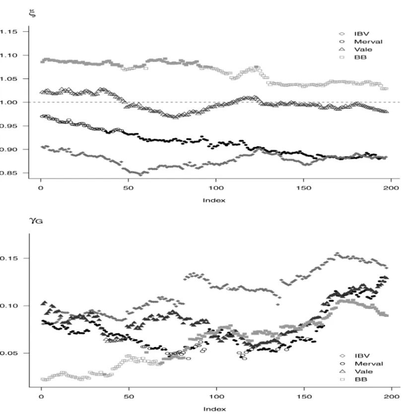
Tables 3 and 4 present, respectively, the percentage of cases where the asymmetry and leverage parameters were significant at the 5% level. Figure 1 presents the estimated asymmetry and leverage parameters in the GJR-GARCH asymmetric model for the IBV, Merval, Vale, and BB series, while Figure 2 presents the results for the Ita´u, S&P, Petro, and Brad series. We do not present the equivalent graphs for the other models, since their behavior is very similar to that of the GJR model. Under the null hypothesis of no asymmetry, one hasξ =1; and under the null hypothesis of no leverage effect,γG =0. We use full symbols to indicate rejection of the null hypotheses at the 5% level. The main conclusions are:
Table 1– Number of times the model was selected by the AIC, BIC, and HQ criteria. Panels 1–8 correspond to the IBV, Merval, S&P, Ita ´u, Vale, Petro, BB, and Brad series, respectively. sym., asym. = standardized symmetric and asymmetric Studenttinnovations, respectively.
Criterion GARCH GJR EGARCH TGARCH
sym. asym. sym. asym. sym. asym. sym. asym.
AIC 0 0 0 30 0 26 0 141
BIC 0 0 0 30 8 18 3 138
HQ 0 0 0 30 0 26 0 141
AIC 0 0 20 176 0 0 0 0
BIC 66 52 37 41 0 0 0 0
HQ 0 17 46 133 0 0 0 0
AIC 0 0 0 13 0 142 0 46
BIC 0 0 0 13 22 120 0 46
HQ 0 0 0 13 6 136 0 46
AIC 0 0 0 92 0 40 0 65
BIC 0 0 25 53 49 0 38 32
HQ 0 0 9 81 10 30 6 61
AIC 0 0 183 0 0 0 14 0
BIC 42 0 141 0 0 0 14 0
HQ 0 0 183 0 0 0 14 0
AIC 0 0 38 159 0 0 0 0
BIC 0 0 197 0 0 0 0 0
HQ 0 0 152 45 0 0 0 0
AIC 0 42 69 86 0 0 0 0
BIC 81 0 116 0 0 0 0 0
HQ 1 58 102 36 0 0 0 0
AIC 0 0 12 185 0 0 0 0
BIC 0 0 111 86 0 0 0 0
HQ 0 0 62 135 0 0 0 0
• The asymmetry in the errors was detected in all the cases for all models for the IBV and S&P series, and in approximately 75%, 70%, and 50% of the cases for the Merval, Brad, and BB series, respectively. For the Vale series, the null hypothesis was never rejected. For the Ita´u and Petro series, the percentage depended on the model. For the Ita´u series, the detection of asymmetry varied from 99.5% for the GARCH model to 74.6% for the TGARCH model, while for the Petro series the percentages varied from 34.5% for the GJR model to 9.1% for the EGARCH model.
Table 2– Percentage of selection of a model with leverage (GJR, EGARCH, TGARCH) and without leverage (GARCH), and with and without asymmetric innovations. The left side panels 1–4 correspond to the IBV, S&P, Vale, and BB series, respectively. The right side panels 1–4 correspond to the Merval, Ita ´u, Petro, and Brad series, respectively. sym., asym. = standardized symmetric and asymmetric Studenttinnovations, respectively.
Left panel Right panel
Criterion Leverage Innovation Leverage Innovation
without with sym. asym. without with sym. asym.
AIC 0.00 100.0 0.00 100.0 0.00 100.0 10.20 89.80
BIC 0.00 100.0 5.58 94.42 59.90 40.10 52.55 47.45
HQ 0.00 100.0 0.00 100.0 23.35 76.65 23.47 76.53
AIC 0.00 100.0 0.00 100.0 0.00 100.0 0.00 100.0
BIC 0.00 100.0 10.95 89.05 0.00 100.0 56.85 43.15
HQ 0.00 100.0 2.99 97.01 0.00 100.0 12.69 87.31
AIC 0.00 100.0 100.0 0.00 0.00 100.0 19.29 80.71
BIC 21.32 78.68 100.0 0.00 0.00 100.0 100.0 0.00
HQ 0.00 100.0 100.0 0.00 0.00 100.0 77.16 22.84
AIC 21.32 78.68 35.03 64.97 0.00 100.0 6.09 93.91
BIC 41.12 58.88 100.0 0.00 0.00 100.0 56.35 43.65
HQ 29.95 70.05 52.28 47.72 0.00 100.0 31.47 68.53
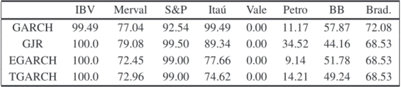
Table 3– Percentage of times the skewness parameter of the asymmetric Studentt distribution were significant at the 5% level.
IBV Merval S&P Ita ´u Vale Petro BB Brad. GARCH 99.49 77.04 92.54 99.49 0.00 11.17 57.87 72.08 GJR 100.0 79.08 99.50 89.34 0.00 34.52 44.16 68.53 EGARCH 100.0 72.45 99.00 77.66 0.00 9.14 51.78 68.53 TGARCH 100.0 72.96 99.00 74.62 0.00 14.21 49.24 68.53
Table 4– Percentage of times the leverage parameter of the GJR model was sig-nificant at the 5% level.
Distr. IBV Merval S&P Ita ´u Vale Petro BB Brad.
sym. 100.0 79.70 100.0 100.0 98.98 100.0 68.02 100.0 asym. 100.0 82.74 100.0 100.0 95.94 100.0 66.50 100.0
Figure 1–Estimates of the asymmetry parameter of the error distributions(ξ )and of the leverage parameter
(γG)of the GJR-GARCH model for the IBV, Merval, Vale, and BB series. Full symbols mean rejection of
the null hypothesis at 5%. Under the null hypothesis of no asymmetry, one has(ξ=1); and under the null
hypothesis of no leverage effect,(γG=0).
• There is no meaningful difference in terms of percentage, although the models with asym-metric distributions are generally slightly better.
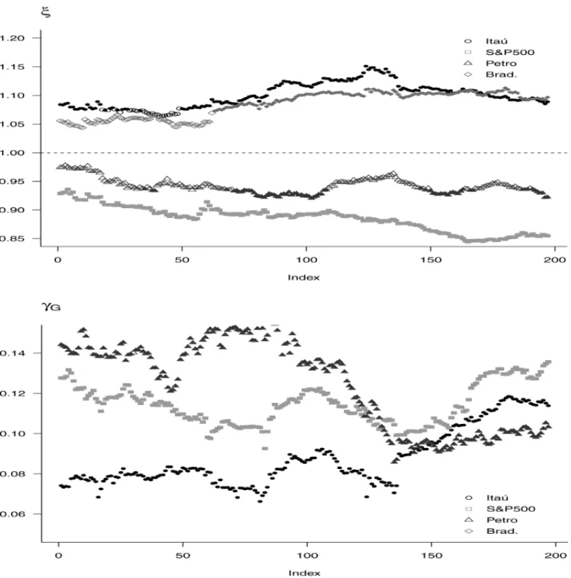
Figure 2–Estimates of the asymmetry parameter of the error distributions(ξ )and of the leverage parameter
(γG)of the GJR-GARCH model for the Ita ´u, S&P, Petro and Brad series. Full symbols mean rejection of
the null hypothesis at 5%. Under the null hypothesis of no asymmetry, one has(ξ=1); and under the null
hypothesis of no leverage effect,(γG=0).
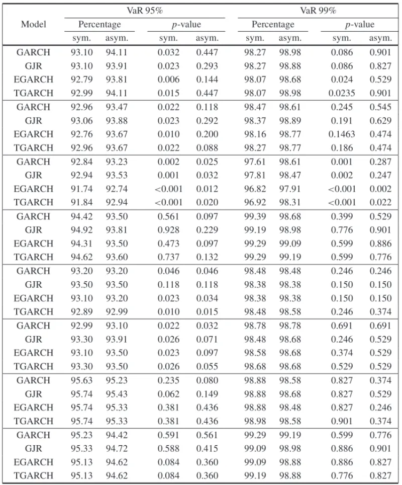
• For the 95%-VaR, the models with asymmetric error distribution, except for the Vale, Petro (for GARCH model), and S&P series, pass the LR test at the 5% level. When we consider the symmetric error distribution, all the models fail for the IBV, Merval, S&P, Vale (except for GJR), and Petro series.
Table 5– Percentage of cases with loss larger than the VaR and thep-value of the LR test for the conditional 95%-VaR and 99%-VaR. Panels 1–8 correspond to the IBV, Merval, S&P, Ita ´u, Vale, Petro, BB, and Brad series, respectively.
VaR 95% VaR 99%
Model Percentage p-value Percentage p-value
sym. asym. sym. asym. sym. asym. sym. asym.
GARCH 93.10 94.11 0.032 0.447 98.27 98.98 0.086 0.901
GJR 93.10 93.91 0.023 0.293 98.27 98.88 0.086 0.827
EGARCH 92.79 93.81 0.006 0.144 98.07 98.68 0.024 0.529
TGARCH 92.99 94.11 0.015 0.447 98.07 98.98 0.0235 0.901
GARCH 92.96 93.47 0.022 0.118 98.47 98.61 0.245 0.545
GJR 93.06 93.88 0.023 0.292 98.37 98.89 0.191 0.629
EGARCH 92.76 93.67 0.010 0.200 98.16 98.77 0.1463 0.474
TGARCH 92.96 93.67 0.022 0.088 98.27 98.77 0.186 0.474
GARCH 92.84 93.23 0.002 0.025 97.61 98.61 0.001 0.287
GJR 92.94 93.53 0.001 0.032 97.81 98.47 0.002 0.247
EGARCH 91.74 92.74 <0.001 0.012 96.82 97.91 <0.001 0.002 TGARCH 91.84 92.94 <0.001 0.020 96.92 98.31 <0.001 0.022
GARCH 94.42 93.50 0.561 0.097 99.39 98.68 0.399 0.529
GJR 94.92 93.81 0.928 0.229 99.19 98.98 0.776 0.901
EGARCH 94.31 93.50 0.473 0.097 99.29 99.09 0.599 0.886
TGARCH 94.62 93.60 0.737 0.132 99.29 99.19 0.599 0.776
GARCH 93.20 93.20 0.046 0.046 98.48 98.48 0.246 0.246
GJR 93.50 93.50 0.118 0.118 98.38 98.38 0.150 0.150
EGARCH 93.10 93.20 0.023 0.034 98.38 98.38 0.150 0.150
TGARCH 92.89 92.99 0.010 0.015 98.48 98.58 0.246 0.374
GARCH 92.99 93.10 0.022 0.032 98.78 98.78 0.691 0.691
GJR 93.30 93.91 0.026 0.071 98.48 98.68 0.246 0.529
EGARCH 93.10 93.50 0.023 0.097 98.58 98.68 0.374 0.529
TGARCH 93.30 93.50 0.026 0.055 98.68 98.68 0.529 0.529
GARCH 95.63 95.23 0.235 0.080 98.88 98.58 0.827 0.374
GJR 95.74 95.43 0.062 0.149 98.88 98.68 0.827 0.529
EGARCH 95.74 95.33 0.381 0.436 98.88 98.48 0.827 0.246
TGARCH 95.74 95.33 0.381 0.436 98.98 98.58 0.901 0.374
GARCH 95.23 94.42 0.591 0.561 99.29 99.19 0.599 0.776
GJR 95.33 94.72 0.588 0.415 99.09 98.98 0.886 0.901
EGARCH 95.13 94.62 0.084 0.360 99.09 98.88 0.886 0.827
TGARCH 95.13 94.62 0.084 0.360 99.19 98.88 0.776 0.827
5 CONCLUDING REMARKS
the AIC, BIC, and HQ information criteria, and by using hypothesis testing. In both methods, we found evidence that the two stylized facts are present in most of the series analyzed. In the third method, we compared the VaR estimates and found that in VaR estimation, the models with asymmetric errors performed much better than those with symmetric distributions, in terms of the LR test.
ACKNOWLEDGMENTS
This work was partially supported through grants 2008/51097-6 and 2011/02881-9, S˜ao Paulo Research Foundation (FAPESP), and grants from CAPES and CNPq.
REFERENCES
[1] AKAIKEH. 1974. A new look at the statistical model identification.IEEE Transactions on Automatic Control,19: 716–722.
[2] BLACKR. 1976. Studies in stock price volatility changes. Proceedings of the 1976 Meeting of the American Statistical Association, Business and Economics Statistics Section, 177–181.
[3] BOLLERSLEVT. 1986. Generalized autoregressive conditional heteroskedasticity.Journal of Econo-metrics,31: 307–327.
[4] CHRISTOFFERSENP. 1998. Evaluating interval forecasts.International Economic Review,39: 841– 862.
[5] DINGZ, ENGLERF & GRANGERCWJ. 1993. A long memory property of stock market return and a new model.Journal of Empirical Finance,1: 83–106.
[6] EHLERSRS. 2012. Computational tools for comparing asymmetric GARCH models via Bayes fac-tors.Mathematics and Computers in Simulation,82: 858–867.
[7] FERNANDEZ´ C & STEELM. 1998. On Bayesian modelling of fat tails and skewness.Journal of the American Statistical Association,93: 359–371.
[8] FRENCH KG, SCHWERT W & STAMBAUGH RF. 1987. Expected stock returns and volatility. Journal of Financial Economics,19: 3–29.
[9] GLOSTENLR, JAGANNATHANR & RUNKLEDE. 1993. On the relation between the expected value and the volatility of the nominal excess return on stocks.Journal of Finance,48: 1779–1801.
[10] KONS. 1982. Models of stock returns, a comparison.Journal of Finance,39: 147–165.
[11] HANNANEJ & QUINNBG. 1979. The determination of the order of an autoregression.Journal of the Royal Statistical Society B,41: 190–195.
[12] HANSENB. 1994. Autoregressive conditional density estimation.International Economic Review,
35: 705–730.
[13] HENTSCHELL. 1995. All in the family nesting symmetric and asymmetric GARCH models.Journal of Financial Economics,39: 71–104.
[15] NELSONDB. 1991. Conditional heteroskedasticity in asset returns: A new approach.Econometrica,
59: 347–370.
[16] RODR´IGUEZMJ & RUIZE. 2012. Revisiting several popular GARCH models with leverage effect: Differences and similarities.Journal of Financial Econometrics,10: 637–668.
[17] SCHWARZGE. 1978. Estimating the dimension of a model.Annals of Statistics,6: 461–464.
[18] SIMKOWITZM & BEEDLESW. 1980. Asymmetric stable distributed security returns.Journal of the American Statistical Association,75: 306–312.
[19] ZAKO¨IANJM. 1994. Threshold heteroskedastic models.Journal of Economic Dynamics and Control,