BLACK SWANS IN THE BRAZILIAN STOCK MARKET
Hugo Jacob Lovisolo
1and Ricardo Pereira Cˆamara Leal
2* Received December 15, 2011 / Accepted January 23, 2013ABSTRACT.This study analyzes extreme values in the daily returns of 45 Brazilian stocks between 2 Jan-uary 1995 and 18 March 2009. The incidence of observations outside the range of three standard deviations from the mean is at least five times greater than under the normal distribution. The occurrence of extreme values in the upper tail is 1.13 times higher than in the lower. The average of the extreme positive returns is higher than that of extreme negative returns. Half percent of the days determined the outcome of the in-vestment. Extreme values are at least±7%. Investors should assess whether they will keep their holdings when returns of such magnitude occur. The characteristics of empirical distributions of stock returns favor the passive investor and the use of weight constraints in portfolio allocation models.
Keywords: extreme values, normal distribution, stock risk and return.
1 INTRODUCTION
It is a well-known fact that the returns of financial assets are not normally distributed. Mandelbrot (1963) showed that financial returns have a stable Pareto distribution withαless than 2, which implies an unknown variance and makes the assumption of normality difficult. It is not valid to assume that 68.26% of observations are found between ±1σ (standard deviation), 95.44% between±2σ, and 99.73% between±3σ. Investors may underestimate their risk exposure if they assume that returns follow a normal distribution. This creates considerable problems for the classic mean-variance optimization proposed by Markowitz (1952) because it presumes that returns follow a normal distribution.
The consequences of the normality assumption may also vary according to the time horizon of an investment. Values are concentrated in the tails of the distribution and clustered around the mean when the distribution of returns is leptokurtic. As a consequence, Estrada (2008, 2009) af-firms that returns from a few days are decisive determinants of the value accumulated in a stock
*Corresponding author
1Chief Executive Officer at Notoria HB – Soluc¸˜oes Inteligentes, R. Alexandre Ferreira, 291, 22470-220 Rio de Janeiro, RJ, Brazil. Phone: +55 (21) 2113-0456. E-mail: [email protected]
2Full Professor of Finance at the Coppead Graduate School of Business, Federal University of Rio de Janeiro – UFRJ, R. Pascoal Lemme, 355, 21941-918 Rio de Janeiro, RJ, Brazil. Phone: +55 (21) 2598-9800.
portfolio. The impact of these extreme values may possibly be reduced if the investment hori-zon is longer. Perhaps a long-term investor is not very concerned about short-term fluctuations if changes in asset prices tend to balance out after long periods. Long-term investors thus consider that the distribution of returns is Gaussian, in which only the mean and variance of the distri-bution matter. Short-term investors, however, believe that their gains are obtained during large market fluctuations.
The leptokurtosis of returns produces what Taleb (2007) called “black swans”: rare events with a great impact. According to the author, understanding the reasons behind extreme variations in asset values and their effects on investment returns enables investors to protect themselves against catastrophic losses and achieve higher returns than those obtained by investors who ex-pose themselves to high volatility. Haugen & Baker (1996) affirm that high volatility assets do not provide the highest historical returns. Tversky & Kahneman (1991) conclude that the probability of loss has a greater influence on the preferences of investors than potential gains. DeMiguel
et al. (2009) present evidence that has devastating implications for mean-variance optimization and many of the subsequent refinements designed to deal with the problem of optimization input parameters error. They compared 14 methods for obtaining the weights of efficient portfolios – those with greater expected returns for each level of risk – and concluded that none of them is superior to the na¨ıve strategy of investing an equal amount in each asset.
This study takes these findings as its starting point to describe the behavior and financial impact of extreme stock returns in the Brazilian market. Estrada (2008) affirms that being out of the market in the few days of the best performance of emerging market stocks bring serious financial consequences to investors. This article draws from the recent portfolio allocation literature and its descriptive findings to suggest how investors may acquire a better understanding of the risks to which they are exposed and which usable and practical portfolio models better fit the charac-teristics of the data, thus increasing their probability of gains, and also points out the limitations of the traditional mean-variance optimization.
The characteristics of the distribution of returns, as inputs for portfolio decision making, are important for the design of the most adequate methods to handle the data as well as for the interpretation of the outcomes. We hope that this paper contributes to this literature by exposing important distributional characteristics of the Brazilian data and their implications for portfolio selection methods that investors in Brazil and wherever data show similar patterns can use.
This article proceeds with an exam of the previous literature in Section 2, the description of the sample and method in Section 3, and the discussion of the results in the following section. Section 5 concludes.
2 BACKGROUND
assump-tion presume a distribuassump-tion of informaassump-tion that may not be consistent with what is observed. In an article about the implications of the 2008 financial crisis for the theory of finance, The Economist(2009) quoted Myron Scholes as saying that many of the models used in financial markets were good but their input parameters were faulty because they reflected a view of the world that underplayed risk. Scholes affirmed that systemic risk was not duly taken into account and that decisions regarding exposure to risk made individually in each institution did not ad-equately consider the relations between different types of assets and the similar steps taken by these same institutions to cut their losses. Perhaps the magnitude of systemic risk was one of the “black swans” of the 2008 crisis. However, its lessons are being learnt. The all-embracing and severe Dodd-Frank Law, approved by the US Congress at the end of 2009, introduced a “regulator” of systemic risk, the Financial Stability Oversight Council, which, according theThe Economist, was also being considered by various other countries.
The use of mathematical models in portfolio selection decisions has been the object of semi-nal articles published in management science/operations research periodicals, as illustrated by Osborne (1959), Sharpe (1963), Fama (1965), Brada et al.(1966), and Ziembaet al. (1974). More recent articles by Huddartet al. (2009), Yanget al. (2010), and Turner & Weigel (1992), among others, and several chapters of the series titled “Handbooks in Operations Research and Management Science” published by Elsevier, of which the portfolio theory survey by Constan-tinides & Malliaris (1995) is good example, indicate that the topic is current in the field. The Brazilian operations research literature also includes articles concerned with the distribution of financial assets returns, their extreme values, and portfolio selection, as exemplified by Costa & Baidya (2001), Moretti & Mendes (2003), and Ferreiraet al.(2009).
Emerging markets and Brazilian return data analysis have been performed in the literature, with a particular interest in non-normality and extreme values. Ribeiro & Leal (2002) analyzed the fractal structure of emerging markets and, as would be expected, discarded the normality hypoth-esis in favor of more general cases of stable Pareto distributions. Torreset al.(2002) performed a careful investigation into the informational efficiency of the Brazilian stock market and rejected both the linearity and the normality of observed returns. Costa & Baidya (2001) arrived at sim-ilar conclusions in their study of the behavior of six of the more liquid shares in the Brazilian stock market and posit that returns are linearly and non-linearly dependent, but do not succeed in fitting models to their autocorrelated sample. Moretti & Mendes (2003) analyzed the problems of fitting bivariate extreme value models to financial data, Brazilian and foreign, to account for simultaneous extreme values.
The non-normality and high incidence of extreme values in stock market return series also has consequences for portfolio allocation and its models. DeMiguelet al. (2009) present evidence that a simple equally weighed portfolio, in which each asset corresponds to a proportion of 1/n
of the initial investment, forn assets, beats all of the 14 more sophisticated portfolio allocation models using US and other developed countries data that they employed. The naive 1/n port-folios outperformed even some robust portfolio allocation models included in their tests. The authors concluded that a window of 3,000 months would be necessary for a mean-variance opti-mization method to beat the naive portfolio.
DeMiguelet al. (2009) also considered the global minimum variance portfolio (GMVP), that does not demand expected return inputs. Thom´e Netoet al.(2011) analyzed the performance of the GMVP and 1/n portfolios according to several constraints on the maximum weights an asset could attain. They concluded that the GMVP with no short selling and weights limited to no more than 10 percent and the 1/noffered better risk adjusted performance than other GMVP allocations with larger weight constraints or unconstrained, the Ibovespa index, and several actively managed stock funds. They found no statistical difference between the performance of 1/nportfolios and the GMVP portfolios with weights constrained to 10 percent. The authors studied the returns of the most liquid Brazilian stocks between January 1998 and December 2008, with rebalancing every four months, in synchrony with the Ibovespa index rebalancing. Behret al. (2013) considered the role of constraints in a comparative analysis of optimized portfolios relative to naive 1/nportfolios. Their constraints were based on shrinkage theory. They find that their approach was the only one to outperform the Sharpe ratio of naive allocations.
Extreme values may bring about very serious financial consequences for investors. Stock return data contains many more extreme values than the predicted under a normal distribution. Being absent from the market in the best return days yields a mediocre financial performance. Ex-treme returns also affect the weights of optimized portfolios while weight constraints, ad hoc or not, alleviate these problems. Equally weighed portfolios are a competitive solution for practical portfolio allocation problems.
3 SAMPLE AND METHOD
Closing stock prices, adjusted for dividends and other payments, were taken from the Bloom-bergrsystem. The stocks of some companies have a smaller number of daily observations be-cause they were not traded on all days of the period studied. Five companies were excluded from the sample because their stock prices were not quoted for long periods (Light ON) or be-cause their price series had consistency problems that could not be resolved by the data provider (Celesc PNA, M.G. Poliest ON, Varig PN, and Forjas Taurus PN). The final sample included 45 companies from 13 industries. The industry with the largest number of companies was the electricity energy, with seven companies, followed by steel and metallurgy with six, the financial and insurance and chemical industries with five, pulp and paper with four and the other nine sectors with no more than two stocks each. The appendix contains a list of companies with their ticker symbols, industry, the number and percentage of days with returns during the period and the means, standard deviations and sum of logarithmic returns for each stock in the sample.
The return of a stockion dayt(ri,t)was calculated as the difference between the price logarithms
on this day and the previous one(ln Pi,t −ln Pi,t−1). The logarithmic returns can be summed to obtain the accumulated return during a period. Logarithmic returns attenuate the effects of extreme values on the form of their empirical distribution, making it more similar to a normal distribution.
The frequency of observed returns was compared with those expected under normality for various areas around and more distant from the mean. The result of the investment undertaken when an investor was not long on the stock on its worst and best days was compared with that of a passive investor who followed a buy and hold strategy. The study examined the 1, 5, 10, 20 and 50 worst or best days. The aim was to investigate whether a few daily returns determined the final result of the investment even when its time horizon was long.
Let T be the number of trading days during a certain period, TG the set of N days with the
largest gains duringT, TP the set of N days with the largest losses duringT, with N equal
to 1, 5, 10, 20 and 50 days. The percentage gain of stocki during periodT(Gi,T)due to not
being invested during theNworst days of the period is given by equation 1. The percentage loss recorded by stockiduring periodT(Pi,T)due to not being invested during theNbest days of the
period is given by equation 2. The denominator of the two equations is the return achieved by a passive investor who remained invested in the stock throughout the whole period. The numerator of equation 1 represents the return of an investor who was not long on the stock precisely on the days when it had its lowest returns. The numerator of equation 2 represents the return achieved by an unlucky investor who was not long on the stock exactly on the days when it had its best returns.
Gi,T =100×
e
PT t=1,t∈/TPri,t
ePTt=1ri,t −1
(1)
Pi,T =100×
e
PT t=1,t∈/TGri,t
ePTt=1ri,t −1
The distance(Di)of the mean return of the set of extreme observations(R¯e,i)in relation to
the mean return of a stock (R¯i)during the period, in units of its standard deviation (σi), was
calculated according to equation 3. The set of extreme observations considered are represented byTG, the set ofN days with the largest gains, andTP, the set ofN days with the largest losses,
withNequal to 1, 5, 10, 20 and 50 days.
Di = ¯
Re,i− ¯Ri
σi (3)
4 RESULTS
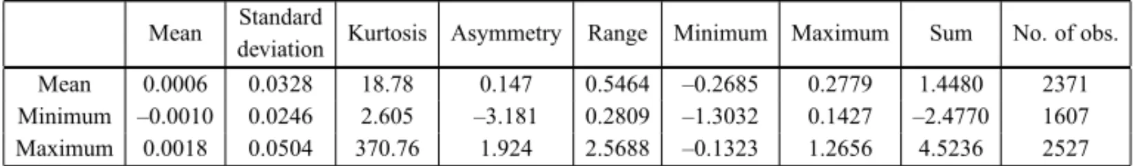
Table 1 presents a summary of the descriptive statistics of the logarithmic returns of each stock. The detailed results for each stock can be obtained from the authors. The appendix contains a list of companies with some of their statistics. There were large differences between the companies in nearly all cases of the descriptive statistics shown. The average of the sum of logarithmic returns during the period was 1.448, or 325.5%, representing the result achieved by a passive investor who invested in an equally weighted portfolio containing the shares in the sample. Seven shares had negative mean daily returns. The mean of daily logarithmic returns of the best performing stock was nearly 19 times greater than that of the stock with the lowest mean positive return. The mean of the five best performing stocks was 677% greater than the mean of the five stocks with the lowest positive appreciation.
Table 1– Summary of the descriptive statistics of the logarithmic returns of each stock.
Mean Standard Kurtosis Asymmetry Range Minimum Maximum Sum No. of obs. deviation
Mean 0.0006 0.0328 18.78 0.147 0.5464 –0.2685 0.2779 1.4480 2371
Minimum –0.0010 0.0246 2.605 –3.181 0.2809 –1.3032 0.1427 –2.4770 1607
Maximum 0.0018 0.0504 370.76 1.924 2.5688 –0.1323 1.2656 4.5236 2527
The largest standard deviation in the sample was almost twice as high as the lowest. The corre-lation between the standard deviations and the mean of the logarithmic returns was−0.39 and suggested an inverse relation between the returns achieved and historical volatility, as indeed found by other authors. As a matter of fact, if the relationship between the returns achieved and historical volatility were monotonic and positive, investors would only choose riskier assets. The coefficient of correlation between these two metrics was negative but not very low and suggested that cases of high risk accompanied by large returns also existed among the companies in the sample. A careful examination of the appendix confirms this. It may be the case that investors who are willing to engage in frequent short-term buying and selling of shares should seek shares with the highest standard deviations, whereas long-term investors should perhaps choose shares with lower standard deviations.
asymmetry are three and zero respectively. Average kurtosis was six times greater than three and minimum and maximum values were 2.605 and 370.75 respectively. Kolmogorov-Smirnov and Jarque-Bera normality tests, whose results are reported in the appendix, also rejected the nor-mality hypothesis for all companies in the sample. Sixteen companies had negative asymmetry coefficients and twenty-nine had positive ones. The average was close to zero, but few stocks had coefficients close to zero. Positive asymmetry is obviously desirable.
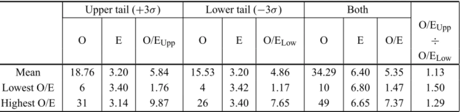
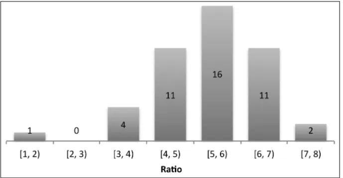
Table 2 presents the number of extreme observations of logarithmic returns compared to the number of extreme values expected if the distribution was normal. Extreme values are those that fall outside three standard deviations above or below the mean, where no more than 0.27% of observations should be under normality. The number of extreme values expected for each stock is the result of the sum of the number of daily observations for the stock in the sample multiplied by 0.00135, which is the proportion of the unit area under the curve in each area above or below three standard deviations from the mean. The average frequency of extreme values was at least five times greater than would be expected under normality. The incidence of extreme values in the upper tail was 1.13 times greater than in the lower one, which had already been indicated by the greater occurrence of positive asymmetry coefficients. The stock with the lowest number of extreme values had 1.47 more than would be expected if the distribution of daily returns were normal. Figure 1 presents the frequency histogram for the ratio of observed to expected returns above or below three standard deviations from the mean for the 45 stocks in the sample. For most of them, the frequency of extreme values was between four and seven times greater than what would be expected under normality.
Table 2– Number of extreme values of observed (O) and expected (E) returns for a normal distribution in the tails(±3σ )between 2 January 1995 and 18 March 2009.
Upper tail (+3σ) Lower tail (−3σ) Both
O/EUpp
O E O/EUpp O E O/ELow O E O/E ÷
O/ELow
Mean 18.76 3.20 5.84 15.53 3.20 4.86 34.29 6.40 5.35 1.13
Lowest O/E 6 3.40 1.76 4 3.42 1.17 10 6.80 1.47 1.50
Highest O/E 31 3.14 9.87 26 3.40 7.65 49 6.65 7.37 1.29
Note: the number of extreme values expected for each stock is the result of the sum of daily observations for the stock in the sample multiplied by 0.00135, which is the proportion of the unit area under the curve in each area above or below three standard deviations from the mean.
Figure 1– Frequency histogram of the ratio between the count of observed and expected returns under normality in the tail region of the distribution, located three standard devi-ations above and below the mean return for 45 Brazilian stocks.
earned five times more than a passive investor. Naturally, very few investors are so lucky or unfortunate in the real world.
What this all shows is that the result of an investment in stocks is determined by a handful of devastating or dazzling days. Mean absolute returns of the ten most devastating days were nearly 230 times greater than the mean returns of all days and were around−14% per day. The mean
accumulated logarithmic return on all days in Table 1 was 1.448. The sum of the mean returns of the ten worst days was approximately−1.5. The difference between these two values was slightly negative and represented the sum of the mean returns in all other days. The sum of the ten best daily returns was approximately 1.6. By subtracting this value from the sum of the mean returns of all other days, one obtains the sum of mean returns of the other days, which was also negative. The mean daily returns of the 50 most devastating days was−9.5%. The mean extreme minimum logarithmic return was around−7%, in the case of losses, and 8% in the case of gains. Daily variations of this size should put an investor on alert. The distance of
±3σ is easily surpassed on days when the market experiences movements of great magnitude. The average distance of the extreme values of each stock from the mean is nearly always greater than 3σ.
Table 3– Mean returns, distance in standard deviations and the effect on the final wealth of the investor of logarithmic returns on the best and worst days of each stock between 2 January 1995 and 18 March 2009.
Best days
1 5 10 20 50
Mean 0.28 0.19 0.16 0.13 0.10
Mean returns Minimum 0.14 0.13 0.11 0.09 0.08
Maximum 1.27 0.44 0.28 0.23 0.17
Distance from Mean 8.2 5.8 4.8 4.0 3.1
the mean in Minimum 4.5 4.1 3.8 3.2 2.4
standard deviations Maximum 25.8 8.9 7.0 5.4 3.9
Percentage Mean 23.16 60.10 78.28 91.86 99.13
reduction in Minimum 13.30 46.71 66.53 84.61 97.77
final wealth Maximum 71.79 88.89 94.92 94.92 99.98
Worst days
1 5 10 20 50
Mean –0.27 –0.18 –0.15 –0.13 –0.10
Mean returns Minimum –1.30 –0.41 –0.26 –0.21 –0.16
Maximum –0.13 –0.12 –0.11 –0.09 –0.07
Distance from Mean –7.9 –5.6 –4.7 –3.9 –2.9
the mean in Minimum –4.5 –4.1 –3.3 –3.3 –2.4
standard deviations Maximum –26.5 –8.4 –6.4 –4.9 –3.4
Percentage Mean 34.07 166.03 409.62 1415.68 21414.62
increase in Minimum 14.15 77.92 188.77 516.22 3020.31
final wealth Maximum 268.09 659.90 1299.10 6645.20 261232.09
1 5 10 20 50
Proportion of Mean 0.04 0.21 0.42 0.85 2.14
total trading Minimum 0.04 0.20 0.40 0.79 1.98
days (%) Maximum 0.06 0.31 0.62 1.24 3.11
Notes: (1) The percentage increase in accumulated wealth in relation to the result obtained by a passive investor at the end of the period was calculated using equation 1; (2) The percentage reduction in accumulated wealth in relation to the result obtained by a passive investor at the end of the period was calculated using equation 2; (3) The distance form the mean in standard deviation units was calculated using equation 3.
with losses of 7% or more on each one, may also decide to sell because they have come to the conclusion that the chances of recovery are small.
losses incurred on disastrous days will be offset by the gains obtained on dazzling ones. The best of worlds, however, would be a situation in which disastrous days were not lumped together with the dazzling days, and have not yet occurred, and investors decide to sell after realizing that they were invested on the best days. It is important that investors observe highly volatile days carefully in order to draw their conclusions and take their decisions accordingly. They should take note of daily returns of±7% because they are the black swans.
Table 4 presents a summary of the comparisons made between the number of occurrences of observations in selected areas of the empirical distribution and the number expected under nor-mality. An examination of Table 4 confirms the leptokurtic characteristics of the empirical dis-tributions, given that both the percentage of values observed in the area close to the mean and the percentage of observations in the tails were greater than in a normal distribution. In the intermediate areas, on the other hand, the percentage of observations was lower than in the normal curve.
5 CONCLUSIONS
It is well known that the empirical distributions of returns do not follow a normal distribution. This article attempted to obtain an exact notion of this difference and measures its impact in rela-tion to the financial results obtained by passive investors. The discrepancies found were enormous and their impacts devastating. The study analyzed the daily logarithmic returns of 45 Brazilian shares between 2 January 1995 and 18 March 2009. The stocks were selected according to their liquidity and market presence.
The descriptive statistics varied considerably from stock to stock. The average of the mean re-turn of each stock amounted to 16.5% a year and the standard deviation of the lowest volatility stock was half that of the highest volatility stock. There was a negative correlation between the mean and the standard deviation of returns. Average kurtosis was six times greater than that of the normal curve. Although logarithmic returns were used for the analysis, the asymmetry of empirical distributions was frequently positive. The incidence of observations at a distance of more than three standard deviations from the mean (±3σ) was, on average, five times greater than would be predicted by a normal curve. The incidence of extreme values in the upper tail was 1.13 times greater than in the lower tail. The incidence of extreme values in the time series of returns of most stocks analyzed was four to seven times greater than would be expected under the normality hypothesis.
Table 4– Comparison of the percentage of observa-tions (O) of the sample of logarithmic returns situated in selected areas of the empirical distribution with the expected (E) percentage under normal distribu-tion between 2 January 1995 and 18 March 2009.
Range Statistics O E
Mean 20.48 9.95
±1/8σ Minimum 12.58
Maximum 34.22
Mean 31.22 19.74
±1/4σ Minimum 23.21
Maximum 41.45
Mean 51.86 38.29
±1/2σ Minimum 46.50
Maximum 62.15
Mean 77.95 68.27
±1σ Minimum 74.08
Maximum 89.51
Mean 10.03 15.73
−(1σ to 3σ) Minimum 4.59
Maximum 11.83
Mean 10.59 15.73
+(1σ to 3σ) Minimum 5.50
Maximum 12.94
Mean 0.79 0.135
−3σ Minimum 0.16
Maximum 1.03
Mean 0.66 0.135
+3σ Minimum 0.24
Maximum 1.33
that only 22.05% of returns were outside an interval of±1σ and approximately 1.45% of them were extreme. In the positive tail, given that the result was higher than 1σ, there would be an approximately 7.45% chance that it would be extreme (0.79%÷10.59%). In the negative tail, as the result was lower than−1σ there would be a 6.58% chance that it would be extreme (0.66%
÷10.03%). Even though 7.45% and 6.58% seem to be small percentages, they are, respectively,
8.75 and 7.75 times the 0.85% that would be expected in the case of a normal distribution.
passive (buy and hold) investor. An unfortunate investor, who managed not to be invested during the ten best days in the period, obtained four times less than a passive investor. The magnitude of the extreme minimum return was on average nearly±7%. Daily returns with magnitudes that are
equal to or greater than this should serve as a warning to investors, as they indicate the presence of an extreme value.
Of course one cannot expect an investor to be able to foresee the days when extreme values will occur, but an investor can observe that an extreme value has occurred and make an appropriate investment decision. If extreme positive and negative values are lumped together, perhaps it is best to remain invested and rely on the positive asymmetry of empirical distributions to ensure that extreme positive values more than offset negative values, bearing in mind that, when only normal days are considered, the result of an investment is, on average, slightly negative. This is the strategy followed by a long-term passive (buy and hold) investor.
If positive and negative values are not clearly lumped together, investors who conclude that they have already obtained their portion of extremely positive daily returns for a stock, which will not amount to much more than half a percent of trading days during a reasonable investment period – or around one or two per year – should perhaps sell the stock, particularly in order to avoid being exposed to the possible occurrence of extreme negative returns, if they have not already occurred. Investors that experienced extremely negative returns, thus reducing the result of their investment significantly, should consider selling their shares because the probability of recovery may be small.
These simple heuristics based on the historical occurrence of extreme values may not yet be clear for most investors. They may not realize that the returns obtained from shares are provided by a handful of days with a dazzling performance. Losses are also due to a handful of disastrous days. A well-known feature of investor behavior is a reluctance to realize losses, even if they are catastrophic. The results presented here provide an order of magnitude for investor heuristics, especially regarding the difficult decision to sell. Positive or negative returns of seven percent or more on only half percent of the days of an investment period that is not too short may represent a watershed in the perception of market possibilities of an investor, convincing him/her that the time has come to take profits or realize losses, and go ahead with other investments. The mean returns recorded during the other days do not, on average, contribute significantly to the result of the investment. The message is also clear for options investors – the risk of taking short positions may be much greater than imagined, particularly when one considers that the main options pricing model – the Black and Scholes model (1973) – is based on the assumption that logarithmic returns are normally distributed.
traditional optimization for all risk levels, as discussed by DeMiguelet al.(2009) and Mendes & Leal (2005).
Thom´e Neto et al.(2011) highlighted the qualities of naive diversification and of the global minimum variance portfolio for Brazilian stocks, whose weights do no depend on expected re-turns. Behret al. (2013) point out that portfolio optimization performs better under reasonable shrinkage derived constraints. Mendes & Leal (2005) show that extreme returns distort the co-variance matrix and leads to less reliable weights obtained from classical portfolio traditional optimization techniques. Nevertheless, as a consequence to investors in Brazil, the presence of extreme returns implies that investors should use weight constraints and that those unable or un-willing to apply optimization may rely on equal weights to attain good results, as long as they rebalance their portfolios a few times per year.
It is reasonable to believe that this also applies to allocations of assets among different asset classes. One of the main ways investors can protect themselves from the devastating effect of negative extreme values is never to allocate all their wealth in stocks and invest an important portion in low volatility assets. According to DeMiguelet al. (2009), in Babylon, in the fourth century A.D., rabbi Issac bar Aha proposed that assets should be allocated in the following way: “One should always divide wealth into three parts: a third in land; a third in goods; and a third for use”. Peter Lynch, the legendary manager of Fidelity Investment’s Magellan Fund between 1977 and 1990, in the USA, echoing the rabbi’s wisdom, said in a TV interview that the ideal allocation would be a third in shares, a third in long-term bonds, and a third in short-term bonds.
REFERENCES
[1] BEHRP, GUETTLERA & MIEBSF. 2013. On portfolio optimization: imposing the right constraints.
Journal of Banking & Finance,37: 1232–1242.
[2] BLACKF & SCHOLESM. 1973. The pricing of options and corporate liabilities.Journal of Political Economy,81: 637–654.
[3] BRADAJ, ERNSTH & VANTASSELJ. 1966. The distribution of stock price differences: Gaussian after all?Operations Research,14: 334–340.
[4] CONSTANTINIDESGM & MALLIARISAG. 1995. Portfolio Theory. In: Handbooks in Operations Research and Management Science – Finance, 9 [edited by JARROW RA, MAKSIMOVIC V & ZIEMBAWT], Elsevier, 1–30.
[5] COSTAPHS & BAIDYATKN. 2001. Propriedades estat´ısticas das s´eries de retornos das principais ac¸˜oes brasileiras.Pesquisa Operacional,21: 61–87.
[6] DEMIGUELV, GARLAPPIL & UPPALR. 2009. Optimal versus naive diversification: how inefficient is the 1/Nportfolio strategy?The Review of Financial Studies,22: 1915–1953.
[7] EFFICIENCY AND BEYOND. 2009.The Economist,8640: 68–69.
[8] ESTRADAJ. 2008. Black swans and market timing: how not to generate alpha.Journal of Investing, 17: 20–34.
[10] FAMAEF. 1965. Portfolio analysis in a stable Paretian market.Management Science,11: 404–419.
[11] FERREIRARJP, ALMEIDAFILHOATDE& SOUZAFMCDE. 2009. A decision model for portfolio selection.Pesquisa Operacional,29: 403–417.
[12] HAUGEN RA & BAKER NL. 1996. Commonality in the determinants of expected stock returns.
Journal of Financial Economics,41: 401–439.
[13] HUDDARTS, LANGM & YETMANMH. 2009. Volume and price patterns around a stock’s 52-week highs and lows: theory and evidence.Management Science,55(1): 6–31.
[14] MANDELBROTB. 1963. The variation of certain speculative prices.Journal of Business,36: 394– 419.
[15] MARKOWITZH. 1952. Portfolio selection.The Journal of Finance,7: 77–91.
[16] MENDESBVM & LEALRPC. 2005. Robust multivariate modeling in finance.International Journal of Managerial Finance,1: 95–107.
[17] MORETTI AR & MENDES BV DEM. 2003. Sobre a precis˜ao das estimativas de m´axima veros-similhanc¸a nas distribuic¸ ˜oes bivariadas de valores extremos.Pesquisa Operacional,23: 301–324.
[18] OSBORNEMFM. 1959. Brownian motion in the stock market.Operations Research,7: 145–173.
[19] RIBEIROTS & LEALRPC. 2002. Estrutura fractal em mercados emergentes.Revista de Adminis-trac¸˜ao Contemporˆanea,6: 97–108.
[20] SHARPEW. 1963. A simplified model for portfolio analysis.Management Science,9: 277–293.
[21] TALEBN. 2007. A L´ogica do Cisne Negro: O Impacto do Altamente Improv´avel. 2. ed., Best Seller, Rio de Janeiro, RJ.
[22] THOME´ NETOC, LEAL RPC & ALMEIDA VS. 2011. Um ´ındice de m´ınima variˆancia de ac¸˜oes brasileiras.Economia Aplicada,15: 535–557.
[23] TORRESR, BONOMOM & FERNANDESC. 2002. A aleatoriedade do passeio na Bovespa: testando a eficiˆencia do mercado acion´ario brasileiro.Revista Brasileira de Economia,56: 199–247.
[24] TURNERAL & WEIGELEJ. 1992. Daily stock market volatility: 1928–1989.Management Science, 38: 1586–1609.
[25] TVERSKYA & KAHNEMAND. 1991. Loss-aversion in riskless choice: a reference-dependent model.
The Quarterly Journal of Economics,106: 1039–1061.
[26] YANGJ, ZHOUY & WANGZ. 2010. Conditional coskewness in stock and bond markets: time-series evidence.Management Science,56: 2031–2049.
[27] ZIEMBAWT, PARKANC & BROOKS-HILLR. 1974. Calculation of investment portfolios with risk
H U G O J A C O B L O V IS O L O a n d R IC A R D O P E R E IR A C ˆA MA R A L E A L
2
Company Class Ticker Sector Presence No. of Mean Standard Sum K-S J-B
symbol days deviation
Am Inox Brasil PN ACES4 Steel and Metallurgy 93.34 2515 -0.0003160 0.0352151 -0.7947 0.0869 2098 Ambev PN AMBV4 Food and Beverage 99.94 2524 0.0010272 0.0258423 2.5928 0.0887 6330 Ampla Energia ON CBEE3 Electric Energy 86.94 2230 0.0005183 0.0504178 1.1558 0.1812 1.4e+04 Aracruz PNB ARCZ6 Pulp and Paper 99.12 2496 0.0008247 0.0304882 2.0586 0.0944 1.0e+05 Banespa PN BESP4 Finance & Insurance 83.55 2461 0.0018381 0.0424898 4.5236 0.1378 2.5e+04 Bombril PN BOBR4 Chemicals 94.11 2327 -0.0003144 0.0368947 -0.7316 0.0896 5771 Bradesco PN BBDC4 Finance & Insurance 100.00 2527 0.0008209 0.0279633 2.0743 0.0618 7358 Brasil ON BBAS3 Finance & Insurance 99.26 2489 0.0003962 0.0316371 0.9861 0.0573 3531 Brasil Telecom PN BRTO4 Telecommunications 99.52 2509 0.0004025 0.0324615 1.0099 0.0550 1038 Braskem PNA BRKM5 Chemicals 99.57 2511 0.0004858 0.0296874 1.2197 0.0603 1039 Cemig PN CMIG4 Electric Energy 99.97 2526 0.0005235 0.0491218 1.3225 0.1315 1.4e+07 Cesp ON CESP3 Electric Energy 97.47 2474 -0.0003738 0.0418652 -0.9247 0.0799 4.4e+05 Coelce PNA COCE5 Electric Energy 84.41 1984 0.0011026 0.0369772 2.1875 0.1295 4.0e+04 Confab PN CNFB4 Steel and Metallurgy 95.56 2371 0.0010508 0.0327143 2.4914 0.0797 4930 Copel ON CPLE3 Electric Energy 97.47 2472 0.0001033 0.0316613 0.2554 0.0621 1919 Copesul ON CPSL3 Chemicals 86.25 2389 0.0008375 0.0284151 2.0009 0.0896 1.8e+04 Coteminas PN CTNM4 Textiles 89.95 2176 0.0001340 0.0285246 0.2916 0.1298 1.6e+04 Duratex PN DURA4 Other 99.69 2516 0.0003277 0.0246296 0.8246 0.1195 1808 Eletrobras PNB ELET6 Electric Energy 100.00 2527 0.0000976 0.0369536 0.2466 0.0511 5747 F. Cataguazes PNA FLCL5 Electric Energy 83.21 2416 0.0003857 0.0353498 0.9319 0.1201 2556 Fosfertil PN FFTL4 Chemicals 99.23 2500 0.0006753 0.0274637 1.6882 0.0722 3159 Gerdau PN GGBR4 Steel and Metallurgy 99.23 2500 0.0012336 0.0307982 3.0841 0.0621 1363 Inepar PN INEP4 Other 99.69 2519 -0.0009833 0.0451605 -2.4770 0.0980 5281 Ipiranga Petr. PN PTIP4 Oil and Gas 91.66 2517 0.0002985 0.0308572 0.7512 0.0557 1048 Itau banco PN ITAU4 Finance & Insurance 100.00 2527 0.0011749 0.0261373 2.9689 0.0611 856
B L A C K S W A N S IN T H E B R A Z IL IA N S T O C K MA R K E T
Appendix(continuation) – List of the 45 companies in the sample and daily logarithmic return statistics.
Company Class Ticker Sector Presence No. of Mean Standard Sum K-S J-B
symbol days deviation
Klabin S/A PN KLBN4 Pulp and Paper 99.83 2520 0.0007043 0.0332485 1.7749 0.0981 1920 L. Americanas PN LAME4 Retail 98.38 2472 0.0008433 0.0343781 2.0846 0.0965 4445 Magnesita ON MAGS5 Minerals 93.97 2315 0.0005964 0.0295585 1.3808 0.0895 3080 Marcopolo PN POMO4 Vehicles and Parts 87.48 1882 0.0009349 0.0285356 1.7595 0.1209 2.3e+04 P˜ao de Ac¸´ucar PN PCAR4 Retail 92.57 2266 0.0007642 0.0298606 1.7317 0.0877 2.3e+04 Paranapanema PN PMAM4 Steel and Metallurgy 93.82 2327 -0.0001074 0.0456731 -0.2500 0.1110 3728 Petrobras PN PETR4 Oil and Gas 99.89 2523 0.0010104 0.0294402 2.5492 0.0651 3892 Randon Part. PN RAPT4 Vehicles and Parts 96.41 2401 0.0006039 0.0374409 1.4501 0.1395 2850 Sabesp ON SBSP3 Other 86.74 1931 -0.0003449 0.0341205 -0.6661 0.0597 2.4e+04 Sadia S/A PN SDIA4 Food and Beverage 99.94 1819 0.0017672 0.0281686 3.2146 0.1132 7.9e+04 Sid. Nacional ON CSNA3 Steel and Metallurgy 99.80 2520 0.0008826 0.0312339 2.2242 0.0638 1.6e+04 Souza Cruz ON CRUZ3 Other 99.17 2498 0.0012393 0.0252918 3.0957 0.0597 2768 Suzano Papel PNA SUZB5 Pulp and Paper 91.49 1682 -0.0001943 0.0323115 -0.3267 0.1000 5009 Telesp PN TLPP4 Telecommunications 99.97 1607 0.0003674 0.0294549 0.5905 0.0645 4.9e+04 Unibanco PN UBBR4 Finance & Insurance 97.27 2432 0.0008216 0.0299871 1.9982 0.0981 4598 Unipar PNB UNIP6 Chemicals 99.74 2515 0.0012930 0.0321978 3.2520 0.1275 2175 Usiminas PNA USIM5 Steels and Metallurgy 99.97 2525 0.0008532 0.0331998 2.1542 0.0577 712 Vale PNA VALE5 Mining 99.97 2525 0.0011411 0.0278522 2.8814 0.0657 3.3e+04 VCP PN VCPA4 Pulp and Paper 97.15 2426 0.0006710 0.0289563 1.6278 0.0869 3323
Note: “Mean” is the mean daily logarithmic return. “Sum” is the sum of these returns. “Presence” is the percentage of the total number of days in the period
(2527) in which the stock was traded. “K-S” is the Kolmogorov-Smirnov statistics for the difference between the observed and the theoretical distribution
(normal in this case), all statistics significant at the five percent level. “J-B” is the Jarque-Bera statistics for normality, which has a chi-squared distribution with
two degrees of freedom, all statistics significant at the five percent level.