ISSN 0104-6632 Printed in Brazil
www.abeq.org.br/bjche
Vol. 30, No. 04, pp. 897 - 908, October - December, 2013
Brazilian Journal
of Chemical
Engineering
INFLUENCE OF THERMOPHORESIS AND JOULE
HEATING ON THE RADIATIVE FLOW OF
JEFFREY FLUID WITH MIXED CONVECTION
S. A. Shehzad
1*, A. Alsaedi
2and T. Hayat
1,21Department of Mathematics, Quaid-i-Azam University 45320, Islamabad 44000, Pakistan.
2
Department of Mathematics, Faculty of Science, King Abdulaziz University, P.O. Box 80257, Jeddah 21589, Saudi Arabia.
E-mail: [email protected]
(Submitted: June 9, 2012 ; Revised: November 8, 2012 ; Accepted: December 12, 2012)
Abstract - The aim of the present study is to address the magnetohydrodynamic (MHD) radiative flow of an incompressible Jeffrey fluid over a linearly stretched surface. Heat and mass transfer characteristics are accounted for in the presence of Joule heating and thermophoretic effects. Series solutions by the homotopy analysis method are constructed for the velocity, temperature and concentration fields. A convergence criterion for the series solutions is discussed. In addition, the numerical values of the skin friction coefficient, local Nusselt and Sherwood numbers are first computed and then analyzed.
Keywords: Radiative flow; MHD Jeffrey fluid; Joule heating; Thermophoresis.
INTRODUCTION
The analysis of non-Newtonian fluids is signifi-cant because of several industrial and engineering applications. Such fluids are encountered in the process of manufacturing coated sheets, foods, drilling muds, cosmetic products, dilute polymer solutions, poly-meric melts etc. Different models of such fluids have beenare suggested. This is due to the versatility of fluid characteristics in nature (Qi and Xu, 2007; Kothandapani and Srinivas, 2008; Nadeem and Akbar, 2010; Jamil and Fetecau, 2010a,b; Wang and Tan, 2011; Hayat et al., 2011a,b; Jamil et al., 2011; Nadeem et al., 2011; Hayat et al., 2012). Although much information is available on the boundary layer flow of viscous fluids, such attempts for non-Newtonian fluids are limited. In fact, the resulting differential equations in non-Newtonian fluids are more nonlinear than for a viscous fluid. To find the analytic/numerical solution of such equations is not an easy task.
silicon thin films, radioactive particle deposition in nuclear reactor safety simulations, scale formation on surfaces of heat exchangers, microelectronic manufacturing, particulate material deposition on turbine blades, modified chemical vapour deposition etc. Goren (1977) studied the laminar flow of a viscous fluid with thermophoresis in the presence of cold and hot plate conditions. The effect of thermo-phoresis in MHD flow of a viscous fluid over an inclined plate was anlyzed by Aslam et al. (2008). Hayat and Qasim (2010) investigated the radiative flow of Maxwell fluid in the presence of Joule heating and thermophoresis effects. Hayat and Alsaedi (2011) further examined the thermophoresis effects in MHD flow of Oldroyd-B fluid over a linearly stretching surface. Heat and mass transfer effects in the thermophoretic flow of viscous fluid over an inclined isothermal permeable surface have been explored by Noor et al. (2012).
Motivated by the above mentioned studies, the aim here is to investigate the effects of thermophore-sis in MHD flow of a non-Newtonian fluid over a stretching surface. Mathematical modelling is pre-sented using constitutive equations of a Jeffrey fluid. Thermal radiation and Joule heating effects are taken into account. The present study is structured in the following fashion. The mathematical formulation is completed in the next section. Series solutions by the homotopy analysis method (HAM) (Liao, 2003; Yao, 2009; Rashidi et al., 2011b; Hayat et al., 2011c; Vosughi et al., 2011; Aziz et al., 2012; Hayat et al., 2011d) are developed in the subsequent sections. Then convergence analysis and discussion are pre-sented. Important results are summarized in the last section.
FLOW FORMULATION
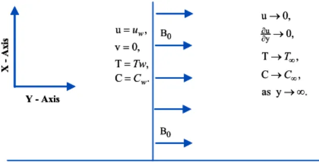
We consider Cartesian coordinate system in such a way that the x−axis is along the stretching surface and the y−axis is perpendicular to the x−axis. Magnetohydrodynamic boundary layer flow of a Jeffrey fluid is considered. A uniform magnetic field
0
B is applied parallel to the y−axis (see Figure 1). The induced magnetic field is neglected for small magnetic Reynolds number. Heat and mass transfer characteristics are taken into account in the presence of thermal radiation and thermophoresis effects. The uniform temperature of the surface Tw is larger than the ambient fluid temperature T∞.
Y - Axis
X
-Ax
is
B0 B0
u→0,
u y 0,
∂
∂ →
C→C∞, as y→ ∞. T→T∞, T=Tw,
C=Cw. u=uw, v=0,
Y - Axis
X
-Ax
is
B0 B0
u→0,
u y 0,
∂
∂ →
C→C∞, as y→ ∞. T→T∞, T=Tw,
C=Cw. u=uw, v=0,
Figure 1: Physical model
The species concentration at the surface Cw and ambient concentration C∞ are constants. Invoking the Rosseland approximation [24], the resulting equations take the following forms:
0,
∂ +∂ = ∂ ∂
u v
x y (1)
3 3
2 2 3
2 2 2
2 1 2 2 0 1
[ T( ) c( )],
u u u v u u u x y y u v
u u u u x y y
x y y x y B
u g T T C C
∗
∞ ∞
⎛ ⎛ ∂ + ∂ ⎞⎞
⎜ ⎜ ⎟⎟
∂ + ∂ = ν ⎜∂ + λ ⎜ ∂ ∂ ∂ ⎟⎟
⎜ ⎜ ∂ ∂ ∂ ∂ ⎟⎟
∂ ∂ + λ ∂ − +
⎜ ⎜ ∂ ∂ ∂ ∂ ∂ ⎟⎟
⎝ ⎠
⎝ ⎠
σ
− + β − + β −
ρ
(2)
2 3 2 2 2 2 2 2 0 16 3 , p p p
T T k T T T
u v
x y c y k y
u B
u
c y c
∞ ∗
∗ ∂ + ∂ = ∂ + σ ∂
∂ ∂ ρ ∂ ∂
⎛ ⎞
μ ∂ σ
+ ⎜ ⎟ + ρ ⎝∂ ⎠ ρ
(3)
2
2 ( ). ∂ + ∂ = ∂ − ∂
∂ ∂ ∂ ∂ T
C C C
u v D V C
x y y y (4)
Here ( , )u v are the velocity components along the
−
x and y−axes, λ1 and λ2 are the ratio of relaxation/retardation times and retardation time, respectively, ν the dynamic viscosity, ρ the density of the fluid, σ∗ the electrical conductivity, g the gravitational acceleration, βT and βc the thermal expansion coefficients, T the temperature, cp the specific heat, σ the Stefan-Boltzmann constant, k∗
the mean absorption coefficient, D the diffusion coefficient and VT the thermophoretic velocity.
, 0, ( ), ( ) at 0,
0, 0, ,
as . ∞ ∞ = = = = = = ∂ → → → → ∂ → ∞
w w w
u u ax v T T x C C x
y
u
u T T C C
y
y
(5)
where uw is the stretching velocity, Tw is the tem-perature at the wall, Cw is the concentration at the wall and T∞ and C∞ are the ambient fluid tempera-ture and concentration, respectively.
The term VT in Eq. (4) can be defined as follows:
1 , ν ∂ = − ∂ T r T V k
T y (6)
in which k1 is the thermophoretic coefficient and Tr
is the reference temperature. A thermophoretic pa-rameter τ is defined by the following relation:
1( − ∞). τ = − w
r
k T T
T (7)
The wall temperature and concentration fields are: , ,
∞ ∞
= + = +
w w
T T bx C C cx (8)
where ,a b and c are the positive constants. Through the following transformations:
( ), ( ),
( ) ∞ , ( ) ∞
∞ ∞
′
= η = − η η =
− −
θ η = φ η =
− −
w w
a
u axf v av f y
v
T T C C
T T C C
(9)
Equation (1) is automatically satisfied and Eqs. (2)-(4) are reduced as follows:
2 2 1
1 1
(1 )( ) ( )
(1 ) (1 ) ( ) 0,
′ ′′ ′′′′
′′′+ + λ ′′− + β − ′
− + λ + + λ γ θ + φ =
f ff f f ff
Mf N
(10)
2
2
4
(1 ) Pr[ ] Pr
3
Pr 0,
′′
′
′′ ′ ′
+ θ + θ − θ +
+ =
R f f Ecf
M Ecf
(11)
( ) ( ) 0,
′′ ′ ′ ′ ′ ′′
φ +Sc fφ − φf − τ φ θ − φθ =Sc (12)
0, 1, 1, 1 at 0,
f = f′= θ = φ = η =
(13) 0, 0, 0, 0 as .
f′→ f′′→ θ → φ → η → ∞
In the above expressions, β = λ2a is the Deborah number , M = σ∗B02/ρc the Hartmann number,
2
Re
γ = x x
Gr
the local buoyancy parameter,
3 2 2 2 2
( ) /
/ ∞
β − ν
=
ν
T w x
w
g T T x
Gr
u x the local Grashof number,
( ) ( ) ∞ ∞ β − =
βcT ww−
C C
N
T T the constant dimensionless
concen-tration buoyancy parameter, Pr=μcp
k the Prandtl
number,
3
4 ∗ ∞ ∗ σ = T R
k k the radiation parameter, 2 ( ∞) = − w p w u Ec
c T T the Eckert number and ν = Sc
D
the Schmidt number.
The skin friction coefficient, local Nusselt number and local Sherwood number are transformed to the following:
(
)
1/2 1/2 1 1/2 1Re (0) (0) , Re
1
(0), and Re (0). −
− ′′ ′′
= + β
+ λ
′ ′
= −θ = −φ
x f x x
x
C f f Nu
Sh
(14)
SERIES SOLUTIONS
The homotopic solutions for ,f θ and φ in a set of base functions:
{ηkexp(− ηn ), k≥0,n≥0} (15) can be written to the following expressions:
, 0 0
( ) exp( ),
∞ ∞
= =
η =
∑∑
k ηk − ηm m n
n k
f a n (16)
, 0 0
( ) exp( ),
∞ ∞
= =
θ η =
∑∑
k ηk − ηm m n
n k
, 0 0
( ) exp( ),
∞ ∞
= =
φ η =
∑∑
k ηk − ηm m n
n k
c n (18)
in which akm n, , bm nk, and cm nk, are the coefficients. Initial guesses and the auxiliary linear operators are
0 0
0
( ) (1 exp( ), ( ) exp( ), ( ) exp( ),
η = − −η θ η
= −η φ η = −η f
(19)
, θ , φ .
′′′ ′ ′′ ′′
= − = − = −
f
L f f L f f L f f (20) The operators in Eq. (19) satisfy the following properties:
1 2 3 4 5
6 7
( ) 0, ( )
0, ( ),
η −η η −η
θ η −η φ + + = + = + f
L C C e C e L C e C e
L C e C e
(21)
where Ci (i= −1 7) denote the arbitrary constants. The zeroth order deformation problems are expressible in the form
(
)
(
)
(
)
0
ˆ
1 ( ; ) ( )
ˆ( ; ), ( ; ), ( ; ) ,ˆ ˆ
− η − η =
η θ η φ η
=
f
f f
q L f q f
q N f q q q
(22)
(
)
(
)
(
)
0
ˆ
1 ( ; ) ( )
ˆ( ; ), ( ; ), ( ; ) ,ˆ ˆ θ
θ θ
− θ η − θ η =
θ η η φ η
=
q L q
q N q f q q
(23)
(
)
(
)
(
)
0
ˆ
1 ( ; ) ( )
ˆ( ; ), ( ; ), ( ; ) ,ˆ ˆ φ
φ φ
− φ η − φ η =
θ η η φ η
=
q L q
q N q f q q
(24)
ˆ(0; ) 0, (0; )ˆ 1, ( ; )ˆ 0, ( ; )ˆ 0,
ˆ(0; ) 1, ( ; )ˆ 0, (0; )ˆ 1 and ( ; )ˆ 0.
′ ′ ′′
= = ∞ = ∞ =
θ = θ ∞ = φ = φ ∞ =
f q f q f q f q
q q q q
(25)
Here q is the embedding parameter, =f , =θ and φ
= the non-zero auxiliary parameters and the nonlinear operators Nf , Nθ and Nφ are given by:
(
)
2 3 2 1 3 2 2 2 4 1 2 4 1ˆ( , ) ˆ( , ) ˆ( , )
ˆ ˆ ˆ ˆ
[ ( , ), ( ; ), ( ; )] (1 ) ( , )
ˆ( , ) ˆ( , ) ˆ( , )
ˆ ( , ) (1 )
ˆ ˆ
(1 ) ( ( , ) ( ; ) ,
⎛ ⎛ ⎞ ⎞
∂ η ⎜ ∂ η ∂ η ⎟
η θ η φ η = + + λ ⎜ η − ⎜⎜ ∂η ⎟⎟ ⎟
∂η ⎝ ∂η ⎝ ⎠ ⎠
⎛⎛∂ η ⎞ ∂ η ⎞ ∂ η
⎜ ⎟
+β⎜⎜⎜ ⎟⎟ − η ⎟− + λ ∂η
∂η ∂η
⎝ ⎠
⎝ ⎠
+ + λ γ θ η + φ η
f
f q f q f q
f q q q f q
f q f q f q
f q M
q N q
N
(26)
2 2
2 2
2 2
ˆ ˆ ˆ
4 ( , ) ( , ) ( , )
ˆ ˆ ˆ
[ ( , ), ( ; ), ( ; )] 1 Pr Pr
3
ˆ( , ) ˆ( , )
ˆ ˆ
Pr ( , ) Pr ( , ) ,
θ
⎛ ⎞ ⎛ ⎞
∂ θ η ∂ η ∂ η
⎛ ⎞
η θ η φ η =⎝⎜ + ⎟⎠ ∂η + ⎜⎜ ∂η ⎟⎟ + ⎜⎜ ∂η ⎟⎟
⎝ ⎠ ⎝ ⎠
∂ η ∂θ η
− θ η + η
∂η ∂η
q f q f q
f q q q R Ec M Ec
f q q
q f q
N (27) 2 2 2 2
ˆ( , ) ˆ( , ) ˆ( , )
ˆ ˆ ˆ ˆ ˆ
[ ( , ), ( ; ), ( ; )] ( , ) ( , )
ˆ( , ) ˆ( , ) ˆ( , )
ˆ( , ) .
φ
⎛ ⎞
∂ φ η ∂φ η ∂ η
η θ η φ η = + ⎜⎜ η ∂η − ∂η φ η ⎟⎟
∂η ⎝ ⎠
⎛∂θ η ∂φ η ∂ θ η ⎞ − τ⎜⎜ ∂η ∂η − φ η ⎟⎟
∂η
⎝ ⎠
q q f q
f q q q Sc f q q
q q q
Sc q
N
When q=0 and q=1, one has
0
ˆ( ;0)η = ( ); ( ;1)η ˆ η = ( ),η
f f f f (29)
0
ˆ( ;0) ( ); ( ;1)ˆ ( ),
θ η = θ η θ η = θ η (30)
0
ˆ( ;0) ( ); ( ;1)ˆ ( ).
φ η = φ η φ η = φ η (31)
Note that, when q increases from 0 to 1 , then ( , )η
f q , θ η( , )q and φ η( , )q approach f0( )η to ( )η
f , θ η0( ) to ( )θ η and φ η0( ) to ( ).φ η Accord-ing to Taylor's series, one has:
0
1
0
( , ) ( ) ( ) ,
1 ( ; )
( ) ,
! ∞
=
= η = η + ∑ η
∂ η η = ∂η m m m m m m q
f q f f q
f q
f
m
(32)
0
1
0
( , ) ( ) ( ) ,
1 ( ; )
( ) ,
! ∞
=
= θ η = θ η + ∑ θ η
∂ θ η θ η =
∂η m m m m m m q q q q m
(33)
0
1
0
( , ) ( ) ( ) ,
1 ( ; )
( ) .
! ∞
=
= φ η = φ η + ∑ φ η
∂ φ η φ η =
∂η m m m m m m q q q q m
(34)
The convergence of series (22)-(24) is closely associated with =f, =θ and =φ. The values of =f ,
θ
= and =φ are chosen such that the series (22)-(24) converge at q=1. Thus
0
1
( ) ( ) ( ), ∞
= η = η + ∑ m η
m
f f f (35)
0
1
( ) ( ) ( ), ∞
= θ η = θ η + ∑ θ ηm
m
(36)
0
1
( ) ( ) ( ). ∞
= φ η = φ η + ∑ φ ηm
m
(37)
The general solutions for fm, θm and φm in terms of special solutions fm∗, θ∗m and φ∗m are
1 2 3
( )η = ∗( )η + + η+ −η,
m m
f f C C e C e (38)
4 5
( ) ∗( ) η −η,
θ η = θ η +m m C e +C e (39)
6 7
( ) ∗( ) η −η.
φ η = φ η +m m C e +C e (40)
CONVERGENCE ANALYSIS AND DISCUSSION
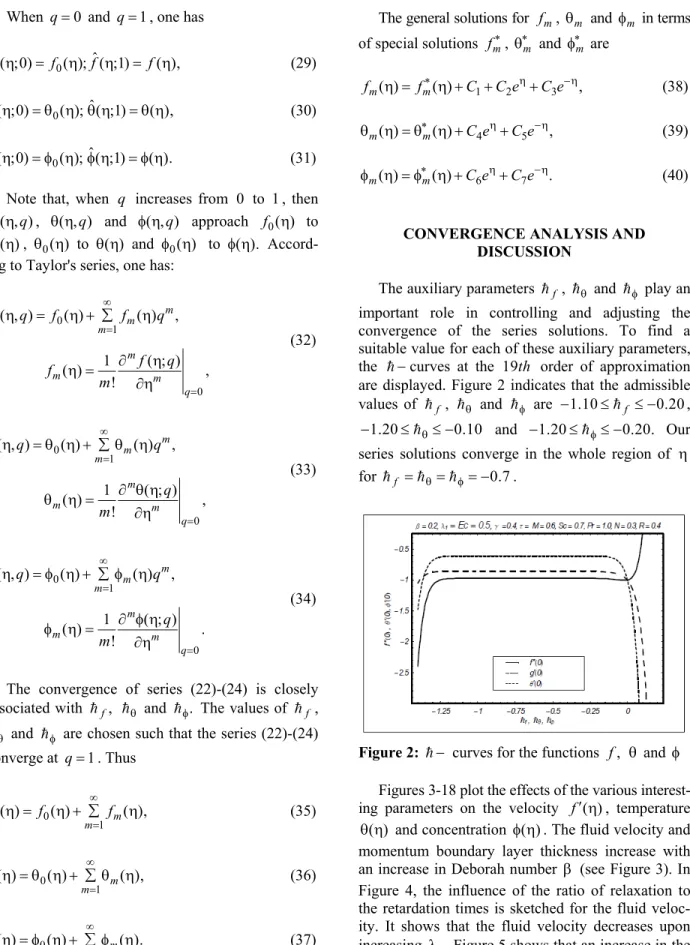
The auxiliary parameters =f , =θ and =φ play an important role in controlling and adjusting the convergence of the series solutions. To find a suitable value for each of these auxiliary parameters, the =−curves at the 19th order of approximation are displayed. Figure 2 indicates that the admissible values of =f , =θ and =φ are 1.10− ≤=f ≤ −0.20,
1.20 θ 0.10
− ≤= ≤ − and 1.20− ≤=φ≤ −0.20. Our series solutions converge in the whole region of η for 0.7=f ==θ==φ= − .
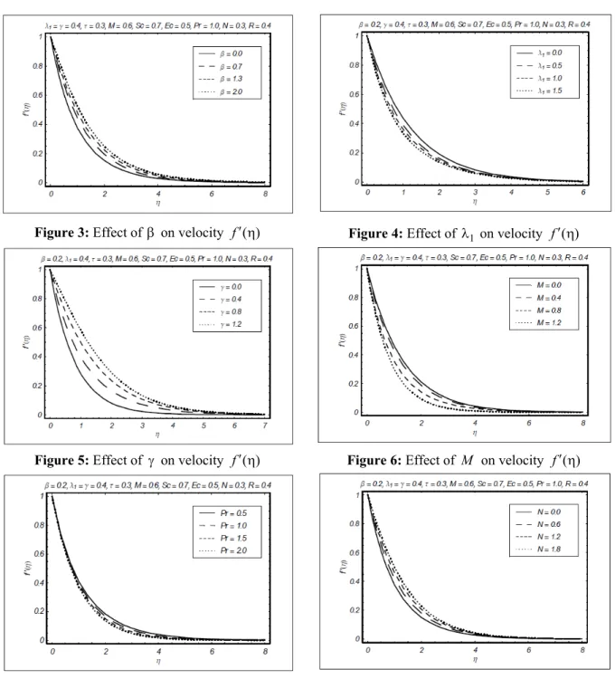
Figure 2: =− curves for the functions ,f θ and φ Figures 3-18 plot the effects of the various interest-ing parameters on the velocity f′ η( ), temperature
( )
local buoyancy parameter γ yields an increase in the velocity. In fact, the local buoyancy parameter depends on the buoyancy force and an increase in buoyancy force gives rise to the fluid velocity increase. An increase in Hartmann number M decreases the fluid velocity (see Figure 6). The Hartmann number is a consequence of the Lorentz force. Obviously an increase in the Lorentz force opposes the flow and thus the fluid velocity decreases. Figure 7 shows that
the velocity and momentum boundary layer thick-ness are decreasing functions of the Prandtl number
Pr . Figure 8 displays the effects of the ratio of buoyancy parameter N. The effects of the ratio of the buoyancy parameter are similar to that of γ in a qualitative way. The difference we noticed is that the fluid velocity increases more rapidly in the case of increasing local buoyancy parameter when compared with the ratio of the buoyancy parameter.
Figure 3: Effect of β on velocity f′ η( ) Figure 4: Effect of λ1 on velocity f′ η( )
Figure 5: Effect of γ on velocity f′ η( ) Figure 6: Effect of M on velocity f′ η( )
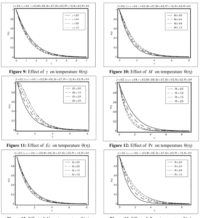
Effects of different parameters on the temperature are seen in Figures 9-14. Figure 9 depicts the effects of the local buoyancy parameter on the temperature field. The temperature field and thermal boundary layer thickness are reduced with an increase in γ. Figure 10 shows that the temperature increases when the Hartmann number is increased. In fact, large
M corresponds to lower permeability and hence the temperature and the thermal boundary layer thickness increase. Figures 11 and 12 illustrate the
influences of Eckert number Ec and Prandtl num-ber Pr on the temperature. It is observed from these figures that Ec and Pr have quite opposite effects on the velocity and the associated thermal boundary layer thickness. The temperature profile decreases more quickly for Ec in comparison to Pr . The ratio of the buoyancy parameter and the radiation parameter correspond to a decrease and an increase in the temperature, respectively (see Figures 13 and 14).
Figure 9: Effect of γ on temperature ( )θ η Figure 10: Effect of M on temperature ( )θ η
Figure 11: Effect of Ec on temperature ( )θ η Figure 12: Effect of Pr on temperature ( )θ η
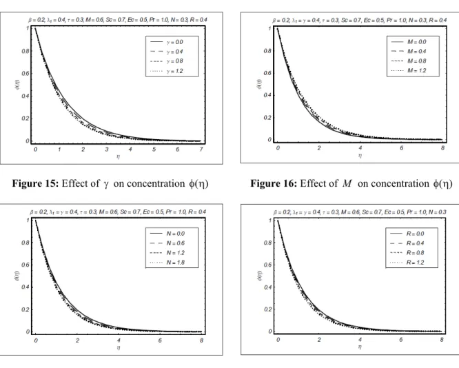
The effects of γ, M, N and R on concentration profile are seen through Figures 15-18. Figure 15 shows that the concentration and boundary layer thickness are decreasing functions of .γ It is found from Figure 16 that the Hartmann number increases the concentration profile and associated boundary layer thickness. The effects of N and R on ( )φ η are similar. Increases in N and R decrease the concentration and related boundary layer thickness (see Figures 17 and 18). It is worth mentioning here that the effects of M on the temperature are more pronounced when compared with the concentration. This same observation also holds for the influences of γ, N and R on the temperature and concentration.
Table 1 shows the convergence of the series solutions through computations of numerical values. This table indicates that our series solutions converge from the 20th-order of deformations for velocity and temperature and 25th-order of approximation for the
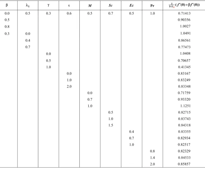
concentration. Table 2 includes the numerical values of the skin-friction coefficient for the different values of ,β λ1, ,τ M, Sc Sc, Ec and Pr when N =0.3 and R=0.4. The skin-friction coefficient increases with increasing ,β M, Sc and Pr . It decreases when
1,
λ γ and Ec are increased. Interestingly the varia-tion in the values of the skin-fricvaria-tion coefficient is very small with increasing thermophoretic parameter
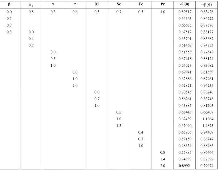
τ. Table 3 consists of the values of the local Nusselt and Sherwood numbers. The values of the local Nusselt and Sherwood numbers increase slowly in comparison to the increase in the values of the skin-friction coefficient when β increases. The increase in the values of the local Nusselt number is very small upon increasing τ, but the increase in the values of the local Sherwood number is large. A comparative study of Tables 2 and 3 shows that the values of the skin-friction coefficient and local Sherwood number are larger than the values of the local Nusselt number.
Figure 15: Effect of γ on concentration ( )φ η Figure 16: Effect of M on concentration ( )φ η
Table 1: Convergence of series solutions for different order of approximations when β= 0.2, γ =0.4, 0.6,
M
τ = = Sc=0.7, λ =Ec=0.5, Pr=1.0, N =0.3, R=0.4 and =f ==θ==φ= −0.7.
Order of approximations −f′′(0) −θ′(0) −φ(0)
1 1.03150 0.66750 0.89500
5 0.99364 0.61878 0.85224
10 0.99306 0.61970 0.84720
20 0.99305 0.61974 0.84646
25 0.99305 0.61974 0.84643
30 0.99305 0.61974 0.84643
35 0.99305 0.61974 0.84643
Table 2: Numericalvalues of skin-friction coefficientfor different values of β, λ1, τ,, M, Sc, Ec and Pr when N= 0.3 and R= 0.4.
β λ1 γ τ M Sc Ec Pr 1 ′′ ′′
1
1+λ (f (0)+ βf (0))
0.0 0.5 0.3 0.6 0.5 0.7 0.5 1.0 0.71413
0.5 0.90356
0.8 1.0027
0.3 0.0 1.0491
0.4 0.86561
0.7 0.77473
0.0 1.0408
0.5 0.70657
1.0 0.41345
0.0 0.83167
1.0 0.83249
2.0 0.83348
0.0 0.71759
0.7 0.93320
1.0 1.1251
0.5 0.82715
1.0 0.83743
1.5 0.84318
0.4 0.83355
0.7 0.82934
1.0 0.82517
0.8 0.82329
1.4 0.84533
Table 3: Numerical values of local Nusselt number -θ′(0) and local Sherwood number −φ′
( )
0 for different values of β, λ1, τ, M, Sc, Ec and Pr when N=0.3 and R=0.4.1
λ τ M Sc Ec Pr -θ′(0) −φ′( )0
0.0 0.5 0.3 0.6 0.5 0.7 0.5 1.0 0.59817 0.83428
0.5 0.64563 0.86222
0.8 0.66635 0.87576
0.3 0.0 0.67517 0.88177
0.4 0.63701 0.85682
0.7 0.61469 0.84353
0.0 0.51553 0.77548
0.5 0.67418 0.88124
1.0 0.74023 0.93082
0.0 0.62941 0.81539
1.0 0.62886 0.87961
2.0 0.62821 0.96235
0.0 0.70545 0.86946
0.7 0.56261 0.83748
1.0 0.43885 0.81203
0.5 0.63443 0.66407
1.0 0.62439 1.1064
1.5 0.62040 1.4825
0.4 0.65805 0.84409
0.7 0.57159 0.86747
1.0 0.48634 0.88986
0.8 0.55885 0.86466
1.4 0.74998 0.82693
2.0 0.8992 0.79074
CLOSING REMARKS
In this study we discussed the effects of thermal radiation, Joule heating and thermophoresis in stretched flow of a Jeffrey fluid. The main observations are as follows:
Effects of β and λ1 on the fluid velocity are quite
opposite.
An increase in the ratio of the buoyancy parame-ter N corresponds to an increase in f′ η( ).
The fluid temperature rises with an increase in Eckert number Ec.
Effects of the ratio of the buoyancy parameter and radiation parameter are qualitatively similar.
Variations in temperature are more pronounced than those in concentration when M increases.
The increase in the values of the skin-friction coefficient and the local Nusselt number is very small in comparison to the increase in the local
Sherwood number when τ increases.
Numerical values of the local Nusselt number increase and the values of the local Sherwood num-ber decrease with increasing Prandtl numnum-ber Pr .
ACKNOWLEDGMENTS
The research of Alsaedi was partially supported by the Deanship of Scientific Research (DSR), King Abdulaziz University, Jeddah, Saudi Arabia. We are also thankful to the reviewer for his/her useful suggestions.
REFERENCES
steady MHD combined free-forced convective heat and mass transfer flow over a semi-infinite permeable inclined plate in the presence of thermal radiation. Int. J. Thermal Sci., 47, p. 758 (2008).
Aziz, R. C., Hashim, I. and Abbasbandy, S., Effects of thermocapillarity and thermal radiation on flow and heat transfer in a thin liquid film on an unsteady stretching sheet. Math. Problems Eng., DOI:10.1155/2012/127320.
Bhattacharyya, K., Mukhopadhyay, S. and Layek, G. C., Slip effects on an unsteady boundary layer stagnation-point flow and heat transfer towards a stretching sheet. Chin. Phy. Lett., 28, p. 09470 (2001).
Goren, S. L., Thermophoresis of aerosol particles in laminar boundary layer on flat plate. J. Colloid Interf. Sci., 61, p. 77 (1977).
Haitao, Q. and Mingyu, X., Unsteady flow of viscoelastic fluid with fractional Maxwell model in a channel. Mech. Research Commun., 34, p. 210 (2007).
Hayat, T. and Alsaedi, A., On thermal radiation and Joule heating effects in MHD flow of an Oldroyd-B fluid with thermophoresis. Arab. J. Sci. Eng., 36, p. 1113 (2011).
Hayat, T. and Qasim, M., Influence of thermal radiation and Joule heating on MHD flow of a Maxwell fluid in the presence of thermophoresis. Int. J. Heat Mass Transfer, 53, p. 4780 (2010). Hayat, T., Qasim, M. and Abbas, Z., Radiation and
mass transfer effects on the magnetohydrodynamic unsteady flow induced by a stretching sheet. Z Naturforsch A. 64, p. 231 (2010).
Hayat, T., Shehzad, S. A. and Qasim, M., Mixed convection flow of a micropolar fluid with radia-tion and chemical reacradia-tion. Int. J. Num. Methods Fluids, 67, p. 1418 (2011).
Hayat, T., Shehzad, S. A., Qasim, M. and Obaidat, S., Flow of a second grade fluid with convective boundary conditions. Thermal Sci., 15, p. S253 (2011).
Hayat, T., Shehzad, S. A., Qasim, M. and Obaidat, S., Radiative flow of Jeffery fluid in a porous medium with power law heat flux and heat source. Nuclear Eng. Design, 243, p. 15 (2012). Hayat, T., Shehzad, S. A., Qasim, M. and Obaidat,
S., Steady flow of Maxwell fluid with convective boundary conditions. Z. Naturforsch 66a, p. 417 (2011).
Hayat, T., Shehzad, S. A., Qasim, M. and Obaidat, S., Thermal radiation effects on the mixed convection stagnation-point flow in a Jeffery fluid. Z. Naturforsch 66a, p. 606 (2011).
Hinds, W. C., Aerosol Technology: Properties, Behavior, and Measurement of Airborne Particles. John Wiley and Sons, New York, (1982).
Jamil, M. and Fetecau, C., Helical flows of Maxwell fluid between coaxial cylinders with given shear stresses on the boundary. Nonlinear Analysis: Real World Appl., 11, p. 4302 (2010).
Jamil, M. and Fetecau, C., Some exact solutions for rotating flows of a generalized Burgers' fluid in cylindrical domains. J. Non-Newtonian Fluid Mech., 165, p. 1700 (2010).
Jamil, M., Khan, N. A. and Zafar, A. A., Translational flows of an Oldroyd-B fluid with fractional derivatives. Comput. Math. Appl., 62, p. 1540 (2011).
Kothandapani, M. and Srinivas, S., Peristaltic transport of a Jeffrey fluid under the effect of magnetic field in an asymmetric channel. Int. J. Non-Linear Mech 43, p. 915 (2008).
Liao, S. J., Beyond Perturbation: Introduction to Homotopy Analysis Method. Chapman and Hall, CRC Press, Boca Raton (2003).
Makinde, O. D. and Aziz, A., Boundary layer flow of a nano fluid past a stretching sheet with con-vective boundary conditions. Int. J. Thermal. Sci., 50, p. 1326 (2011).
Nadeem, S. and Akbar, N. S., Peristaltic flow of a Jeffrey fluid with variable viscosity in an asym-metric channel. Zeitschrift fur Naturforschung A 64, p. 713 (2010).
Nadeem, S., Zaheer, S. and Fang, T., Effects of thermal radiation on the boundary layer flow of a Jeffery fluid over an exponentially stretching surface. Numer. Algor., 57, p. 187 (2011).
Noor, N. F. M., Abbasbandy, S. and Hashim, I., Heat and mass transfer of thermophoretic MHD flow over an inclined radiate isothermal permeable surface in the presence of heat source/sink. Int. J. Heat Mass Transfer, 55, 2122 (2012).
Rashidi, M. M. and Erfani, E., A new analytical study of MHD stagnation-point flow in porous media with heat transfer. Comput. Fluids, 40, p. 172 (2011).
Rashidi, M. M. and Pour, S. A. M., Analytic ap-proximate solutions for unsteady boundary-layer flow and heat transfer due to a stretching sheet by homotopy analysis method. Nonlinear Analysis: Modelling and Control, 15, p. 83 (2010).
Rashidi, M. M., Pour, S. A. M. and Abbasbandy, S., Analytic approximate solutions for heat transfer of a micropolar fluid through a porous medium with radiation. Commun. Nonlinear Sci. Numer. Simulat., 16, p. 1874 (2011).
Analytic approximate solutions for heat transfer of a micropolar fluid through a porous medium with radiation. Commun. Nonlinear Sci. Numer. Simulat., 16, p. 1874 (2011).
Sahoo, B. and Poncet, S., Flow and heat transfer of a third grade fluid past an exponentially stretching sheet with partial slip boundary condition. Int. J. Heat Mass Transfer, 54, p. 5010 (2011).
Tasai, C. J., Lin, J. S., Shankar, I., Aggarwal, G. and Chen, D. R., Thermophoretic deposition of particles in laminar and turbulent tube flows. Aerosol Sci. Tech., 38, p. 131 (2004).
Vosughi, H., Shivanian, E. and Abbasbandy, S., A new analytical technique to solve Volterra's integral equations. Math. Methods Appl. Sci. 34, p. 1243 (2011).
Vyas, P. and Rai, A., Radiative flow with variable thermal conductivity over a non-isothermal stretch-ing sheet in a porous medium. Int. J. Contemp. Math. Sciences, 5, p. 2685 (2010).
Wang, S. and Tan, W. C., Stability analysis of soret-driven double-diffusive convection of Maxwell fluid in a porous medium. Int. J. Heat Fluid Flow 32, p. 88 (2011).
Yao, B., Approximate analytical solution to the Falkner-Skan wedge flow with the permeable wall of uniform suction, Commun. Nonlinear Sci. Numer. Simulat. 14, p. 3320 (2009).