Homogeneous-heterogeneous reactions in peristaltic flow with convective conditions.

This article addresses the effects of homogeneous-heterogeneous reactions in peristaltic transport of Carreau fluid in a channel with wall properties. Mathematical modelling and analysis have been carried out in the presence of Hall current. The channel walls satisfy the more realistic convective conditions. The governing partial differential equations along with long wavelength and low Reynolds number considerations are solved. The results of temperature and heat transfer coefficient are analyzed for various parameters of interest.

Introduction

In the last few decades, the peristaltic motion of non-Newtonian fluids is a topic of major contemporary interest both in engineering and biological applications. To be more specific, such motion occurs in powder technology, fluidization, chyme movement in the gastrointestinal tract, vasomotion of small blood vessels, locomotion of worms, gliding motility of bacteria, passage of urine from kidney to bladder, reproductive tracts, corrosive and sanitary fluids transport, roller, finger and hose pumps and blood pump through heart lung machine. There is no doubt that viscoelasticity has key role mostly in all the aforementioned applications. Viscoelastic materials are non-Newtonian and possess both the viscous and elastic properties. Most of the biological liquids such as blood at low shear rate, chyme, food bolus etc. are viscoelastic in nature. Another aspect which has yet not been properly addressed is the interaction of rheological characteristics of fluids in peristalsis with convective effects. The significance of convective heat exchange with peristalsis cannot be under estimated for instance in translocation of water in tall trees, dynamic of lakes, solar ponds, lubrication and drying technologies, diffusion of nutrients out of blood, oxygenation, hemodialysis and nuclear reactors. The heat and mass transfer effects in such processes have prominent role. OPEN ACCESS

Citation:Hayat T, Tanveer A, Yasmin H, Alsaedi A (2014) Homogeneous-Heterogeneous Reactions in Peristaltic Flow with Convective Conditions. PLoS ONE 9(12): e113851. doi:10. 1371/journal.pone.0113851

Editor:Sanjoy Bhattacharya, Bascom Palmer Eye Institute, University of Miami School of Medicine, United States of America

Received:July 11, 2014

Accepted:November 2, 2014

Published:December 2, 2014

Copyright:ß2014 Hayat et al. This is an open-access article distributed under the terms of the

Creative Commons Attribution License, which permits unrestricted use, distribution, and repro-duction in any medium, provided the original author and source are credited.

Data Availability:The authors confirm that all data underlying the findings are fully available without restriction. All relevant data are within the paper.

Funding:The authors have no support or funding to report.

aspects including heat/mass transfer, MHD etc. Few representative attempts in this direction can be mentioned through the recent researchers [1–13] and several studies therein.

To our knowledge, no study has been undertaken yet to discuss the effects of homogeneous-heterogeneous reactions in peristaltic flows of non-Newtonian fluids. Even such study is yet not presented for the viscous fluid. However such consideration is quite important because many chemically reacting systems involve both homogeneous and heterogeneous reactions, with examples occurring in combustion, biochemical systems, catalysis, crops damaging through freezing, cooling towers, fog dispersion, hydrometallurgical processes etc. Hence the main objective of present investigation is to model and analyze the peristalsis of Carreau fluid in a compliant wall channel with convective conditions and homogeneous-heterogeneous reactions. Effects of Hall current and viscous dissipation are also considered. The resulting mathematical systems are solved and examined in the case of long wavelength and small Reynolds number. This article is structured as follows. Section two consists of mathematical modelling and solution expressions up to first order. The behaviors of sundry variables on the temperature, heat transfer coefficient and concentration are discussed graphically in section three. Main results of present study are also included in this section.

Mathematical Formulation

Consider the peristaltic transport of an incompressible Carreau fluid in two-dimensional compliant wall channel. The channel walls satisfy the convective conditions. The Cartesian coordinatesxandyare considered along and transverse to the direction of fluid flow respectively. The flow is generated by the peristaltic wave of speed c travelling along the channel walls. The Hall effects are also considered in the flow analysis. Further we consider the flow in the presence of a simple homogeneous and heterogeneous reaction model. There are two chemical species A and Bwith concentrations a andb respectively. The physical model of the wall surface can be analyzed by the expression:

y~+g(x,t)~_dz_asin2

p

whereJrepresents the current density,sthe electrical conductivity,Vthe velocity field, ethe electric charge and^n the number density of electrons. Also the effects of electric field are considered absent i.e. E~₀:

IfV~½_{u,u,0is the velocity with componentsu and uin thex andydirections} respectively then from Eqs. (2) and (3) we have

J|B0~ {_sB2₀ 1zm2 u

{_mu

ð Þ,ðuz_muÞ,₀

½ , _ð4_Þ

where m~sB0

en^ serves as the Hall parameter. The reaction model is considered in the form [14–16]:

Az2_B?3B, rate~_kcab2_,

while on the catalyst surface we have the single, isothermal, first order chemical reaction.

A?B, rate~_ksa,

in which kc andks are the rate constants. Both reaction processes are assumed

isothermal.

The corresponding flow equations are as follows:

L_u

L_xz

L_u

L_y~0, ð5Þ

rdu dt~{

L_p

L_xz

L_Rxx

L_x z

L_Rxy

L_y {

sB20

1z_m2ðu{muÞ, ð6Þ

rdu dt~{

L_p

L_yz

L_Ryx

L_x z

L_Ryy

L_y {

sB2 0 1z_m2 u

z_mu

ð Þ, _ð7_Þ

rcp

dT dt ~k

L2_T

L_x2z

L2_T L_y2

z_Rxx

L_u L_xzRxy

L_u

L_xzRyx L_u L_yzRyy

L_u

Hereg? is the infinite shear-rate viscosity,g0 the zero shear-rate viscosity,C the time constant andnthe dimensionless form of power law index(nv1). Alsoc_ is defined as follows:

_ c~

ffiffiffiffiffiffiffiffiffiffiffiffiffiffiffiffiffiffiffiffiffiffiffiffiffiffiffi

1 2

X

i X

j

_ c_ijc__ji

s

~

ffiffiffiffiffiffiffiffi

1 2P

r

, _ð12_Þ

where P_{denotes the second invariant strain tensor defined by}

P~_tr½+Vz₍+V)t2 and c_~+Vz₍+V)t: Here we consider the case for which g?~0 and Cc_v1:Therefore the extra stress tensor takes the form

R~g₀ 1z(C_{c_)}2n

{1 2

_

c: _ð13_Þ

It is worth mentioning that the above model reduces to viscous model forn~_1or

C~0: The component forms of extra stress tensor are

Rxx ~2m0½1z n{1

2 (Cc_) 2

L_Lu

x, ð14Þ

Rxy~m0½1z n{1

2 (Cc_) 2

(Lu

L_yz

L_u

L_x)~Ryx, ð15Þ

Ryy~2m0½1z n{1

2 (Cc_) 2

L_Lu

y: ð16Þ

In above equations d

dt is the material time derivative,r the density of fluid,m0 the fluid viscosity, n the kinematic viscosity, T the fluid temperature,C the concentration of fluid, T0 and T1 the temperatures at the lower and upper walls respectively, K the measure of the strength of homogeneous reaction, DA andDB

the diffusion coefficients for homogeneous and heterogeneous reactions, cp the

The exchange of heat at the walls is given by

kLT

L_y ~ {h1(T{T1), aty~g,

kLT

L_y ~ {h2(T0{T), aty~{g:

ð17_Þ

Hereh1 and h2 indicate the heat transfer coefficients at the upper and lower walls respectively.

The no-slip condition at the boundary wall is represented by the following expressions

u~₀,u~+g_t aty~+g: _ð18_Þ

The compliant wall properties are described through the expression

{t

L3

L_x3zm

1

L3

L_xL_t2zd 0 L2

L_tL_x

g~

{_rdu dtz

L_Rxx

L_x z

L_Rxy

L_y {

sB2 0 1z_m2 u

{_mu

ð Þ at y~+g,

ð19_Þ

in whichtis the elastic tension in the membrane,m1the mass per unit area andd’ the coefficient of viscous damping. The mass conditions under the homogeneous and heterogeneous reactions are given through the following expressions:

DA

L_a

L_y~ksa, at y~+g, ð20Þ

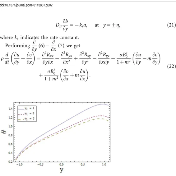
Figure 1. Plot of temperaturehfor wall parametersE1,E2,E3,withE~0:1,t~0:01,x~0:2,ª1~4,ª2~6,

Br~1,m1~2,n~0:4,We~0:4andm~0:04

DB

L_b

L_y~{ksa, at y~+g, ð21Þ

where ks indicates the rate constant.

Performing L

L_y (6){ L

L_x (7) we get

r d dt

L_u

L_y{

L_u

L_x

~

L2_Rxx L_yL_x{

L2_Ryx

L_x2 z

L2_Rxy

L_y2 {

L2_Ryy L_xL_y{

sB2 0 1z_m2

L_u

L_y{m

L_u

L_y

z sB 2 0 1z_m2

L_u

L_xzm

L_u L_x

:

ð22_Þ

Figure 2. Plot of temperaturehfor Brinkman numberBrwithE~0:1,_t~0:01,_x~0:2,ª1~4,ª2~6,E1~0:4,

E2~0:2,E3~0:3,m1~2,n~0:4,We~0:4andm~0:04

doi:10.1371/journal.pone.0113851.g002

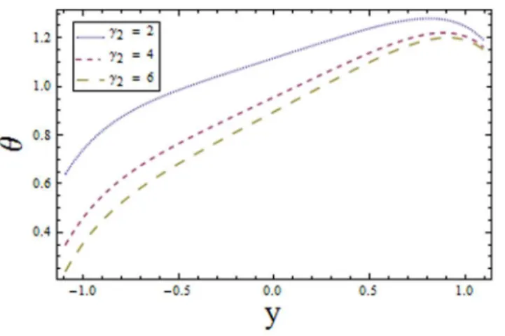
Figure 3. Plot of temperaturehfor Biot numberª1withE~0:1,t~0:01,x~0:2,Br~1,ª2~6,E1~0:4,

E2~0:2,E3~0:3,m1~2,n~0:4,We~0:4andm~0:04

Introducing the stream functionyðx,y,tÞand defining the following dimensionless variables:

u~

L_y

L_y, u~{

L_y

L_x,

y~y cd,x

_~x l,y

_~y d,t

_~ct l,g

_~g d,h~

T{_T0 T1{T0

,bc_{_}~d cc_,j

_~DB

DA ,

g~ a a0

,h~ b a0

,R_xx~ l

m₀cRxx,R

xy~

d

m₀cRxy,R

yx~

d m₀cRyx,R

yy~

d

m₀cRyy: ð23Þ

Eqs. (8), (9) and (22) yield

dRe d dt

L2_y

L_y2zd 2L2y

L_x2

~d2

L2_Rxx L_yL_x {d

2L 2

Ryx

L_x2 z

L2_Rxy

L_y2 zd

L2_Ryy L_xL_y

{ m 2 1 1z_m2

L2_y

L_y2zd 2L2y

L_x2z2md

L2_y

L_xL_y

,

ð24_Þ

dPr Redh dt~

d2L 2

h

L_x2z

L2_h

L_y2zBr d

2 Rxx

L2_y

L_y2{d 2

Rxy

L2_y

L_x2zRyx

L2_y

L_y2 {d 3

Ryy

L2_y

L_xL_y

,

ð25_Þ

Reddg dt~ 1 Sc d 2L 2 g

L_x2z

L2_g L_y2

{_Kgh2, ð₂₆Þ

Figure 4. Plot of temperaturehfor Biot numberª2withE~0:1,_t~0:01,_x~0:2,ª1~4,Br~1E1~0:4,

E2~0:2,E3~0:3,m1~2,n~0:4,We~0:4andm~0:04:

Reddh dt~

j Sc d

2L 2

h

L_x2z

L2_h L_y2

z_Kgh2, ð₂₇Þ

with the dimensionless conditions

g~1zEsin 2pð_x{tÞ, ð28Þ

L_h

L_yzc1(h{1)~0 aty~g, L_h

L_y{c2h~0 aty~{g, ð29Þ

L_g

L_y{Mg~0 aty~+g, ð30Þ

jLh

L_yzMh~0 aty~+g, ð31Þ

y_y~_{0 aty}~+g, _ð32_Þ

E1

L3

L_x3zE2

L3

L_xL_t2zE3

L2

L_xL_t

g~{_Redd dt(

L_y

L_y)zd

2 L

L_xRxxz L

L_yRxy

{ m 2 1 1zm2

L_y

L_yzmd

L_y

L_x

aty~+g: _ð33_Þ

Figure 5. Plot of temperaturehfor Hall parametermwithE~0:1,_t~0:01,_x~0:2,ª1~4,ª2~6,E1~0:4,

E2~0:2,E3~0:3,m1~2,n~0:4,We~0:4andBr~1:

Also Eqs. (14–16) become

Rxx~ 2(1z

n{₁ 2 We

2_b _

c2)y_xy, _ð34_Þ

Rxy~ Ryx~2(1z

n{1 2 We

2_b _

c2)(y_yy{_d2_y

xx), ð35Þ

Ryy~ {2d(1z

n{₁ 2 We

2_b _

c2)y_xy: _ð36_Þ

In above equations asterisks have been omitted for simplicity. Hered is the dimensionless wave number, the Reynolds numberRe, the Prandtl numberPr, the

Figure 6. Plot of temperaturehfor Hartman numberm1withE~0:1,_t~0:01,_x~0:2,ª1~4,ª2~6,E1~0:4,

E2~0:2,E3~0:3,Br~1,n~0:4,We~0:4andm~0:04:

doi:10.1371/journal.pone.0113851.g006

Figure 7. Plot of temperaturehfor Weissenberg numberWewithE~0:1,t~0:01,x~0:2,ª1~4,ª2~6, E1~0:4,E2~0:2,E3~0:3,m1~2,n~0:4,Br~1andm~0:04:

amplitude ratio E, the chemical reaction parameter c, the Hartman number m₁, the non-dimensional elasticity parameters E1,E2,E3, the Schmidt numberSc, the Eckert numberE,the Brinkman numberBr, the heat transfer Biot numbersc₁,c₂,

the Weissenberg number We, the ratio of diffusion coefficient j,the strength measuring parameters K and M (for homogeneous and heterogeneous reaction respectively) and^_c(non-dimensional form ofc) are given through the following_ variables:

d~ d l,Re~

cd n ,Pr~

mcp

k ,E~ a d,We~

C_c

d ,E~ c2

(T1{T0)cp ,

Sc~ m0 rDA

,E1~{ td3 l3m₀c,E2~

m1cd3 l3m₀ ,E3~

d3d0

ml2 ,Br~EPr,

bc_{_} ~

ffiffiffiffiffiffiffiffiffiffiffiffiffiffiffiffiffiffiffiffiffiffiffiffiffiffiffiffiffiffiffiffiffiffiffiffiffiffiffiffiffiffiffiffiffiffiffiffiffiffiffiffiffiffiffiffiffiffiffiffiffiffi

4d2 L 2

y

L_xL_y

2

z

L2_y

L_y2{d 2L

2 y

L_x2

s

,c1~ h1d

k ,c2~ h2d

k ,

m21 ~

sB2₀d2 m₀ ,j~

DB

DA

,K~kca 2 0d

2

n ,M~ ksd

DA :

ð37_Þ

We now employ the approximations of long wavelength and low Reynolds number [17–23] and equality of diffusion coefficients DA and DB i.e. j~1:The

assumption j~1 leads to the following relation:

g(g)z_h(g)~_1, ð₃₈Þ

and we obtain the following set of equations

Figure 8. Plot of temperaturehfor power law indexnwithE~0:1,t~0:01,x~0:2,ª1~4,ª2~6,E1~0:4,

E2~0:2,E3~0:3,m1~2,We~0:4,Br~1andm~0:04:

L4_y

L_y4z

3

2(n{1)We 2L

4 y

L_y4

L2_y

L_y2

2

z3(n{1)We2

L3_y

L_y3

2

L2_y

L_y2{

m21 1z_m2

L2_y

L_y2 ~0,

ð39_Þ

L2_h

L_y2zBr

L2_y

L_y2

2

1zn {₁

2 We 2 L

2 y

L_y2

2!

~_0, ð₄₀Þ

1 Sc

L2_g

L_y2{Kg(1{g) 2_~

0, _ð41_Þ

Figure 9. Plot of heat transfer coefficientZ for wall parametersE1,E2,E3,withE~0:1,_t~0:01,ª1~4,

ª2~6,m1~2,We~0:4,n~0:4,Br~1andm~0:04:

doi:10.1371/journal.pone.0113851.g009

Figure 10. Plot of heat transfer coefficientZfor Brinkman numberBrwithE~0:1,t~0:01,ª1~4,ª2~6,

L_y

L_y ~ 0 at y~+g, ð42Þ

L_h

L_yzc1ðh{1Þ ~ 0, at y~g,

L_h

L_y{c2h ~ 0, at y~{g,

ð43_Þ

L_g

L_y{Mg ~ 0,at y~+g, ð44Þ

E1

L3

L_x3zE2

L3

L_xL_t2zE3

L2

L_xL_t

g ~

L3_y

L_y3z

3

2(n{1)We 2 L

2 y

L_y2

2

L3_y

L_y3

{ m 2 1 1z_m2

L_y

L_y aty ~ +g:

ð45_Þ

2.1 Method of solution

It is seen from Eqs. (39) and (41) that these Eqs. are non-linear and involve Weissenberg number We and homogeneous reaction parameter K respectively. Therefore the problem at hand cannot be solved exactly, but can be linearized about "small" parameter to the mathematical description of the exactly solvable problem. The technique is referred as perturbation. Perturbation method

represent a very powerful tool in modern mathematical physics and, in particular, in fluid dynamics and leads to a series solution of resulting system of equations having small paramter. Therefore we have applied this method to form the series

Figure 11. Plot of heat transfer coefficientZfor Biot numberª1withE~0:1,_t~0:01,_Br~1,ª2~6,E1~0:4,

E2~0:2,E3~0:3,m1~2,n~0:4,We~0:4andm~0:04:

solutions for stream function y, temperatureh and concentration g corre-sponding to the involved non-linear quantities (WeandK). For this we write the flow quantities in the forms:

y~_y0z_We2_y1z_{O We} 4_,

h~_h0z_We2_h1z_{O We} 4_,

g~_g0z_Kg1z_{O K} 2_,

Z~_Z0z_We2_Z1z_O(We4):

2.2 Zeroth order system and its solution

The zeroth order system is given by

L4_y0

L_y4 {

m21 1z_m2

L2_y0

L_y2 ~0, ð46Þ

L2_h0

L_y2 zBr

L2_y0

L_y2

2

~_{0, ð47Þ}

1 Sc

L2_g0

L_y2 ~0, ð48Þ

L_y0

L_y ~0, aty~+g, ð49Þ

Figure 12. Plot of heat transfer coefficientZfor Biot numberª2withE~0:1,_t~0:01,ª1~4,Br~1,E1~0:4,

E2~0:2,E3~0:3,m1~2,n~0:4,We~0:4andm~0:04:

L_h0

L_y zc1(h0{1)~0 at y~g,

L_h0

L_y {c2h0~0 at y~{g, ð50Þ

L_g0

L_y {Mg0~0, aty~+g, ð51Þ

Figure 13. Plot of heat transfer coefficientZfor Hall parametermwithE~0:1,_t~0:01,ª1~4,ª2~6,

E1~0:4,E2~0:2,E3~0:3,m1~2,n~0:4,We~0:4andBr~1:

doi:10.1371/journal.pone.0113851.g013

Figure 14. Plot of heat transfer coefficientZfor Hartman numberm1withE~0:1,t~0:01,ª1~4,ª2~6,

E1~0:4,E2~0:2,E3~0:3,Br~1,n~0:4,We~0:4andm~0:04:

E1

L3

L_x3zE2

L3

L_xL_t2zE3

L2

L_xL_t

g~

L3_y0

L_y3 {

m21 1zm2

L_y0

L_y aty~+g: ð52Þ

The solutions of Eqs. (46–48) subject to the boundary conditions (49–52) are

y₀~A₂(pffiffiffiffiHy{sech(pHffiffiffiffig)sinh(pffiffiffiffiHy)), ð53Þ

h0~{L4z 4L5

H y

2_{(L4c2{L2) 1z_c2g y

{2L5cosh(2

ffiffiffiffi

H

p

y)

H2 , ð54Þ

g0~B1zB2y, ð55Þ

Z0~gxh0y(g),

~_gx½

{_4L5({₂pffiffiffiffi_Hgz_sinh(2pffiffiffiffi_Hg))

H3=2 {

L4c2 1zc₂g

{2L5(

{_2Hg(2z_c2g)z_c2cosh(2p_Hffiffiffiffi_g)z₂pffiffiffiffi_Hsinh(2pffiffiffiffi_Hg)) H2_(1zc

2g)

:

ð56_Þ

2.3 First order system and its solution

At this order we have

L4_y1

L_y4 z

3 2(n{1)

L4_y0

L_y4

L2_y0

L_y2

2

z_3(n{₁₎

L3_y0

L_y3

2

L2_y0

L_y2 {

m2 1 1z_m2

L2_y1

L_y2 ~0, ð57Þ

Figure 15. Plot of heat transfer coefficientZfor Weissenberg numberWewithE~0:1,_t~0:01,ª1~4,

ª2~6,E1~0:4,E2~0:2,E3~0:3,m1~2,n~0:4,Br~1andm~0:04:

L2_h1

L_y2 z2Br

L2_y0

L_y2

L2_y1

L_y2 z

Br(n{₁₎ 2

L2_y0

L_y2

4

~0, ð58Þ

1 Sc

L2_g1

L_y2 {g0(1{g0) 2_~

0, _ð59_Þ

L_y1

L_y ~0,aty~+g, ð60Þ

L_h1

L_y zc1h1~0 at y~g,

L_h1

L_y {c2h1~0 at y~{g, ð61Þ

L_g1

L_y {Mg1~0, aty~+g, ð62Þ

L3_y1

L_y3 z

3 2(n{1)

L3_y0

L_y3

L2_y0

L_y2

2

{ m 2 1 1z_m2

L_y1

L_y ~0 aty~+g: ð63Þ

Solving Eqs. (57–59) and then applying the corresponding boundary conditions we get the solutions in the forms given below:

Figure 16. Plot of heat transfer coefficientZfor power law indexnwithE~0:1,_t~0:01,ª1~4,ª2~6,

E1~0:4,E2~0:2,E3~0:3,m1~2,Br~1,We~0:4andm~0:04:

y₁~A₃A₄exp({pffiffiffiffiH(3yz2g))½{3 exp(2pffiffiffiffiHy)z3 exp(4pffiffiffiffiHy)

z_exp(2pffiffiffiffi_Hg)z_exp(4pffiffiffiffi_Hg){_exp(2pffiffiffiffi_H(3yz_g))

{exp(2pffiffiffiffiH(3yz2g)){3 exp(2pffiffiffiffiH(yz3g))

z_{3 exp(2}pffiffiffiffi_H(2yz_3g))z₁₂₍p_Hffiffiffiffi_(y{_g){_1)exp(4pffiffiffiffi_H(yz_g))

z12(pffiffiffiffiH(y{g)z1)exp(2pffiffiffiffiH(yzg))

z₁₂₍pffiffiffiffi_H(yz_g){_1)exp(2pffiffiffiffi_H(2yz_g))

z₁₂₍pffiffiffiffi_H(yz_g)z_1)exp(2pffiffiffiffi_H(yz_2g)),

ð64_Þ

Figure 17. Plot of concentrationgfor homogeneous reaction parameterKwithE~0:2,_t~0:1,_x~0:1, Sc~1:5andM~2.

doi:10.1371/journal.pone.0113851.g017

Figure 18. Plot of concentrationgfor heterogeneous reaction parameterM withE~0:2,_t~0:1,_x~0:1, Sc~1:5andK~0:5.

z4L₁exp(2pffiffiffiffiH(yz3g))(16z3Br(4pffiffiffiffiH(yzg){3))

{4L₁exp(2pHffiffiffiffi(3yz2g))({16z3Br(4pHffiffiffiffi(yzg)z3))

zexp(4pffiffiffiffiH(yz2g))f3(9Br{20)L₁{28(3Br{4)pffiffiffiffiH(y(c₁{c₂){g(c₁zc₂){2) z_48BrH(L1y2z2y(c1{c2)g{4g{3g2(c1zc2){2c1c2g3)g

z_exp(2pffiffiffiffiH(2yzg))_f3(9Br{₂₀)L1z28(3Br{4)

ffiffiffiffi

H

p

(y(c₁{c₂){g(c₁zc₂){₂)

z_48BrH(L1y2z2y(c1{c2)g{4g{3g2(c1zc2){2c1c2g3)g

z_{16 exp}(2pffiffiffiffiH(2yz₃g))_f(3Br{₄)L1z2

ffiffiffiffi

H

p

((4{_3Br)(y(c₁zc₂){₂)

z₂(3Br{₂)zg(c₁zc₂)z_6Brc₁c₂g2)

z_12BrH3=2g(2yg(c₂{c₁){_L1y2zg(4z₃g(c₁zc₂)z₂c₁c₂g2))

z12H(({1zBr)L₁y2z(Br{2)(c₁{c₂)ygz4gz3g2(c₁zc₂)

z2c₁c₂g3{2gBr(1zc₁g)(1zc₂g))g{16 exp(4pffiffiffiffiH(yzg))f(4{3Br)L₁

{2pffiffiffiffiH((3Br{4)(y(c₁{c₂){2){2g(3Br{2)(c₁zc₂){6Brc₁c₂g2) {_12H((Br{₁)L1y2zg(c1{c2)(Br{2)yz4gz3g2(c1zc2)z2c1c2g3

{₂gBr(1zc₁g)(1zc₂g))z_12BrH3=2g(2yg(c₂{c₁){_L1y2 z4gz3g2c₂zc₁g2(3z2gc₂)g,

ð65_Þ

g1~H1zC1yzC2y2zC3y3zC4y4zC5y5, ð66Þ

Z1~gxh1y(g),

~g_xL₇½{4(1zexp(2pffiffiffiffiHg)(8 exp(2pffiffiffiffiHg){8 exp(6pffiffiffiffiHg)

z_exp(8pffiffiffiffi_Hg)z₂₄p_Hffiffiffiffi_gexp(4pffiffiffiffi_Hg){₁₎

z3Brfexp(10pffiffiffiffiHg){1z(exp(8pHffiffiffiffig)zexp(2pffiffiffiffiHg))(8pffiffiffiffiHg{7)

{_{8 exp(6}pffiffiffiffi_Hg)(1{₂pffiffiffiffi_Hgz_4Hg2₎z_{8 exp(4}pffiffiffiffi_Hg)(1z₂pffiffiffiffi_Hgz_4Hg2₎g_,

ð67_Þ

in which

H~ m 2 1 1z_m2,L

~_2(E1z_E2)p_{cos 2}p_(t{_x)z_{E3sin 2}p_(t{_x),A2~4

p2EL H3=2 ,

A3~

{_(n{₁₎p6E3 2 1 zexp(2pffiffiffiffiHg)H5=2

,A4~L3sech3(

ffiffiffiffi

H

p

g),L1~c1zc2z2gc1c2,

L2~

2L5(2Hg(2zc2g){c2cosh(2

ffiffiffiffi

H

p

g){₂pffiffiffiffi_Hsinh(2pffiffiffiffi_Hg))

H2 ,

L3~{c1{

2L5c1({2Hg2zcosh(2

ffiffiffiffi

H

p

g)

H2

{4BrL

2_p4_E2_sech(pffiffiffiffi_Hg)2

({2pffiffiffiffiHgzsinh(2pffiffiffiffiHg))

H32

,

Figure 19. Plot of concentrationgfor Schmidt numberScwithE~0:2,_t~0:1,_x~0:1_K~0:5and_M~2.

H1~

Sc

480M8_g3|(60{60M(3z4M)gz270M

2_g2_z480M3_g2_z240M4_g2_{150M3_g3

{_360M4g3{_240M5g3{_M4(33z_40M(2z_M))g4z_5M5(9z_4M(7z_6M)g5),

B1~

1{_Mg 2M2_g ,B2~

1

2Mg,C1~

Sc

480M8_g3|(60M{60M

2_(3z4M)gz210M3_g2

z_480M4g2z_240M5g2{_60M4g3{_240M5g3(1z_M){_M5(33z_40M(2z_M))g4),

C2~

Sc

480M8_g3|(30M

2_{30M3_(3z4M)gz90M4_g2_z240M5_g2

z120M6g2{30M5g3{120M6g3{120M7g3),

C3~

Sc

480M8_g3|(30M

3_{20M4_(3z4M)gz30M5_g2_z40M6_g2_(2zM)),

C4~

Sc

480M8_g3|(15M

4_{5M2_(3z4M)g,C 5~

Sc

160M3_g3:

Results and Discussion

This section is prepared to explore the effects of influential parameters on the temperature, heat transfer coefficient and concentration.

3.1 Temperature profile

n i:e:,increasing values of We reduces the temperature whereas an increase in n enhances the temperature of fluid. The obtained results are in good agreement with the articles presented in [17–19].

3.2 Heat transfer coefficient

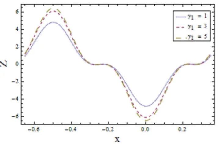
Figs. 9–16demonstrate the influence of embedded parameters on the heat transfer coefficient Z:The graphs signify the oscillatory behavior ofZ because of the propagation of peristaltic waves. Fig. 9 reveals that magnitude of heat transfer coefficient increases for compliant wall parametersE1,E2andE3. SinceE1,E2and E3 describes the elastic nature of wall that offer less resistance to heat transfer. Increasing values of Brinkman numberBr show similar behavior on heat transfer as of wall parameters. However the results obtained are much more distinguished in case of Br (seeFig. 10). The Biot numberc₁causes reduction in magnitude of heat transfer coefficient on the upper wall. Here thermal conductivity decreases with an increase in c₁ which lessens the impact of heat transfer coefficient near positive side (xw{₀:_{1) as depicted in Fig. 11. Reverse effect of Biot number c2} has been observed in the region fromFig. 12as heat transfer being directly related to Biot number dominates with an increase inc₂ which in turn increases the heat transfer distribution. Fig. 13shows decrease in heat transfer coefficient Z with Hall parameterm. Also in absence of Hall parameter(m~_{0)the results are much} more distinguished. The Hartman number m1 is an increasing function of heat transfer coefficient Z as fluid viscosity decreases with an increase in m1. The less viscous fluid particles will move through gain of higher kinetic energy that causes rise in transfer of heat (see Fig. 14). The effects of Weissenberg numberWe are displayed in Fig. 15. The obtained results show increase in transfer of heat when We increases as speed of wave increases with an increase inWe that supports the transfer of heat. The increasing values of power law index show decline in heat transfer distribution (see Fig. 16).

3.3 Homogeneous-Heterogeneous reactions effects

after a certain value ofgit starts decaying. This critical value ofgdepends on the strength of homogeneous reaction and it is prominent for increasing K. The effects of Schmidt number Sc are depicted in Fig. 19. The exhibited results are quite similar to Fig. 17. The drawn results follow by the fact that viscosity of fluid increases with an increase in Schmidt number that provides resistance to flow of fluid. The slow moving fluid particles have small molecular vibrations which lessen the concentration of fluid. As Schmidt number defines the ratio of viscous diffusion rate to molecular diffusion rate. Hence increasing values of Scenhances the viscous diffusion rate for fixed molecular diffusion rate which in turn helps to increase the concentration of fluid (see Fig. 19). The similar findings are reported by Shaw et al. [24].

3.4 Concluding remarks

The present analysis explores the effects of homogeneous and heterogeneous reactions in the peristalsis of Carreau fluid. Such analysis even for viscous fluid is yet not available. The major results of this study are listed below.

N

Similar behavior is observed for compliant wall parameters on temperature profile and heat transfer coefficient.

N

Temperature is increasing function of Brinkman number and Hall parameter.

N

The Biot numbers and Hartman number decrease the temperature of fluid.

N

Opposite effects of Weissenberg number We and power law index n are observed on the temperature profile and heat transfer coefficient.

N

Concentration of the reactants is more signified in case of homogeneous reaction parameter K than heterogeneous reaction parameter M.

Author Contributions

6. Ebaid A(2014) Remarks on the homotopy perturbation method for the peristaltic flow of Jeffrey fluid with nano-particles in an asymmetric channel. Comp Math Appl DOI: 10.1016/j.camwa.2014.05.008.

7. Abd-Alla AM, Abo-Dahab SM, Al-Simery RD(2013) Effect of rotation on peristaltic flow of a micropolar fluid through a porous medium with an external magnetic field. J Mag Mag Materials 348: 33–43.

8. Yasmin H, Hayat T, Alsaedi A, Alsulami HH(2014) Peristaltic flow of Johnson-Segalman fluid in an asymmetric channel with convective boundary conditions. Appl Math Mech 35: 697–716.

9. Mustafa M, Abbasbandy S, Hina S, Hayat T (2014) Numerical investigation on mixed convective peristaltic flow of fourth grade fluid with Dufour and Soret effects. J Taiwan Inst Chem Eng 45: 308–316.

10. Hayat T, Yasmin H, Alsaedi A(2014) Convective heat transfer analysis for peristaltic flow of power-law fluid in a channel. J Braz Soc Mech Sci Eng DOI: 10.1007/s40430-014-0177-4.

11. Parsa AB, Rashidi MM, Hayat T(2013) MHD boundary-layer flow over a stretching surface with internal heat generation or absorption. Heat Transfer–Asian Research 42: 500–514.

12. Abelman S, Momoniat E, Hayat T(2009) Steady MHD flow of a third grade fluid in a rotating frame and porous space. Nonlinear Analysis: Real World Appl 10: 3322–3328.

13. Rashidi MM, Ferdows M, Parsa AB, Abelman S (2014) MHD natural convection with convective surface boundary condition over a flat plate. Abstract and Applied Analysis 2014: 923487 (10 pages).

14. Merkin JH (1996) A model for isothermal homogeneous-heterogeneous reactions in boundary-layer flow. Math Comput Model 24: 125–136.

15. Zhang Y, Shu J, Zhang Y, Yang B(2013) Homogeneous and heterogeneous reactions of anthracene with selected atmospheric oxidants. J Environmental Sci 25: 1817–1823.

16. Kameswaran PK, Shaw S, Sibanda P, Murthy PVSN(2013) Homogeneous–heterogeneous reactions in a nanofluid flow due to a porous stretching sheet. Int J Heat Mass Transfer 57: 465–472.

17. Riaz A, Ellahi R, Nadeem S(2014) Peristaltic transport of a Carreau fluid in a compliant rectangular duct. Alexandria Eng J 53: 475–484.

18. Awais M, Farooq S, Yasmin H, Hayat T, Alsaedi A(2014) Convective heat transfer analysis for MHD peristaltic flow in an asymmetric channel. Int J Biomath 7: 1450023 (15 pages).

19. Ellahi R, Bhatti MM, Vafai K(2014) Effects of heat and mass transfer on peristaltic flow in a non-uniform rectangular duct. Int J Heat Mass Transfer 71: 706–719.

20. Tripathi D, Be´g OA(2014) A study on peristaltic flow of nanofluids: Application in drug delivery systems. Int J Heat Mass Transfer 70: 61–70.

21. Mustafa M, Hina S, Hayat T, Alsaedi A(2012) Influence of wall properties on the peristaltic flow of a nanofluid: Analytic and numerical solutions. Int J Heat Mass Transfer 55: 4871–4877.

22. Hina S, Hayat T, Alsaedi A(2013) Slip effects on MHD peristaltic motion with heat and mass transfer. Arab J Sci Eng 39: 593–603.