DOI: 10.1051/0004-6361:20041799 c
ESO 2005
Astrophysics
&
Investigation of flat spectrum radio sources by the interplanetary
scintillation method at 111 MHz
S. A. Tyul’bashev
1,2and P. Augusto
31 Pushchino Radio Astronomy Observatory, Pushchino, Moscow region 142290, Russia e-mail:serg@prao.psn.ru
2 Isaac Newton Institute, Chile, Pushchino Branch, Russia
3 Universidade da Madeira, Centro de Ciências Matemáticas, Caminho da Penteada, 9000-390 Funchal, Portugal
Received 5 August 2004/Accepted 18 April 2005
Abstract.Interplanetary scintillation observations of 48 of the 55 Augusto et al. (1998) flat spectrum radio sources were carried out at 111 MHz using the interplanetary scintillation method on the Large Phased Array (LPA) in Russia. Due to the large size of the LPA beam (1◦×0.5◦) a careful inspection of all possible confusion sources was made using extant large radio surveys:
37 of the 48 sources are not confused. We were able to estimate the scintillating flux densities of 13 sources, getting upper limits for the remaining 35. Gathering more or improving extant VLBI data on these sources might significantly improve our results. This proof-of-concept project tells us that compact (<1′′
) flat spectrum radio sources show strong enough scintillations at 111 MHz to establish/constrain their spectra (low-frequency end).
Key words.galaxies: general – galaxies: active – galaxies: quasars: general
1. Introduction
A systematic search for dominant structure on 0.09–0.3′′scales in large flat-spectrum radio source samples was made by Augusto et al. (1998). Fifty-five radio sources were selected from a parent sample containing 1665 strong flat-spectrum ra-dio sources (S8.4 GHz>100 mJy;α14..854 <0.5,Sν∝ν−α). These sources all have published MERLIN 5 GHz data. A few also have VLBA 5 GHz and MERLIN 22 GHz maps (Augusto et al. 1998). In addition, some others have MERLIN+EVN 1.6 GHz high angular resolution (<0.5′′) unpublished data (Augusto et al., in prep.).
The study of these 55 sources is not complete without low frequency observations (∼100 MHz), as was pointed out in Augusto et al. (1998), where the spectra of most sources have no data at all below∼300 MHz. The turnovers in the spectra of compact components in these sources must be found, to give a physical meaning to all 55 sources, namely by fitting syn-chrotron emission spectra for them all. Since VLBI does not routinely (or efficiently) operate at such low frequencies, we use the interplanetary scintillation (IPS) method at 111 MHz with the Large Phased Array (LPA). Very similar work was done at LPA for compact steep spectrum sources (Artyukh et al. 1999; Tyul’bashev & Chernikov 2000, 2001). The principle of IPS is very simple: the solar wind has variations in electron density on which depends the velocity of the radio waves that travel through it. As a result, we have a phase screen which can increase or decrease the signal from distant radio sources;
i.e. the sources willscintillate. The characteristic time of scin-tillations depends on the velocity of the solar wind, on the frequency of the observations, and on the sizes of the elec-tron clouds. For example, if we have observations at 111 MHz, this characteristic time scale is approximately one second. The scintillations will be stronger if the distant radio sources (or components therein) have small angular sizes (<1′′). Details of observations by the IPS method and relevant theory can be found, for example, in Vlasov et al. (1979).
The IPS method has advantages and disadvantages when compared with VLBI observations. The main advantage is the possibility to observe sources at low frequencies and high res-olution. The main disadvantage is the very low positional accu-racy. We see scintillations, but we do not know exactly which component(s) is(are) scintillating or even if we correctly iden-tify the main radio source (among many in-beam): the coordi-nate uncertainties for LPA are 5–10sin right ascension and 2–3′ in declination for strong sources (σscint/σnoise>2, atτ=0.5 s;
standardSNR>7), increasing to 30–60sand 5–7′, respectively, for weak sources (σscint/σnoise <2). These uncertainties have
a complex behaviour (f(σscint, σnoise); Artyukh & Tyul’bashev
1996). In order to get around these large, inherent errors (i.e. to, at least, correctly identify the source with the scintillating com-ponent) for all pointings that we have done with the LPA, we extensively searched the entire beam area using both the 1.4 GHz NRAO VLA Sky Survey (NVSS; Condon et al. 1998;www.cv.nrao.edu/nvss) and the 74 MHz VLA Low-Frequency Sky Survey (VLSS; lwa.nrl.navy.mil/VLSS).
The whole of Sect. 3 is devoted to this study. In Sect. 2, we present both the data collection and reduction, while in Sect. 4 we compile the IPS 111 MHz results from observations of 48 of the 55 Augusto et al. (1998) sources, for which we derive either a scintillating flux density estimate (13) or an upper limit (35). We also include in this section, as a case study, the detailed spectrum analysis for B0821+394. Finally, a short discussion and summary is given in Sect. 5.
2. Observations and data analysis
We carried out 111 MHz IPS observations with the LPA (a meridian instrument) of the Lebedev Institute of Physics, Russia. The effective area1 of the antenna in the zenith
di-rection is 2 × 10⁴ m2 with a beam approximately 1◦ ×0.5◦ (EW×NS) in size. The receiver integration time wasτ=0.5 s, the sampling time 0.1 s, and its bandwidth 600 kHz. As a re-sult, the sensitivity of LPA for scintillating sources isσscint ≃
0.15–0.2 Jy in the zenith direction (with SNR≥10, after the integration of all scintillations2), decreasing with source dec-lination as cos (δ), where δ is the declination of the source. The rms confusion due to extended (nonscintillating) sources is∼1 Jy, while the rms confusion due to scintillating sources is
≤0.12 Jy. This means that even when it is difficult to measure the total flux density of a source, it is still possible to measure the scintillating flux density.
We carried out 137 sessions in 2001–2002, each with a du-ration between 5 and 11 h. We observed, in each session, from 5 to 10 calibrators3and always less than 15 target sources. Thus,
a total of between 20 and 25 individual records were gath-ered per session and all targets were observed in more than one run (Non Col. (2) of Table B.3). The integration time for each source depended on its declination, so it varied from ap-proximately 9 to 18 min. In total, we had over 1100 h of obser-vation time, half of which on-target. Many individual source observations had to be prolonged to compensate for interfer-ence. Due to the large number of sources, it was not possible to choose the best elongation for each source as it was done in Artyukh (1981). Therefore, we used the converting coefficients of Marians (1975). We also selected the best data: the records, among the many observed, with the lowest noise.
Flat spectrum sources are very difficult to detect at low frequencies (in total flux density), therefore the data reduc-tion must be made with care (cf. similar steep-spectrum ra-dio source analysis in Tyul’bashev& Chernikov 2001). The data reduction method we used is given in Artyukh (1981) and Artyukh & Tyul’bashev (1996). This method enables us to detect faint scintillating sources, for which the scintillation dispersion (σ2scint) is smaller than the noise (dispersion) on the 1 Due to the large number of parameters on which the effective area depends, it can actually change by up to 20–30% from day to day.
2 Although we start up withσ
scint = σnoise ≃ 0.2 and τ = 0.5, the 9–18 min integration times assure 1080–2160 independent points. Since theSNRincreases with the square root of these, we getSNR≃ 30–45 which, being conservative, we translate intoSNR≥10.
3 We have amplitude calibrated the observations using many radio sources from the 3C/4C catalogues. All flux-density estimates were made in the scale of Kellermann (1964).
receiver time constantτ. We estimate this noise in the parts of the data record where we cannot see scintillations, i.e., where the noise seen is minimal. The accuracy of the scintillating flux density estimate (Scompact ≡ Sc) depends on the
fluctu-ation of the flux density (σscint) and on the elongation of the
source (angle between the Sun and source directions as seen by the observer). The typical accuracy is 20–25% for elongations smaller than 40◦andσ
scinthigher than the noise of the antenna
in a given direction. In the worst cases, the accuracy ofSc
es-timates is still better than 30–50% (see details in Artyukh & Tyul’bashev 1996; Artyukh et al. 1998).
Our observations lead to two situations: i) the compact source/components is/are too weak; no scintillations are de-tected but we can place an upper limit on the scintillation flux density (Sc); ii) scintillations are seen from a
com-pact component in the source. We try to get the best possi-ble estimate of Sc by combining all existing (good) records
(Col. (2) of Table B.3). The individual (statistical) error of a single record is 5–7%, hence combining them decreases it. Unfortunately, this error is overwhelmed by the calibration er-ror4at LPA (10–20%).
In what follows we summarize the observing/data reduction steps for each source (see also Sect. 4.2):
1. We observe one (or more) flux density calibrator(s) – sev-eral records.
2. We observe the target source (several records).
3. If possible, we estimate the total flux density (St) using the
calibrator and target records.Stadds the scintillating flux
density (compact component(s)) and the non-scintillating one (extended component(s)).
4. We look for scintillations in the target record by first remov-ing the background and then pulse interferences, havremov-ing only noise left (instrumental –σnoise – and scintillating – σscint). Then, we split these noises from the fact thatσnoise
exists all the time, whileσscintexists only from a given
di-rection –primaryrecord.
5. It is this latter part (few minutes) of the main record that is used to estimateScusingσscintand information on the
an-gular sizes of the source and its components (e.g. Marians 1975).
3. Confusion analysis
suit our purposes used the VLA-A at 8.4 GHz (0.2′′ resolu-tion): the Jodrell-VLA Astrometric Survey (JVAS; e.g. Patnaik et al. 1992) and the Cosmic Lens All-Sky Survey (CLASS; e.g. Myers et al. 2003). Apart from the main sources, which all have VLA-A 8.4 GHz compact components, only four “candidates”5
were detected by those surveys (see below).
There are three surveys of interest to our study. Although with much lower resolution than JVAS/CLASS, they were made at lower frequencies. The most relevant of these, at least as regards the frequency of observation, is the VLSS done with the VLA (B and BnA) at 74 MHz (80′′resolution). It certainly can identify the strongest sources in each of our LPA pointings but, unfortunately, it cannot tell us much about compactness. Another useful survey is the Faint Images of the Radio Sky at Twenty-centimeters (FIRST – Becker, White & Helfand 1995; sundog.stsci.edu/top.html), done with the VLA-B at 1.4 GHz (5′′resolution). Its resolution, although still three or-ders of magnitude above VLBI scales, is 16 times better than the one of VLSS, but the shift to high frequencies does not help much in our study. Unfortunately, both of the previous sur-veys lack full-sky coverage. The VLSS is still on-going, while FIRST covers less than half of the northern sky, where all our sources lie. As a result, out of the 48 pointings done with the LPA (centred on each of the main sources), 34 (71%) fell in-side the VLSS sky coverage while only 19 (40%) are in FIRST. The last survey we used in our study is the NVSS, made with the VLA (D and DnC) at 1.4 GHz (45′′resolution), which cov-ers the full northern hemisphere; hence, it should containall candidates to confusing sources of our observations.
Our “candidate-finding” scheme was to fully examine a 1.0◦×0.5◦area (equal to the LPA beam), centred on our main source position, using the Internet search engines in VLSS, NVSS, FIRST, and NED (the NASA Extragalactic Database; nedwww.ipac.caltech.edu), in order to get extra literature information (namely radio spectra and maps), if any. This has found a total of 1046 candidates for the 48 sources or “point-ings”6, the vast majority quite weak (Appendix A). All of
these are in the NVSS, but only 271 (out of the surveyed to-tal of 378 – 72%) and 29 (toto-tal 736, so 4%) aredetectedin FIRST (S1.4 >∼ 1 mJy/beam) and VLSS (S74 >∼0.5 Jy/beam),
respectively. A total of 135 candidates are in both surveyed areas, bringing the grand total of candidates with more in-formation than NVSS-only to 979, so only 67 (7%) lack it. Three candidates have only non-FIRST maps available while 36 others have only radio spectra as extra information: there are 82 candidates with spectral information of which 27 also have radio maps (see Table B.1). The question now is:how do we know if a candidate is strongly scintillating or not at 111 MHz? Obviously, the seven sources of Table B.1 with high resolution information (of which four also have FIRST maps) are the only
5 In the context of this section, acandidateis a source, inside each LPA pointing, that competes with our main source for the scintillations that we have observed (Table B.1 vs. Table B.3).
6 In this section we use the word “pointing” to refer to each beam area to be analysed: each 1.0◦×
0.5◦
area centred on each main source of the 48 observed and listed in Table B.3.
ones for which the best guess can be made. These are described, individually, in what follows:
J0117+321: in JVAS (e.g. Wilkinson et al. 1998), this source
shows up as compact (<0.2′′). However, it is a Giga-Hertz Peaked Spectrum (GPS) source and can be ruled out as can-didate since it is likely too weak at low frequencies.
J0823+391: also in FIRST (resolved; ∼30′′ wide large symmetric object with two edge-brightened lobes; 62 mJy/beam), this had further VLA observations done by Lehar et al. (2001) which show one of the lobes resolved (∼1′′ in size), the other compact (<0.7′′; 4 mJy/beam), as well as a central core (<0.7′′; <1 mJy/beam). It might contain VLBI compact components, but is possibly too weak to cause confusion; on this basis, we rule it out.
J0825+393: in FIRST, it is a bright (1106 mJy/beam)
unre-solved source; mapped with VLBI, it looks like a com-pact (size<0.07′′) steep spectrum source (Dallacasa et al. 2002). A definitely confusing candidate that must be kept.
J1013+493: a JVAS compact source (<0.1′′ – e.g. Patnaik
et al. 1992), it is actually a VLBI calibrator with a size< 0.02′′ (Beasley et al. 2002). In FIRST it shows up as a bright (266 mJy/beam) unresolved source. A definitely confusing candidate that must be kept.
J1215+331A: also known as NGC4203, this source has a
FIRST map available (slightly resolved; 6 mJy/beam). It very likely contains a central compact core (<1′′) with an inverted spectrum, possibly due to free-free absorption (e.g. Falcke et al. 2000; Ho & Ulvestad 2001). It shows an in-verted spectrum at high frequencies, most likely too weak at low frequencies to confuse our observations, so ruled out.
J2152+175: a core-plus-one-sided-jet VLBI source (e.g. Fey
& Charlot 1997), this source extends to very large struc-tures becoming a narrow angle tailed large radio galaxy (Rector & Stoke 2001). Both compact (<0.2′′) and ex-tended components are also seen in a VLA-A 8.4 GHz map (e.g. Browne et al. 1998). Its spectrum has a “knee” at ∼1 GHz, possibly peaking at <∼1 MHz: a typical core+halo spectrum. A definitely confusing candidate that must be kept.
J2154+174: slightly resolved (<0.01′′ size) with the VLBI
(Beasley et al. 2002) it is a VLA-A 8.4 GHz compact source (<0.1′′; Browne et al. 1998). Its spectrum has a “knee” at
∼1 GHz, possibly peaking at∼10 MHz (core+halo). A def-initely confusing candidate that must be kept.
As regards the remaining, to first order, the answer lies in the VLSS data. Only roughly half (15) of the 29 candidates are stronger than the respective main source, all lacking high res-olution maps for compactness determinations. The question is, then,how to proceed?In what follows, we will use all existing information we can in order toguessthe compactness of each. Taking advantage of existent spectral information, we de-cided to use the spectral index value between VLSS and NVSS (α1400
74 ) of each candidate, as compared to the
corre-sponding value of the main source (if existent), as indicative of the likelihood of a given candidate confusing the observations or not. Ifα1400
74 issteeperfor the candidate than for the main
and hence less probable of confusing our observations. Such comparison could be done for six of these 15 candidates, all re-jected as confusing candidates. What about the remaining nine? One of them (withα140074 = 1.0) has no further information, but we rule it out due to the comparison with the αfit ≃ 0.7
overall 232–1400 MHz spectrum of the corresponding main source which, in addition, has a GPS core-like component at 1.4–8.4 GHz. Four other candidates do have proper spectral information and the direct comparison using αfit rules them
all out; three have power-law spectra while the correspond-ing main source has a spectrum with a “knee”, suggestcorrespond-ing a halo+compact core source – so, in these cases, the candidates are not likely to confuse our observations (scintillations should come from the “core” component in the main source). The last one, however, peaks at ∼100 MHz, while the corresponding main source has a halo+core spectrum; hence, both sources might have compact components and we do not know which one is the stronger scintillator at 111 MHz. So, for caution, we keep it as confusion candidate.
What about the 14 candidates that are weaker than the main source? Although not confusing our observations, they might make some relevant contribution to the total scintillating flux density of the main source. Chasing their possible compactness properties, we useα140074 as above7to rule out all but four
can-didates that must be kept in the group because of their flatter values. As a matter of fact, two of these candidates have high resolution maps available (see Table B.1) confirming them with compact VLBI components.
The VLSS analysis is not yet complete, however: what about non-detections? Candidates in this situation must be ruled out only if the corresponding main source was indeed detected. Out of the 736 candidates surveyed by the VLSS, 683 (93%) are thus ruled out in three different situations: i) 277 (NVSS) candidates reside in the 19 VLSS “pointings” that found no confusing candidates at all; ii) 356 candidates in the remaining 14 VLSS “pointings” with a detected main source stronger than each of them; iii) 50 “control” candi-dates, with FIRST and/or spectra information (six have both; see Table B.1).
With the hope of making use of the extant FIRST/NVSS data for the 309 candidates left that were not surveyed by VLSS8, we tried to define and calibrate criteria for ruling out
candidates. For this, we used both the 50 “control” candi-dates not detected in the VLSS and the 21extracandidates in Table B.1 that actually have both FIRST and radio spectra in-formation (Appendix B) – six of the 27 candidates in Table B.1 are included in the 50 “control” candidates (N.D. in Col. (7) of Table B.1). This, however, was not possible, since both a combined classification and a separate one failed the calibra-tion tests. Hence, since there is no strong statistical basis to rule out (or not) a candidate using FIRST and/or spectral informa-tion, being conservative, we keep all 333 remaining candidates, regardless of their extra information. In a final attempt to split this number into highest/lowest probabilities of confusing our
7 And, in one case, also spectral information.
8 One of such candidates (J0823+391) was actually ruled out before thanks to a VLA map – see text above.
observations, we used 1.4 GHz NVSS flux density information (cf. Appendix A) to reason as follows: if a source is too weak, its spectrum would have to be too steep to reach “confusion levels”, i.e., to have a comparable low frequency flux density to the respective main source. This time, we must set an arbi-trary limiting value:α = 1.5. Steeper candidates are rejected. Using, then, the lowest frequency (lo) with measured flux density for each respective main source (on 151–356 MHz), 262 candidates do not reach 20% of that value keepingαNVSS
lo <
1.5 and are, thus, rejected. The 71 candidates left can be fur-ther split into 16 included in Table B.2, with the highest proba-bility of causing confusion (they reach main source flux den-sities within αNVSS
lo < 1.5), and 53 other (in the fields of
14 main sources with “confused?” or “confused” in Col. (10) of Table B.3) which reach 20–100% of each low frequency main source flux densities withinαNVSSlo <1.5.
In Table B.2 we present the final list of 23 high probabil-ity confusing candidates, corresponding to the 11 main sources signaled with “confused” in Col. (10) of Table B.3. Thus only about 23% of our observed sources might have a good probabil-ity of being confused. It is impossible to make any better state-ment based on extant data since, to some degree, all 48 sources might be confused. Only detailed VLBI observations of all 1046 candidates might establish definitive conclusions.
4. Results
4.1. Overall
The results of our observations are presented in Table B.3. We observed 50 sources from the sample of 55 sources in Augusto et al. (1998) but only got scintillating flux den-sity data for 48 (87% completeness): five sources have not been observed because of their high declinations (δ > 70◦), resulting in too poor elongations9 – B0205+722,
B0352+825, B0817+710, B0916+718, B1241+735; two other (B0905+420 and B1003+174) were confused by nearby strong VLBI sources (B0904+417 and B1004+178, respectively), so no information aboutScis available for these either.
The IPS method requires knowledge of the upper limit for the (at least; ideally the actual) size of the scintillating compo-nent of a radio source in order to measure its flux density accu-rately. We should gather as much size information as possible for all compact components of each (e.g. Artyukh et al. 1999). This was not possible for the 17 sources in Table B.3 (35% of the total), indicated with a star (⋆) after their names, for which either VLBI data are not available or there is still ambiguity in identifying the scintillating component: theirSc should have
their current uncertainties much reduced if/when those data are collected. For example, the source B1058+245 has three components (Augusto et al. 1998). The two at northeast have
9 Ideally, these should be on 22◦
–40◦
angular sizes 0.062×0.022′′(A) and 0.103×0.053′′(B), and are separated by 0.047′′. The southwest component has size 0.314 × 0.094′′ (C), and is 0.8′′ away from the other two. Scintillations from all components will add simultaneously, combining their flux densities. Hence, we do not know which component(s) contributes most at 111 MHz, because we do not have spectral information for each component. If it is compo-nent A, we get Sc <0.27 Jy; if component C we get Sc <
0.5 Jy. Thus, we put the value<0.5 Jy (hoping to improve it in the future) in Col. (7) of Table B.3.
When possible, we have thoroughly investigated the struc-ture of each source from the published (high frequency) VLBI-maps (Cols. (4) and (5) in Table B.3). We checked (when possible) whether the spectra of compact components are peaked at high frequencies. These components should not dominate at low frequencies and we excluded them from fur-ther consideration. We also excluded components which have less than five times the flux density of any other component. Among the remaining compact components, we tried to find those with a comparatively high flux density and steep spec-trum at high frequencies and assumed that they have power-law spectra down to low-frequency. Such an analysis allows us to reveal one or several components of known angular size domi-nating at 111 MHz.
In Col. (8) of Table B.3 we show the total flux densi-ties at 74 MHz from the VLSS while in Col. (9) we present the α140074 spectral index with the help of the NVSS. Out of the 48 sources, 33 (69%) have, at least, some indication of flux density at 74 MHz (seven are below 5σ), while only one (B0529+013) is not detected. The remaining 14 sources are not in the current VLSS sky coverage.
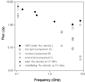
4.2. Case study: B0821+394
We have chosen B0821+394 as a case study because it demon-strates all features typical of scintillating sources. It has the strongest scintillation in our sample (Col. (7), Table B.3), al-lowing us to even estimateσscint“by eye” from Fig. 1. It has
enough total flux density to subtract the background. Finally, it has a lot of observations at high angular resolution, and there-fore we can do an accurate analysis of its structure in order to guess which compact components will dominate at 111 MHz.
Our observations of B0821+394 were obtained during six days at elongations from 34◦to 46◦accumulating to a to-tal of 105 min. The value ofσscint varied substantially from
session to session of observations, therefore we have a large error (25%) in our estimation ofSc– Table B.3. With an even
larger error we could measure its total flux density (St).
The radio source B0821+394 is a complicated SE-NW core-plus-one-sided-jet with redshift 1.216 (Wills & Wills 1976; Augusto et al. 1998). This source has previously been observed with high angular resolution (1.6 GHz – MERLIN, 8.4 GHz – VLA-A, 5 GHz – VSOP; references in Col. (5) of Table B.3) and from these data we can model it, to first order, with three main components: A) NW “hot spot” with angular size 11 × 9 milliarcseconds (mas) at PA = −38◦ and ∼250 mas away from the nucleus; B) SE nucleus with
Fig. 1.Primary record of the strong scintillating source B0821+394. The comparison between “scintillation+noise” and “noise” gives us the possibility of estimating pure scintillations. The details of reduc-tion of such observareduc-tions are, for example, in Artyukh & Tyul’bashev (1996).
Fig. 2.Spectrum of the source B0821+394 and spectra of its compact components (NED – NASA Extragalactic Database).
size <0.3×< 0.5 mas; C) SE “knot” (start of jet) with size 2×<0.7 mas at PA=−18◦, and∼13 mas away from the nu-cleus. Since components A, B, and C are so close and compact, B0821+394 will scintillate strongly from all, simultaneously. Hence, the flux densities of these compact components add to give the result in Col. (7) of Table B.3. However, as we see next, only one of these components can dominate at 111 MHz. Building the spectra of components A, B, and C from informa-tion in the literature (Fig. 2), we see that the nucleus (B) has a GHz-peaked spectrum (decreasing to low frequencies), while components A and C have power-law spectra. We have an over-all flat spectrum source, as was previously known (Augusto et al. 1998). Our estimation of the total flux density (6.5±2 Jy) agrees with other data while the scintillating flux density from components A and C is 2.5±0.6 Jy.
5. Discussion
are, generally, much weaker (in St) than the steep-spectrum
radio sources investigated earlier (Tyul’bashev& Chernikov 2001). We found that one-fourth (13 out of 48) of the flat-spectrum sources observed by us got estimates inSc that,in the worst scenario, have errors smaller than 35% (Table B.3), with one exception at<50%. We were even able to determine Stwithin 60% errors for the five strongest sources. How in the
future can we improve our estimations ofSc? Simply by
get-ting proper multi-frequency high resolution observations that might enable us to identify the scintillating component(s) at 111 MHz. This next step is well under way (Augusto et al., in preparation). As regards the 35 sources with upper limits (only), we might improve them substantially or, better, trans-form them into actualSc estimates, with the advent of high
resolution data.
The previous results, however, had to be strengthened, due to the large LPA beam (1◦ × 0.5◦), by making sure that most targets were not affected by confusion. Due to the lack of more appropriate surveys, 1046 confusion candi-dates were identified by an extensive search in NVSS (sur-veying 100% of candidates), VLSS (70%), FIRST (36%), and NED. Of these, only seven (0.7%) have published high resolution maps (VLBI/VLA). It is tantalizing that 97% of the candidates residing in the VLSS 74 MHz surveyed areas (683 candidates, or 93% of the total number) were not detected (S74 < 0.5 Jy/beam), while the respective targets were so, all
but one; and out of the remaining 3% (29 candidates), using the steepness of α1400
74 (and VLBI maps for two) when compared
with the corresponding main source, only five (17%) were not ruled out as causing confusion. Four other candidates were maintained thanks to detailed VLBI maps. Using detailed spec-tral information (for two) and VLA maps, three further candi-dates were ruled out. Finally, 262 extra candicandi-dates that cannot reach 20% of the main source low frequency (lo) flux density withinαNVSS
lo <1.5 were ruled out; 53 that reach 20–100% are
low probability confusion candidates while the remaining 16 join seven others from the map/spectra selection (Table B.2) as the highest probability candidates for causing confusion: only 11 (23%) of the 48 main sources are thus affected.
As was pointed out in Augusto et al. (1998), 31 out of their 55 sources (56%) have no data below∼300 MHz. The observa-tions presented in this paper might be a breakthrough for estab-lishing the low-frequency spectra of the 55 sources in Augusto et al. (1998), since 48 were observed, meaning 87% complete-ness. Relevant new information from our data comes from the estimates on Scat 111 MHz as compared with the total flux
densities at 74/151 MHz from the literature (e.g. Augusto et al. 1998 and Table B.3) – we can place an approximate upper limit on the flux densities of extended low surface brightness com-ponents, for the sources10 B0116+319 (<
∼0.4 Jy), B0824+355
(<∼1.5 Jy), and B1211+334 (<∼1.5 Jy).
Knowledge of the low-frequency end of the radio spectrum of a radio source (and its components) is vital before fitting any synchrotron emission model to gain knowledge about its
10 Using the minimum possible value as a lower limit for the flux density in compact components; e.g. 0.7±0.2 Jy gives us a lower limit of 0.5 Jy.
physical properties. Our objective, in due course, is to make such fits for all 55 sources. There is potential for all but one source since, in addition to the 48 presented in this paper, six out of the seven left out actually have 151 MHz total flux densities in the literature. Since these exist in two main types (core+(distorted)-jets; compact/medium symmetric objects – believed to be the precursors of large FRI/FRII radio galaxies), we think we can contribute to clarifying the origin of this sub-set of active galactic nuclei, at least as regards their emission mechanisms.
Acknowledgements. We acknowledge an anonymous referee for helpful suggestions and comments. We are grateful to R. D. Dagkesamanskii for attention to our work and for hosting P. Augusto during his visit. S. A. Tyul’bashev acknowledges the programs “Solar Wind” and “Extended sources” from the Russian Academy of Sciences for the partial support of this work. P. Augusto acknowl-edges the research grant PESO/P/PRO/15133/1999 from the Fundação para a Ciência e a Tecnologia (Portugal). This research made use of the United States Naval Observatory (USNO) Radio Reference Frame Image Database (RRFID) and of the NASA Extragalactic Database (NED).
Appendix A: the flux densities of the confusion candidates
As regards NVSS flux densities, out of the 1046 candidates, 950 (91%) have 1.4 GHz flux densities<37 mJy. This leaves 96 strong (≥37 mJy) candidates11, of which 28 are also in the
VLSS. It is tantalizing that, out of these 96 “strong” candidates, only four, in three pointings, have NVSS 1.4 GHz flux densities stronger than the corresponding main source with flux density ratios 1.6, 1.1, 2.9 and 1.3, respectively.
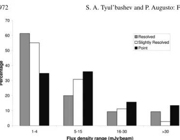
For all three FIRST types [i) unresolved (U); ii) slightly resolved (S R); iii) resolved (R)] – see Appendix B, the weakest detected source has 1 mJy/beam. In Fig. B.1 we present the flux density distributions for each type. Comparing the flux density distributions up toS1.4 = 15 mJy/beam, we exclude 29% of
unresolved sources, 14% of slightly resolved ones, and 19% of resolved sources. Going further down toS1.4 ≤4 mJy/beam,
the respective exclusion rates are 65%, 45%, and 39%, thus showing a trend for the weakest sources to be resolved.
The comparison of the VLSS flux densities between the candidates and each corresponding main source is only possi-ble for 13 pointings (out of 19), corresponding to 20 candidates (out of 29), since for the remaining there are no VLSS flux den-sity measurements of the main source. Overall, the flux denden-sity ratios are in the range 0.2–4.1 with all but two candidates in the interval 0.4–2.6. Hence, the typical candidate-main source flux density ratio is within a factor of about 2.5.
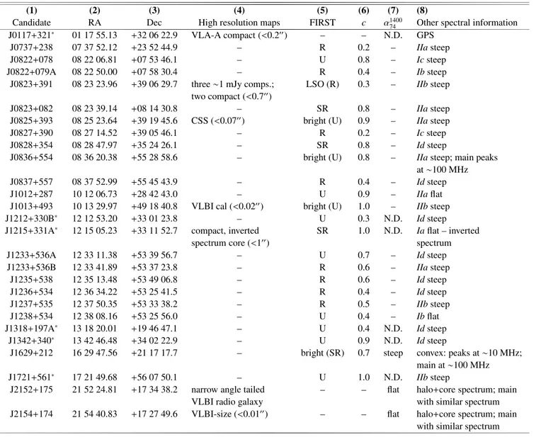
Table B.1.The 27 confusion candidates that have both radio structure and radio spectra information.(1): The J2000.0 name of the candidate; marked with an asterisk are “control” candidates (see main text);(2): 2000.0 right ascension from the NVSS;(3): 2000.0 declination from the NVSS;(4): short description of the source morphology with high resolution maps (VLBI and VLA), including sizes; CSS: compact steep spectrum source;(5): morphological description from FIRST, if surveyed (LSO: large symmetric object; U: unresolved; SR: slightly resolved; R: resolved); “bright” meansSFIRST
1.4 >170 mJy – all other sources haveS FIRST
1.4 <110 mJy;(6): the compactness parameter (S FIRST 1.4 /S
NVSS 1.4 ); (7): the spectral index as compared with the main source value calculated from the VLSS (if surveyed; N.D. means no detection in VLSS) and the NVSS;(8): compared spectral indices from other frequencies (subgroups as in Appendix B); when detailed spectral information exists, it is described; GPS – Gigahertz Peaked Spectrum Source.
(1) (2) (3) (4) (5) (6) (7) (8)
Candidate RA Dec High resolution maps FIRST c α1400
74 Other spectral information J0117+321∗
01 17 55.13 +32 06 22.9 VLA-A compact (<0.2′′
) – – N.D. GPS
J0737+238 07 37 52.12 +23 52 44.9 – R 0.2 – IIasteep
J0822+078 08 22 06.81 +07 53 46.1 – U 0.8 – Icsteep
J0822+079A 08 22 50.00 +07 58 30.4 – R 0.4 – Ibsteep
J0823+391 08 23 23.96 +39 06 29.7 three∼1 mJy comps.; LSO (R) 0.3 – IIbsteep two compact (<0.7′′)
J0823+082 08 23 39.14 +08 14 30.8 – SR 0.8 – IIasteep
J0825+393 08 25 23.64 +39 19 45.6 CSS (<0.07′′
) bright (U) 0.9 – IIasteep
J0827+390 08 27 14.52 +39 05 46.1 – R 0.2 – Icsteep
J0828+354 08 28 47.97 +35 24 26.1 – SR 0.8 – Idsteep
J0836+554 08 36 20.38 +55 28 58.6 – bright (U) 0.8 – IIasteep; main peaks
at∼100 MHz
J0837+557 08 37 52.99 +55 45 43.9 – R 0.4 – Idsteep
J1012+287 10 12 06.73 +28 42 43.0 – U 0.9 – IIaflat
J1013+493 10 13 29.97 +49 18 40.8 VLBI cal (<0.02′′
) bright (U) 1.0 – IIbsteep
J1212+330B∗
12 12 53.20 +33 01 23.8 – U 0.3 N.D. Idsteep
J1215+331A∗
12 15 05.23 +33 11 52.7 compact, inverted SR 1.0 N.D. Iaflat – inverted
spectrum core (<1′′) spectrum
J1233+536A 12 33 11.38 +53 39 56.7 – U 0.7 – Idsteep
J1233+536B 12 33 41.89 +53 37 23.8 – R 0.6 – IIasteep
J1235+538 12 35 13.48 +53 49 06.8 – R 0.6 – Idsteep
J1236+534 12 36 34.22 +53 25 41.5 – R 0.4 – Idsteep
J1237+535 12 37 50.35 +53 33 38.2 – R 0.5 – IIbsteep
J1238+534 12 38 08.16 +53 25 56.0 – U 0.4 – Ibflat
J1318+197A∗
13 18 20.01 +19 46 47.1 – U 0.4 N.D. Idsteep
J1342+340∗ 13 42 46.48 +34 02 22.9 – U 0.9 N.D. Idsteep
J1629+212 16 29 47.56 +21 17 17.7 – bright (SR) 0.7 steep convex: peaks at∼10 MHz; main at∼100 MHz
J1721+561∗ 17 21 49.68 +56 07 50.1 – U 1.0 N.D. IIbsteep
J2152+175 21 52 24.81 +17 34 38.2 narrow angle tailed – – flat halo+core spectrum; main
VLBI radio galaxy with similar spectrum
J2154+174 21 54 40.83 +17 27 49.6 VLBI-size (<0.01′′
) – – flat halo+core spectrum; main
with similar spectrum
Appendix B: FIRST/spectral classification
As regards to the use of spectral information, in the hope of applying a similar spectral criterion to the one applied for the 29 VLSS candidates (Sect. 3), as before, depending on the number and range of the data points, we split the 60 candidates with spectral information into two large groups (usually the main source has more data points than each cor-responding candidate and includes data at all available fre-quencies):two data points – group I– two-frequency spectral index calculation, compared with the same spectral index for the main source;three to five data points – group II– a lin-ear regression is made (a global spectral index is fitted) and the result is compared with the one obtained by applying the
same technique to the corresponding main source, using the same frequency range. Then, depending at which frequencies they have data, we split them further into the following seven subgroups (between brackets the number of candidates inside each subgroup):Ia)1.4–2.7 GHz (1); Ib)1.4–4.85 GHz (8); Ic)(318 or 365 or 408) to 1400 MHz (27);Id)151–1400 MHz (8); IIa) 3-point fit; 151–408 MHz to 1.4–4.85 GHz (12); IIb)4-point fit; 74–365 MHz to 4.85–8.4 GHz (3);IIc)5-point fit; 151 MHz to 4.85 GHz (1). The 60 candidates were then classified as “steep” or “flat” relative to the respective main source (cf. Table B.1). “Steep” cases would be expected to be ruled out as candidates, while “flat” ones would be kept in.
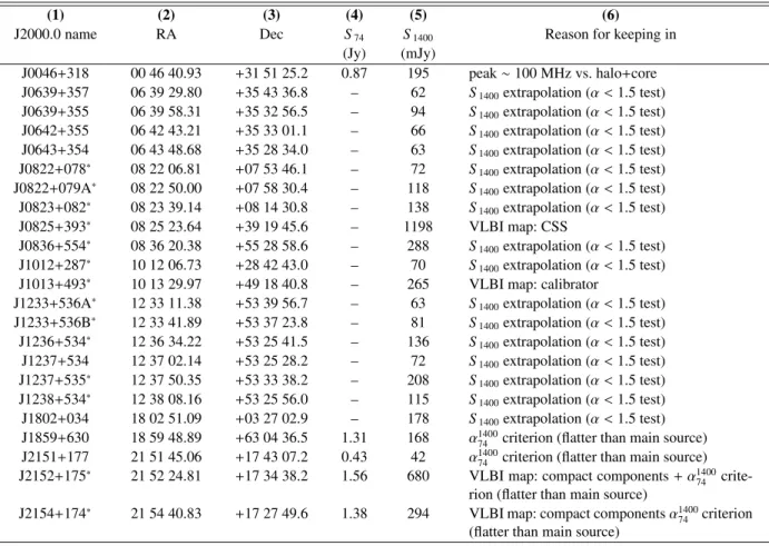
Table B.2.The 23 sources that most likely confuse our observations.(1): The J2000.0 name of the candidate; the sources marked with an asterisk are also listed in Table B.1;(2): 2000.0 right ascension from the NVSS;(3): 2000.0 declination from the NVSS;(4): the VLSS 74 MHz flux density;(5): the NVSS 1.4 GHz flux density;(6): short description of the reason for keeping the candidate as a confusing source; CSS: compact steep spectrum source.
(1) (2) (3) (4) (5) (6)
J2000.0 name RA Dec S74 S1400 Reason for keeping in
(Jy) (mJy)
J0046+318 00 46 40.93 +31 51 25.2 0.87 195 peak∼100 MHz vs. halo+core J0639+357 06 39 29.80 +35 43 36.8 – 62 S1400extrapolation (α <1.5 test) J0639+355 06 39 58.31 +35 32 56.5 – 94 S1400extrapolation (α <1.5 test) J0642+355 06 42 43.21 +35 33 01.1 – 66 S1400extrapolation (α <1.5 test) J0643+354 06 43 48.68 +35 28 34.0 – 63 S1400extrapolation (α <1.5 test) J0822+078∗
08 22 06.81 +07 53 46.1 – 72 S1400extrapolation (α <1.5 test) J0822+079A∗
08 22 50.00 +07 58 30.4 – 118 S1400extrapolation (α <1.5 test) J0823+082∗ 08 23 39.14 +08 14 30.8 – 138 S
1400extrapolation (α <1.5 test) J0825+393∗
08 25 23.64 +39 19 45.6 – 1198 VLBI map: CSS J0836+554∗
08 36 20.38 +55 28 58.6 – 288 S1400extrapolation (α <1.5 test) J1012+287∗
10 12 06.73 +28 42 43.0 – 70 S1400extrapolation (α <1.5 test) J1013+493∗ 10 13 29.97 +49 18 40.8 – 265 VLBI map: calibrator
J1233+536A∗ 12 33 11.38 +53 39 56.7 – 63
S1400extrapolation (α <1.5 test) J1233+536B∗
12 33 41.89 +53 37 23.8 – 81 S1400extrapolation (α <1.5 test) J1236+534∗
12 36 34.22 +53 25 41.5 – 136 S1400extrapolation (α <1.5 test) J1237+534 12 37 02.14 +53 25 28.2 – 72 S1400extrapolation (α <1.5 test) J1237+535∗
12 37 50.35 +53 33 38.2 – 208 S1400extrapolation (α <1.5 test) J1238+534∗
12 38 08.16 +53 25 56.0 – 115 S1400extrapolation (α <1.5 test) J1802+034 18 02 51.09 +03 27 02.9 – 178 S1400extrapolation (α <1.5 test) J1859+630 18 59 48.89 +63 04 36.5 1.31 168 α1400
74 criterion (flatter than main source) J2151+177 21 51 45.06 +17 43 07.2 0.43 42 α1400
74 criterion (flatter than main source) J2152+175∗
21 52 24.81 +17 34 38.2 1.56 680 VLBI map: compact components+α1400 74 crite-rion (flatter than main source)
J2154+174∗
21 54 40.83 +17 27 49.6 1.38 294 VLBI map: compact componentsα1400 74 criterion (flatter than main source)
plots), and decided to split the morphologies of the 271 candidates found into three groups: i) unresolved sources (<5′′ in size;U) – 89 candidates (33%); ii) slightly resolved sources (∼5′′in size;S R) – 107 candidates (39%); iii) resolved sources (>5′′in size;R) – 75 candidates (28%) (Fig. B.1).
Noting that FIRST alone gives a very poor indication on the existence or not of VLBI compact structure, we decided to include also information from NVSS, using the ratio of both 1.4 GHz flux densities (SFIRST/SNVSS) to define acompactness
(c) parameter. Since the NVSS beam is nine times the width of the FIRST beam (81 times in area) it is also a lot more sensitive to extended structure. Thus, we would expect a point source to havec=1 while a very resolved source would have c ≪ 1. Indeed, although with large dispersions, the averages arec=0.8 (U),c=0.7 (S R), andc=0.4 (R). We have, then, decided to use these criteria together in order to defineresolved candidates (to be ruled out as confusing candidates) as the ones with12 (R∨S R)∧c ≤0.6 andunresolved(to be kept in) the
ones with (U∨S R)∧c≥0.9. Any other situations would not be considered, since they were too ambiguous. It must be em-phasized that even aU∧c= 1.0 candidate is not guaranteed to have compact VLBI structure, since the FIRST resolution 12 For the rest of this Appendix we used the logical symbols ∨ (for OR) and∧(for AND) in order to compactify the exposition.
is 5′′. Variability complicates the picture: some sources have been observed some years apart between the two surveys. For example, values ofc>1 (27 candidates in 271; 10%) must be due to variability. We expect FIRST unresolved sources (likely containing cores) to be more variable than extended ones; in-deed, 15 of the 27 variable candidates (56%) are “unresolved” while “slightly resolved” are the remaining (44%) – there are no variable “resolved” candidates.
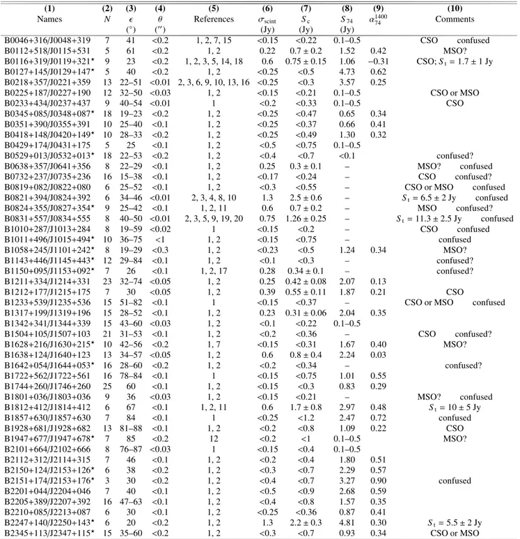
Table B.3.The scintillating flux density (or upper limit) of the scintillating component(s) at 111 MHz for 48 of the 55 sources in Augusto et al. (1998).(1): B1950.0 and J2000.0 names; when a star (⋆) follows, it means that the source has the potential to get improved values of flux densities limited/measured, when relevant VLBI data are available.(2): The amount of individual records.(3): The elongation range during the observations.(4): The maximum size of the scintillating component, estimated from the high-resolution information on the references listed in (5)and (still) unpublished VLBI maps (Augusto et al., in prep.).(5): References for the high resolution maps used, with code numbers translated at the footnote of this table.(6): 111 MHz dispersion (σscint) during a scintillation across thefullobservation range (cf. Fig. 1).(7): 111 MHz scintillation flux density (Sc) measurements with error, or upper limit.(8): Total flux density at 74 MHz (from the VLSS); sources with a range given are detected but not above 5σ.(9): Spectral index between 74 MHz (VLSS) and 1.4 GHz (NVSS).(10): General comments/information where we give: i) the total 111 MHz flux densities (St) for the five sources for which this was possible to measure (SNR>30); ii) CSO-MSO (compact-medium symmetric object) classification, after Augusto et al. (1998) and Augusto et al. (1999); iii) other information.
(1) (2) (3) (4) (5) (6) (7) (8) (9) (10) Names N ǫ θ References σscint Sc S74 α140074 Comments
(◦
) (′′
) (Jy) (Jy) (Jy)
B0046+316/J0048+319 7 41 <0.2 1, 2, 7, 15 <0.15 <0.22 0.1–0.5 CSO confused B0112+518/J0115+531 5 61 <0.2 1, 2 0.22 0.7±0.2 1.52 0.42 MSO? B0116+319/J0119+321⋆ 9 23 <0.2 1, 2, 3, 5, 14, 18 0.6 0.75±0.15 1.06 −0.31 CSO;S
t=1.7±1 Jy B0127+145/J0129+147⋆ 5 40 <0.2 1, 2 <0.25 <0.5 4.73 0.62
B0218+357/J0221+359 13 22–51 <0.01 2, 3, 6, 9, 10, 13, 16 <0.25 <0.3 3.57 0.25
B0225+187/J0227+190 12 32–50 <0.03 1, 2 <0.15 <0.21 0.1–0.5 CSO or MSO B0233+434/J0237+437 9 40–54 <0.01 1 <0.2 <0.33 0.1–0.5 CSO B0345+085/J0348+087⋆ 18 19–23 <0.2 1, 2 <0.25 <0.47 0.65 0.34
B0351+390/J0355+391 10 25–40 <0.1 1, 2 <0.25 <0.37 0.66 0.41 B0418+148/J0420+149⋆ 10 28–33 <0.2 1, 2 <0.25 <0.49 1.30 0.32 B0429+174/J0431+175 5 25 <0.1 1, 2 <0.5 <0.75 0.1–0.5
B0529+013/J0532+013⋆ 18 22–53 <0.2 1, 2 <0.4 <0.7 <0.1 confused? B0638+357/J0641+356 8 22–29 <0.1 1, 2 0.25 0.3±0.1 – MSO? confused B0732+237/J0735+236 16 15–38 <0.1 1, 2 <0.17 <0.24 – CSO confused? B0819+082/J0822+080 6 25–52 <0.1 1, 2 <0.3 <0.55 – CSO or MSO confused B0821+394/J0824+392 6 34–46 <0.01 2, 3, 4, 8, 10 1.3 2.5±0.6 – St=6.5±2 Jy confused B0824+355/J0827+354⋆ 9 25–42 <0.1 1, 2, 11 0.6 0.7±0.2 – MSO confused? B0831+557/J0834+555 8 40–50 <0.01 2, 3, 5, 9, 19, 20 0.75 1.26±0.25 – St=11.3±2.5 Jy confused B1010+287/J1013+284 8 19–59 <0.02 1 <0.15 <0.2 – CSO confused B1011+496/J1015+494⋆ 10 36–75 <1 1, 2 <0.15 <0.75 – confused B1058+245/J1101+242⋆ 8 19–29 <0.3 1, 2 <0.23 <0.5 1.24 0.34 MSO? B1143+446/J1145+443⋆ 12 29–84 <0.1 1, 2 <0.1 <0.3 – confused? B1150+095/J1153+092⋆ 7 26 <0.1 1, 2, 17 0.28 0.34±0.1 – confused? B1211+334/J1214+331 23 32–74 <0.05 1, 2 0.25 0.42±0.08 2.07 0.13
B1212+177/J1215+175 7 30 <0.05 1, 2 0.39 0.55±0.11 1.87 0.21 CSO
B1233+539/J1235+536 15 51–82 <0.1 1 <0.15 <0.37 – CSO or MSO confused B1317+199/J1319+196 15 28–52 <0.1 1, 2 0.23 0.31±0.06 2.04 0.35
B1342+341/J1344+339 15 43–60 <0.03 1, 2 <0.1 <0.22 0.1–0.5
B1504+105/J1507+103 21 31–53 <0.1 1, 2 <0.2 <0.36 – CSO confused? B1628+216/J1630+215⋆ 10 42–56 <0.2 1, 7 <0.15 <0.31 1.67 0.40 MSO? B1638+124/J1640+123 13 34–57 <0.05 1, 2 0.6 0.8±0.4 2.24 0.03
B1642+054/J1644+053⋆ 16 28–60 <0.2 1, 2 <0.2 <0.34 – confused? B1722+562/J1722+561 16 78–84 <0.1 1 <0.15 <0.75 1.01 0.55
B1744+260/J1746+260 25 60 <0.1 1, 2 <0.15 <0.3 0.83 0.29
B1801+036/J1803+036 9 36 <0.03 1, 2 <0.15 <0.21 – MSO? confused B1812+412/J1814+412 6 67 <0.1 1, 2, 11 0.6 1.7±0.8 2.97 0.48 St=10±5 Jy B1857+630/J1857+630 7 84 <0.1 1 <0.25 <1.2 2.47 0.72 confused B1928+681/J1928+682 13 81–88 <0.1 1, 2 <0.2 <0.8 1.09 0.22 CSO B1947+677/J1947+678⋆ 7 85 <0.2 12 <0.2 <1 0.1–0.5 MSO? B2101+664/J2102+666 8 76–87 <0.03 1 <0.15 <0.4 0.1–0.5
B2112+312/J2114+315 7 46 <0.1 1, 2 <0.2 <0.4 1.80 0.51 B2150+124/J2153+126⋆ 6 38 <0.2 1, 2 <0.3 <0.7 2.29 0.57
B2151+174/J2153+176⋆ 3 30 <0.2 1, 2 <0.4 <0.7 3.27 0.90 confused B2201+044/J2204+046 7 40 <0.1 1, 2 <0.5 <0.9 2.68 0.59
B2205+389/J2207+392 16 47–63 <0.1 1, 2 <0.4 <0.8 1.57 0.35 B2210+085/J2213+087 6 30 <0.1 1, 2 <0.25 <0.36 0.87 0.41
B2247+140/J2250+143⋆ 6 20 <0.2 1, 2 1.3 2.2±0.3 4.81 0.30 S
t=5.5±2 Jy B2345+113/J2347+115⋆ 15 35–60 <0.2 1, 2 <0.3 <0.7 0.93 0.34 CSO or MSO
Fig. B.1.The FIRST flux density distributions of the 271 candidates with such data, divided into the classifications “resolved”, “slightly resolved”, and “point”. The averages are, respectively, 11 mJy/beam, 9 mJy/beam, and 20 mJy/beam.
nine are immediately ignored as FIRST ambiguous, only other nine of the remaining 11 have consistent FIRST/spectral infor-mation ((S R∨R)∧c ≤ 0.6 and steep; (S R∨U)∧c ≥ 0.9 and flat). Taking our “calibration” further, we also looked, sep-arately as it could only be, at FIRST and spectral decisions for the remaining 44 “control” candidates: i) 13 candidates with FIRST data split into two variable, four ambiguous, two with (S R∨U)∧c ≥ 0.9 and five with (S R∨R)∧c ≤ 0.6; ii) 31 candidates with spectral data split into 19 steep, three flat (Ic); two steep, one flat (II); and six flat (Ib), of which four have inverted spectra. To add even more information on this, we have used 95 candidates with FIRST (S R∨R)∧c≤0.6 and (S R∨U)∧c≥0.9 classifications (which are not mentioned anywhere else in this paper) which split into two suspiciously size-comparable samples, with 50 in the former classification and 45 in the latter. Hence, our FIRST and/or spectra criteria fail too often to be of any use for decisions on candidates which only have these data available, in addition to NVSS.
References
Altschuler, D. R., Gurvits, L. I., Alef, W., et al. 1995, A&AS, 114, 197 Artyukh, V. S. 1981, SvA, 25, 116 (AZh 58, 208)
Artyukh, V. S., & Tyul’bashev, S. A. 1996, Astron. Rep., 40, 608 (AZh 73, 669)
Artyukh, V. S., Tyul’bashev, S. A., & Isaev, E. A. 1998, Astron. Rep., 42, 283 (AZh 75, 323)
Artyukh, V. S., Tyul’bashev, S. A., & Chernikov, P. A. 1999, Astron. Rep., 43, 1 (AZh 76, 3)
Augusto, P., Wilkinson, P. N., & Browne, I. W. A. 1998, MNRAS, 299, 1159
Augusto, P., Gonzalez-Serrano, J. I., Edge, A. C., et al. 1999, New Astron. Rep., 43, 663
Beasley, A. J., Gordon, D., Peck, A. B., et al. 2002, ApJS, 141, 13 Becker, R. H., White, R. L., & Helfand, D. J. 1995, ApJ, 450, 559 Browne, I. W. A., Patnaik, A. R., Wilkinson, P. N., & Wrobel, J. M.
1998, MNRAS, 293, 257
Condon, J. J., Cotton, W. D., Greisen, E. W., et al. 1998, AJ, 115, 1693 Dallacasa, D., Tinti, S., Fanti, C., et al. 2002, A&A, 389, 115 Faison, M. D., & Goss, W. M. 2001, AJ, 121, 2706
Falcke, H., Nagar, N. M., Wilson, A. S., & Ulvestad, J. S. 2000, ApJ, 542, 197
Fey, A. L., & Charlot, P. 1997, ApJS, 111, 95 Fey, A. L., & Charlot, P. 2000, ApJS, 128, 17
Fomalont, E. B., Frey, S., Paragi, Z., et al. 2000, ApJS, 131, 95 Henstock, K. J., Browne, I. W. A., Wilkinson, P. N., et al. 1995, ApJS,
100, 1
Ho, L. C., & Ulvestad, J. S. 2001, ApJS, 133, 77 Kellermann, K. J. 1964, ApJ, 140, 969
Kellermann, K. I., Vermeulen, R. C., Zensus, J. A., & Cohen, M. H. 1998, AJ, 115, 1295
Kemball, A. J., Patnaik, A. P., & Porcas, R. W. 2001, ApJ, 562, 649 Lehar, J., Buchalter, A., McMahon, R. G., Kochanek, C. S., &
Muxlow, T. W. B. 2001, ApJ, 547, 60 Marians, M. 1975, Radio Sci., 10, 115
Morabito, D. D., Niell, A. E., Preston, R. A., et al. 1986, AJ, 91, 1038 Myers, S. T., et al. 2003, MNRAS, 341, 1
Patnaik, A. R., Browne, I. W. A., Wilkinson, P. N., & Wrobel, J. M. 1992, MNRAS, 254, 655
Patnaik, A. R., Browne, I. W. A., King, L. J., et al. 1993, MNRAS, 261, 435
Pearson, T. J., & Readhead, A. C. S. 1988, ApJ, 328, 114 Polatidis, A. G., Wilkinson, P. N., Xu, W., et al. 1995, ApJS, 98, 1 Rector, T. A., & Stocke, J. T. 2001, AJ, 122, 565
Sykes, C. M. 1997, Ph.D. Thesis, Univ. Manchester, UK
Thakkar, D. D., Xu, W., Readhead, A. C. S., et al. 1995, ApJS, 98, 33 Tyul’bashev, S. A., & Chernikov, P. A. 2000, Astron. Rep., 44, 286
(AZh 77, 331)
Tyul’bashev, S. A., & Chernikov, P. A. 2001, A&A, 373, 381 Unger, S. W., Pedlar, A., Neff, S. G., & de Bruyn, A. G. 1984,
MNRAS, 209, 15P
Vlasov, V. I., Chashei, I. V., Shishov, V. I., & Shishova, T. D. 1979, Geomagn. Aeron., 19, 269
Xu, W., Readhead, A. C. S., Pearson, T. J., Polatidis, A. G., & Wilkinson, P. N. 1995, ApJS, 99, 297
Wilkinson, P. N., Browne, I. W. A., Patnaik, A. R., Wrobel, J. M., & Sorathia, B. 1998, MNRAS, 300, 790