Generation of Lyapunov Functions by Neural
Networks
Navid Noroozi, Paknoosh Karimaghaee, Fatemeh Safaei, and Hamed Javadi
Abstract—Lyapunov function is generally obtained based on trail and error. Systems with high complex nonlinearities and more dimensions are much more difficult to be dealt with and in many cases it leads to dull one. This paper proposes two straightforward methods for determining or approximating a Lyapunov function based on approximation theory and the abilities of artificial neural networks. The potential of the proposed methods are demonstrated by simulation examples.
Index Terms—Approximation theory, Lyapunov function, nonlinear system, neural network.
I. INTRODUCTION
Stability of nonlinear dynamic systems plays an important role in systems theory and engineering. There are several approaches in the literature addressing this problem. The most useful and general approach for studying the stability of nonlinear control systems is the theory introduced in Alexandr Mikhailovich Lyapunov. Qualitatively, a system is described as stable if starting the system somewhere near its desired operating point implies that it will stay around the point ever after. Identifying a Lyapunov function (assuming it exists) for an arbitrary nonlinear dynamic system in order to demonstrate its stability in the Lyapunov sense is no trivial task. The vast majority of existing methodologies fall in one of the following two categories:1) methods which construct or search for Lyapunov function and 2) methods which try to approximate it [1], [2], [3]. Usually methods of the first category are only applicable to some classes of systems i.e. the given system is required to have some desired characteristics, e.g. the nonlinear system must have polynomial vector field [4]. Methods of latter category usually do not have a strong mathematical framework. Researchers developed a myriad of techniques and procedures to identify the Lyapunov function. Among the significant prior research works reported in the literature, we focus on methods that construct or approximate Lyapunov function by neural networks. Prokhorov in [1] suggests a Lyapunov Machine, which is a special-design artificial neural network, for approximating Lyapunov function. The author indicates that the proposed algorithm, the Lyapunov Machine, has substantial computational complexity among other issues to be resolved and defers their resolution to
N. Noroozi is with the Department of Electrical Engineering, Shiraz University, Shiraz, Iran (corresponding author to provide e-mail: navidnoroozi@gmail.com).
P. Karimaghaee is with the Department of Electrical Engineering, Shiraz University, Shiraz, Iran (e-mail: kaghaee@shirazu.ac.ir).
F. Safaei is with the Department of Electrical Engineering, Shiraz University, Shiraz, Iran (e-mail: samane_safaei@yahoo.com).
H. Javadi is with the Department of Electrical Engineering, Iran University of Science and Technology, Tehran, Iran (e-mail: hamed_javadi@ee.aust.ac.ir).
future work. In [2] author suggests an algorithm for approximating Lyapunov function when system is asymptotically stable. In the other work, Genetic algorithms are used in [5] for learning neural networks. Based on this idea, two different approaches were used in order to calculate the appropriate network’s weights. Another recently reported studies are in [3],[6],[7].
In this paper, we propose two straightforward approaches for constructing or approximating a Lyapunov function based on approximation theory and the features of artificial neural networks. Our approaches are able to use for both explained categories. Both approaches are based on using some state trajectories of system for constructing or approximating a Lyapunov function. The potentials of the proposed methods are demonstrated by simulation examples.
The remainder of this paper is organized as follows. In section 2, we introduce preliminaries related to Lyapunov theory, approximation theory. In section 3, we propose two approaches for constructing or approximating a Lyapunov function of asymptotically stable systems. In section 4, we illustrate our methods by two examples. Finally, section 5 summarizes our accomplishments.
II.PRELIMINARIES
In this section, we introduce notation and definitions, and present some key results needed for developing the main results of this paper. Let R denote the set of real numbers, R+
denote the set of positive real numbers, ||.|| denote a norm on Rn, and
D
⊂
R
nbe an open set containing x = 0.Consider the nonlinear dynamical system given by
0 ) 0 ( ),
(x x x
f
x&= = (2-1)
where is the state vector, f(0) = 0, and f(.) is continuous on D.
n R D t
x()∈ ⊆
Theorem 2-1(Lyapunov Theory)[8] Let x = 0 be an equilibrium point for (2-1). Let be a continuously differentiable function, such that
R D
V: →
V(0) = 0 and V(x) > 0 in D – {0} (2-2) 0
) (x ≤
V& in D – {0} (2-3) Then, x = 0 is stable. Moreover, if
0 ) (x <
V& in D – {0} (2-4) then x = 0 is asymptotically stable.
X N i i
N = ⊂
Φ {ϕ }=1 of basis elements, f is said to be approximableby linear combinations of with respect to the norm ||.|| if for each
N
Φ
0
>
ε there exists N such that
ε
<
− ||
|| f PN where
∑
=
∈
= N
i
i i
i
N x for some R
P
1
. ),
( θ
ϕ
θ (2-5)
Theorem 2-3[9] Each real function f that is continuous on D = [a, b] is approximable by algebraic polynomials with respect to the ∞−norm:
∀
ε
>
0
,
∃
M
such that if N > M a polynomial p∈PN with || f −PN ||∞<ε for allx
∈
D
.III. METHOD
Due to the lack of specific method to determine a Lyapunov function, this function is generally obtained based on trail and error. Systems with high complex nonlinearities and more dimensions make the human’s job more difficult and in many cases it leads to dull one. It will be productive, if we make the computer engaged in this trail and error so that with the application of algorithms and intelligent systems, it will gradually learn from previous iterations and learning at each stage it will come up with the answer which is a Lyapunov function for a given system. The following study is proposed two forward and backward intelligent algorithms to generate a Lyapunov function.
Based on theorem (2-2), a set of basis elements are capable of uniform approximation of continuous functions over a compact regionD⊆X . In this study based on approximation theory, we intend to determine or approximate a Lyapunov function of an asymptotically stable system. In the function approximation literature there are various broad classes of function approximation problems. The class of problems that will be of interest hereinthe development of approximation to a Lyapunov function based on information related to their input-output samples. However, the key issue is that a Lyapunov function is ultimate goal to be achieved. So some assumptions need to be considered which will be explained later.
A. Forward Method
Let us consider the system (2-1). Since a Lyapunov function is not accessible now, the state trajectories of the system are calculated for some initial conditions in both forward and backward algorithms which will be introduced later on. Then one positive real number is assigned to V(x) for each component of calculated state trajectory. The forward algorithm is as follows
Step 1) Specify the form of the basis function in chosen neural network.
Step 2) Select p points as initial conditions in D then calculate their state trajectories (suppose that all those state trajectories converge to the origin.). The state trajectories are calculated using numerical methods and are named as follows
kj j k x
x ( ) = j = 1, 2,…, p
where the index xj denotes jth state trajectory, and k denotes kth sample of state trajectory xj. Also n shows the number of components of the state vector xj. Moreover, the state trajectories are calculated up to x j(n) ≅ 0 .
Step 3) Consider an unknown candidate Lyapunov function V(x). Now for each of p initial conditions, positive real numbers are assigned to V(x0 j):
{
p}
j∈1,2,...,∀ : V(x0j)=α0j , α0j >0
This set of points with V(0)=0 are chosen as training data for network learning. Note that it is likely
x
0j>>
0
therefore the origin is outlying point in the training data and in order to resolve this challenge, some solutions will be suggested in this section.Step 4) Train the network.
Step 5) Examine whether is negative definite or not. If yes, go to step 6. If not, x
) (x V&
1 j and its assigned value V(x1j) are added to the training data. Therefore we have
{
p}
j∈1,2,...,∀ : V(xk+1j)=αk+1j ,
α
k+1j>
0
, 01 − <
+ j kj k α α
and return to step 4. Step 6) Finish.
This algorithm is so general and its success depends on varying factors including, structure, learning method of network and method of choosing learning data. We can choose initial conditions based on the amount of sensitivity of state trajectories in relation to them [8]. A desired negative definite function can be used for choosing rate of decrease V(x) (i.e. ). This implies that the time derivative of the network tries to mimic the negative definite function. Also experimental results show that using a network with approximators with global influence functions is more effective. But forget that given approximation structure either local or global is dependent on the function that is being modeled.
) (x V&
Studying different simulations show that forward method can approximate (or determine) a Lyapunov function after some iterations. However, we propose another algorithm to improve some challenges of forward algorithm.
B. Backward Method
Step 1) Specify the form of the basis function in chosen neural network.
Step 2) Select p points as initial conditions in D then calculate their state trajectories (suppose that all those state trajectories converge to the origin.). The state trajectories are calculated using numerical methods and are named as follows
kj j k x
x ( ) = j = 1, 2,…, p
where the index xj denotes jth state trajectory, and k denotes kth sample of state trajectory xj. Also n shows the number of components of the state vector xj. Moreover the state trajectories are calculated up to x j(n) ≅ 0
Step 3) Consider an unknown candidate Lyapunov function V(x). Consider a negative definite function as desired V&(x)from which calculate V(xnj).
Step 4) Train the network.
Step 5) Examine whether is negative definite or not. If yes, go to step 6. If not, x
) (x V&
n-1 j and its assigned value V(xn-1 j) are added to the training data and return to step 4.
Step 6) Finish.
Both algorithms could be unsuccessful based on some reasons. The followings are the most important ones:
1) The given system is unstable.
2) The number of initial conditions is not enough.
3) The network structure or its training method is not suitable.
IV. SIMULATION RESULTS
In this section, we give two simulation examples to demonstrate the effectiveness of proposed algorithms. Both examples are chosen from [8]. In these examples the sigmoidal and polynomial neural network approximator are used. As we will see later, the algorithm success depends on location and number of initial conditions.
A.Example 1
Let us consider the following system
⎩ ⎨ ⎧
− +
= + − =
2 1 2 1 2
2 1 1
3 ) sin( )
(x x x x
x
x x x & &
(4-1)
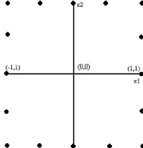
The forward method is used in this example. As shown in Fig.1, 16 points are chosen as initial condition
where (0) 1
1 = j
x , j=1, 2,..., 16.
A-1- Approximation of Lyapunov Function by Polynomial Neural Network
As we know, algebraic polynomials are universal approximators [9]. Also a quadratic function is an appropriate Lyapunov candidate for many groups of dynamic system [5], [10], [11]. Therefore polynomials can approximate or construct a Lyapunov function. So we choose a quadratic polynomial function with unknown coefficients
as a candidate for Lyapunov function.
V(x) = a1x12+a2x22+a3x1x2 (4-2) where ai ,1 ≤ i ≤ 3 , is an unknown coefficient which is determined during learning. Decreasing rate of V(xk) describes as follows:
V(xk+1) = V(xk) – b*rand[0,1] (4-3)
where rand[0,1] is a random value with uniform distribution and b is a learning factor, 0<b<1. According to previous section, the forward algorithm is implemented. After 25 iterations, we have
0581 . 0
0144 . 1
807 . 0
3 2 1
− = = =
a a a
The obtained Lyapunov function and its time derivative are shown in figures 2 and 3, respectively.
Fig. 1.” ” denotes the location of initial conditions
Fig. 3. The time derivative of the constructed Lyapunov function
A-1- Approximation of Lyapunov Function by Sigmoidal Neural Network
In this case, the training data is chosen like previous section. The network is consisted of one hidden layer and 10 nodes in it. After 25 iterations, the approximation of Lyapunov function is obtained. Since obtaining the closed form of the calculated function is difficult, if the number of initial conditions have selected enough then the neural network gives local generalization [9], therefore V(x) in the vicinity of the training data is approximated correctly. Figure 4 indicates the approximate Lyapunov function. The behaviors of V(x) for three state trajectories of the system are shown in figures 5 through 7.
Fig. 4. The approximate Lyapunov function for the system (4-1)
Fig. 5. The approximate Lyapunov function trajectory for initial condition (-1,1)
Fig. 6. The approximate Lyapunov function trajectory for initial condition (0,-1)
Fig. 7. The approximate Lyapunov function trajectory for initial condition (-1,0)
B.Example 2
In this example the backward method and polynomial neural network are used to generate a Lyapunov function for the following system.
) sin( 2
) sin(
) sin(
3 2
1 3
3 2
3 1
1
x x
x x
x x
x x x
− + − =
− =
+ − =
& & &
(4-4)
Around the origin 26 points are selected as initial conditions such that 0 =1
∞ j
x . Consider the following quadratic function as a candidate Lyapunov function:
V(x) = a1x12+a2x22+a3x32+a4x1x2+a5x1x3+a6x2x3 (4-5) where ai ,1 ≤ i ≤ 6 , is an unknown coefficient which is determined during learning. The following negative definite function is considered as a desired time derivative of Lyapunov function V&d(x)
x x
x
Vd T
⎥ ⎥ ⎥
⎦ ⎤
⎢ ⎢ ⎢
⎣ ⎡
− − − =
120 0
0
0 150 0
0 0 100 )
(
&
a1 = 8.2021 a2 = 29.0620 a3 = 25.4311
a4 = -23.5342 a5 = -5.5971
a6 = -16.3772
We can easily check that the trained network is a Lyapunov function for the system (4-4). Therefore the origin of the system is asymptotically stable.
V.CONCLUSION
In this paper two algorithms have been proposed to construct a Lyapunov function based on approximation theory and the abilities of artificial neural networks. As we know, neural networks found wide application in many fields, both for function approximation and pattern recognition. However, in this study with considering some assumptions the network solved a problem subject to a few conditions which showed potentials of neural network for solving inequalities.
REFERENCES
[1] D.V. Prokhorov, “A Lyapunov machine for stability analysis of nonlinear systems,” IEEE International Conference on Neural Networks, Orlando, FL, USA, Vol. 2, pp. 1028-1031, 1994.
[2] G. Serpen, “Empirical Approximation for Lyapunov Functions with Artificial Neural Nets,” Proc. of IJCNN, Montreal, Canada, pp.735-740, July 31-Aug. 2, 2005.
[3] D. V. Prokhorov, L. Deldkamp, “Application of SVM to Lyapunov Function Approximation,” Proc. of the IJCNN, Washington DC, Vol. 1, pp. 383-387, 1999.
[4] A. Papachristodoulou, S. Prajna, “On the Construction of Lyapunov Functions Using Sum of Squares Decomposition,” Proc. of IEEE Conference on Decision and Control, 2002.
[5] V. Petridis, S. Petridis, “Construction of Neural Network Based Lyapunov Functions,” Proc. of the IJCNN, Vancouver, BC, Canada, July 16-21, pp. 5059-5065, 2006.
[6] D. V. Prokhorov, L. Deldkamp, “Analysing for Lyapunov Stability with Adaptic Critics,” Proc. of IEEE Conference on Systems, Man and Cybernetics, San Diego, pp. 1658-1661, 1998.
[7] N. E. Barabanov, D. V. Prokhorov, “A New method for Stability Analysis of Non-linear Discrete-Time Systems,” IEEETransactionson AutomaticControl, Vol. 48, pp. 2250-2255, 2003.
[8] H.K. Khalil, Nonlinear Systems. 2nd ed. Prentice Hall. Englewood Cliffs, NJ. 1996, ch. 3.
[9] J. A. Farrell, M. M. Polycarpou, Adaptive Approximation Based Control: Unifying Neural, Fuzzy and Traditional Adaptive Approximation Approaches, John Wiley & Sons, Inc. 2006, ch. 2. [10] H. Bouzaouache, N. B. Braiek, On the Stability Analysis of Nonlinear
Systems using Polynomial Lyapunov Functions, Mathematics and Computers in Simulation (2007), to be accepted.