Aprendizado multi-objetivo deredes RBF e de Máquinas de kernel

(1)

Illya Kokshenev

Aprendizado Multi-objetivo de

Redes RBF e de M´

aquinas de Kernel

(2)

Aprendizado Multi-objetivo de

Redes RBF e de M´

aquinas de Kernel

Tese apresentada à banca examinadora designada pelo Colegiado do Programa de Pós-Gradua¸cão em Engenha-ria Elétrica da Universidade Federal de Minas Gerais,

como parte dos requisitos necessários à obten¸cão do grau de doutor em Engenharia Elétrica.

Orientador: Prof. Dr. Antˆonio P. Braga

(3)

Avan¸cos recentes em aprendizagem de máquina contemplam ampla variedade de tarefas de inteligência computacional, que têm sido aplicadas em vários problemas modernos de engenharia, economia, biomedicina, dentre outros. Tarefas como reco-nhecimento de padrões, previsão de séries temporais, controle adaptativo e deteçcão de falhas podem ser formuladas em termos da busca de dependências escondidas em observa¸cões emp´ıricas. Tal busca desempenha um papel central no contexto de apren-dizagem de máquina, e corresponde ao problema de aprenapren-dizagem supervisionada.

Considerando que as observa¸cões emp´ıricas são geralmente induzidas por variáveis de entrada não observadas, cujas propriedades são desconhecidas, a aprendizagem supervisionada deve ser tratada como um processo não-determin´ıstico nas condi¸cões de incerteza. Isto, por sua vez, faz com que o complexo metodológico da aprendizagem de máquina seja difundido para outros campos, tais como estat´ıstica, programa¸cão matemática, teorias de informa¸cão e tomada de decisões.

Uma visão abrangente do problema de aprendizagem supervisionada é dada pela teoria de aprendizagem estat´ıstica (SLT) [Vapnik, 1998], que estabelece os princ´ıpios de minimiza¸cão emp´ırica e estrutural do risco (ERM e SRM, correspondentemente). A implementa¸cão destes princ´ıpios encontra-se nos bem conhecidos conceitos de apren-dizagem, tais como redes de regulariza¸cão [Poggio and Girosi, 1990] e aprendizagem Bayesiana [Neal, 1996], cuja combina¸cão com as máquinas de vetores de suporte (SVM) [Cortes and Vapnik, 1995] e métodos de kernel modernos [Scholkopf, 1999] representam o estado da arte em aprendizagem de máquina.

Com o recente desenvolvimento da otimiza¸cão evolucionária, tem havido crescente interesse na aplica¸cão do conceito dePareto-optimality para estender as capacidades dos algoritmos e modelos aprendizagem. Esses conceitos tem sido aplicados no desen-volvimento de métodos de aprendizagem de máquina multi-objetivo (MOML) [Jin, 2006], em que a aprendizagem é considerada como um processo de tomada de decisão no ambiente de múltiplos critérios conflitantes.

Do ponto de vista multi-objetivo, a aprendizagem supervisionada pode ser repre-sentada como um problema de tomada de decisão entre dois objetivos conflitantes: minimiza¸cão de erro de treinamento (risco emp´ırico) e complexidade de modelo. Den-tro da abordagem tradicional (mono-objetivo), este processo corresponde à sele¸cão de modelos pelo princ´ıpio SRM. Esta visão quanto ao problema de aprendizagem supervisionada apresenta-se como o objeto de pesquisa deste trabalho.

A presente tese foi estruturada a partir de seis cap´ıtulos e três apêndices que apre-sentam uma introdu¸cão do tema, uma análise sistemática dos fundamentos teóricos conhecidos, desenvolvimento da metodologia proposta, suas aplica¸cões e resultados dos testes realizados, além das conclusões finais.

(4)

As máquinas de aprendizagem modernas, tais como SVM, são baseadas no princ´ıpio de regulariza¸cão e, portanto, representam problemas convexos cujas solu¸cões únicas podem ser obtidas de maneira eficiente por meio da programa¸cão não-linear. Entre-tanto, suas extensões aos mais amplos espa¸cos de hipóteses (e.g., com introdu¸cão de parâmetros de kernel), tradicionalmente, são efetuadas no n´ıvel de sele¸cão de modelo através de uma busca no espa¸co de múltiplos hiper-parâmetros. Essa abordagem de extensão, no entanto, não corresponde ao princ´ıpio de SRM, que apresenta-se como uma busca unidimensional de equil´ıbrio entre o erro e complexidade de mo-delo. Por outro lado, a extensão correspondente ao princ´ıpio de SRM é poss´ıvel com a abordagem multi-objetivo. Entretanto, devido a não-convexidade dos problemas de otimiza¸cão associados, que são NP-completos, a aplica¸cão de técnicas de solu¸cões aproximadas de programa¸cão global é requerida. Este fato explica porque a maioria das solu¸cões propostas da área MOML (e.g., [Liu. and Kadirkamanathan, 1995; Ha-tanaka and Uosaki, 2003; Jin, Okabe, and Sendhoff, 2004; Bevilacqua, Mastronardi, Menolascina, Pannarale, and Pedone, 2006; Yen, 2006; Kondo, Hatanaka, and Uosaki, 2006]) são orientadas para as técnicas de otimiza¸cão evolucionária, prestando pouca aten¸cão à implementa¸cão dos princ´ıpios fundamentais de aprendizagem estat´ıstica.

Como alternativa, nos trabalhos [Teixeira, Braga, Takahashi, and Saldanha, 2000; Costa, Braga, Menezes, Teixeira, and Parma, 2003; Costa and Braga, 2006] foi de-senvolvida a abordagem chamada MOBJ, para a aprendizagem multi-objetivo das redes perceptron de múltiplas camadas (MLP). Neste caso, com o objetivo de con-trole da generaliza¸cão conforme [Bartlett, 1997], o erro de treinamento foi minimizado junto com a norma Euclidiana dos pesos de rede através das técnicas de programa¸cão linear de maneira determin´ıstica (evolucionária). Contudo, devido a não-convexidade do problema tratado, a abordagem MOBJ desenvolvida nos trabalhos supracitados pode apresentar solu¸cões fracamente não-dominadas.

Conforme os resultados publicados, ambas as abordagens de multi-objetivo (evo-lucionária e MOBJ) demonstram um bom potencial, enquanto a conexão com SRM e utiliza¸cão das capacidades de programa¸cão não-linear mostram as vantagens do MOBJ. Então, sua certa evolu¸cão em dire¸cão à garantia de Pareto-optimality de solu¸cões e a implementa¸cão de SRM determina um caminho de desenvolvimento para uma nova abordagem eficiente.

Por apresentar fundamentos teóricos associados com máquinas de kernel e regu-lariza¸cão, as redes de fun¸cões da base radial (RBF) foram escolhidas para o desen-volvimento dos novos conceitos, métodos, e modelos de aprendizagem multi-objetivo neste trabalho.

(5)

conceito unificado.

Do ponto de vista estat´ıstico, dada uma fun¸cão de perda l(x, y, f(x)) como uma medida de erro de classifica¸cão ou regressão, e o conjunto deN observa¸cões

ZtrN :=

{

(xi, yi)∈ X × Y |i= 1. . . N }

,

i.i.d. de acordo com a distribui¸cão desconhecidaP(x, y), o problema de aprendizagem supervisionada é formulado como minimiza¸cão do funcional de risco esperado

R[f] := ∫

X ×Y

l(x, y, f(x))∂P(x, y) = E[l(x, y, f(x))], (1) sobre o espa¸co de hipóteses Ω. O espa¸co Ω representa uma classe de fun¸cões f : X → Y, suportadas pela máquina de aprendizagem, que mapeiam as observa¸cões do dom´ınio entrada_X para dom´ınio de sa´ıda_Y. Devido a indisponibilidade deP(x, y), o funcional (1) não pode ser minimizado diretamente, mas somente a sua aproxima¸cão emp´ırica

Remp[f] :=

1

N

N ∑

i=1

l(xi, yi, f(xi)), (2)

dispon´ıvel atrav´es do conjunto de observa¸c˜oes ZN

tr. Entretanto, conforme [Vapnik

and Chervonenkis, 1989], a minimiza¸cão do (2) que corresponde ao princ´ıpio de mi-nimiza¸cão do risco emp´ırico (ERM), leva a uma estima¸cão consistente do m´ınimo do risco esperado somente quando a convergência de Remp[f] para R[f] é uniforme,

assumindo a condi¸cão de que a capacidade da classe Ω seja limitada. Como mostra o resultado de análise da convergência, existe um limite superior do risco esperado na forma

R[f]_≤Remp[f] + Ψ (Remp[f], N,Ω, η) (3)

onde Ψ determina o intervalo de confian¸ca que se mantém com a probabilidade maior do que 1−η. É poss´ıvel demonstrar que o risco emp´ırico é uma fun¸cão decrescente da capacidade de Ω, e crescente para o intervalo de confian¸ca (o mesmo fenômeno é conhecido como o dilema bias-variance [Geman, Bienenstock, and Doursat, 1992]). Então, existe um espa¸co Ω de certa capacidade que garante o menor risco esperado através do limite (3). Esta idéia constitui a base do princ´ıpio indutivo de minimiza¸cão estrutural do risco (SRM), que considera a constru¸cão de uma estrutura de conjuntos aninhados,

∅ ⊂Ω1 ⊂Ω2 ⊂. . .⊂Ω

(6)

cuja complexidade leva ao menor risco emp´ırico, sendo este garantido por seu limite superior. Desta maneira, o problema de aprendizagem supervisionado é visualizado como uma busca de equil´ıbrio entre o m´ınimo de risco emp´ırico (menor erro de trei-namento) e menor capacidade de espa¸co de hipóteses de máquina de aprendizagem (complexidade do modelo).

´

E poss´ıvel mostrar que o problema do aprendizado supervisionado, tratado como um problemaill-posed com o método de regulariza¸cão [Tikhonov, 1943], corresponde à implementa¸cão do princ´ıpio de SRM na forma de minimiza¸cão do funcional risco regularizado

Rreg[f] :=Remp[f] +λQ[f], (4)

ondeQ[f] =_∥Df_∥2 _{´e o termo estabilizador (regularizador) baseado em um operador}

linear diferencialD, eλé o parâmetro da regulariza¸cão. Como foi mostrado em [Pog-gio and Girosi, 1990] e [Scholkopf, Herbrich, Smola, and Williamson, 2001], no caso mais geral, o m´ınimo global de (4) está contido no espa¸co de Hilbert do kernel re-produtivo [Aronszajn, 1950] (RKHS) Hk. Os elementos do RKHS são fun¸cões que admitem uma expansão

f(x) =∑ i

αik(x, xi), ₍₅₎

onde

k(x, x′) := ⟨Φ(x),Φ(x′)⟩=⟨ex,ex′⟩

é a fun¸cão de kernel definido positivo, correspondente ao produto escalar das imagens de seus argumentos através de um mapeamento não-linear Φk:X → Hk, e associada com operador autoadjuntoDDe como sua fun¸cão de Green. Assim, o termoQatravés do operadorDunicamente determina o kernelk e seu espa¸co RKHS Hk associado de fun¸cões (5). É poss´ıvel mostrar que as fun¸cões (5) podem ser evolu´ıdas como produto escalar

f(x) =⟨k(x,·), f⟩Hk (6)

em RKHS ou na forma geral

f(x) = ⟨x,_e fe⟩ (7)

em qualquer outro espa¸co de Hilbert, isom´orfico ao _Hk, onde e

f :=∑

i

αixei,

(7)

Isto, por sua vez, permite uma extensão dos algoritmos e modelos lineares de apren-dizado a uma ampla variedade de fun¸cões não-lineares de maneira eficiente através de kernels.

Assim, a escolha do kernel corresponde à determina¸cão do espa¸co caracter´ıstico para uma máquina de aprendizagem linear. No ponto de vista da regulariza¸cão, a penaliza¸cão por termo regularizador Q implica a suavidade da fun¸cão através das propriedades espectrais do operador D, garantindo a solu¸cão única do problema com a restri¸cão de capacidade do conjunto de hipóteses. No espa¸co caracter´ıstico _Hk ou outro espa¸co de Hilbert isomórfico dele, o termo

Q[f] =_∥Df_∥2 =_∥fe_∥2 =_∥f_∥2_k

também corresponde ao quadrado de comprimento do vetor normal fedo hiperplano de separa¸cão, determinando o inverso de margem geométrica dele. Desta forma, a regulariza¸cão se relaciona com o conceito de maximiza¸cão da margem, que é uma base da classe de algoritmos, bem-conhecidos como SVM [Cortes and Vapnik, 1995]. Na interpreta¸cão Bayesiana de minimiza¸cão do risco regularizado (4), a escolha da fun¸cão de perdal(x, y, f(x)), o valor do parâmetro de regulariza¸cãoλ, e o termoQ[f] (chamado de prior) correspondem ao fornecimento de informa¸cões a priori sobre o modelo de ru´ıdo, sua variância, e distribui¸cão de probabilidade das hipóteses [Girosi, Jones, and Poggio, 1993], respectivamente. Assim, considerando uma escolha a priori de l(x, y, f(x)) e Q[f] (ou seu correspondente kernel k) a solu¸cão do problema de aprendizagem pela minimiza¸cão de (4) pode ser unicamente determinada pelo escolha deλ como

fλ = KM(ZtrN, Remp, λQ[·]), (8)

onde KM ´e o resultado de um algoritmo de kernel gen´erico que fornece o extremo de (4) dado um conjunto de treinamento ZN

tr e os termos Remp e Q. Desta maneira,

o problema se reduz à estima¸cão do hiper-parâmetro λ pelo processo de sele¸cão de modelo

λ = arg min

λ∈R+ζ(fλ) (9)

através de um critérioζ, que também corresponde a implementa¸cão de princ´ıpio SRM quando ζ é uma estimativa do risco esperado.

Devido `a incerteza associada com Remp e Q, de maneira geral, as suas escolhas

s˜ao efetuadas junto com λ atrav´es de uma busca estendida (θR, θQ) = arg min

(θR,θQ)∈Θ

ζ(fθR,θQ

)

(10)

(8)

a hip´otese estendida na forma

fθR,θQ = KM(Z

N

tr, Remp_θ_R[·], QθQ[·]),

semelhante a (8). Na pr´atica, ´e comum escolher l(x, y, f(x)) empiricamente, quando

λe os hiperparâmetros de Q(que são os parâmetros de kernel) são estimados através de (10). Neste caso, somente o processo da estima¸cão de λ corresponde à escolha da capacidade do espa¸co de hipóteses de uma estrutura aninhada em Hk induzida com

Q, que corresponde a uma implementa¸cão do SRM, enquanto a estima¸cão dos hiper-parâmetros do priorQ é considerada como um n´ıvel de inferência mais alto [Guyon, Saffari, Dror, and Cawley, 2010].

Por outro lado, a parametriza¸cão do prior pode ser considerada como uma extensão do espa¸co de hipóteses da máquina de aprendizagem ao conjunto de múltiplos RKHSs onde, conforme princ´ıpio SRM, somente uma busca unidimensional é necessária para determinar o equil´ıbrio entre o risco emp´ırico e complexidade do modelo. Assim, a busca (10) é considerada redundante cujo espa¸co pode ser reduzido, reduzindo também a incerteza do problema de aprendizagem. Isto levará ao aumento de con-fian¸ca dos parâmetros estimados e, como sua conseqüência, o aumento de qualidade da generaliza¸cão obtida. Este ponto justifica a necessidade de desenvolvimento dos novos métodos e modelos de aprendizagem.

OCap´ıtulo 3introduz os conceitos básicos de otimiza¸cão multi-objetivo e deter-mina os elementos principais da abordagem desenvolvida, tais como formula¸cão do problema de otimiza¸cão e o método determin´ıstico da sua solu¸cão.

Visualizando o problema de aprendizado supervisionado como um processo de decisão multicritério, é poss´ıvel formular um procedimento geral para solu¸cão do problema de acordo com o esquema seguinte: avaliar o conjunto de todas alternativas Pareto-ótimas e tomar decisão de escolha de um único elemento. O primeiro passo corresponde à redu¸cão da região de incerteza do dom´ınio do problema que, no caso de objetivos conflitantes, representa o trade-off: aumento do n´ıvel de satisfa¸cão de um objetivo exige a redu¸cão do n´ıvel de satisfa¸cão do outro.

No contexto de SEM, em dom´ınio de um RKHS_Hk, os objetivos conflitantes s˜ao o risco emp´ıricoRemp e o priorQ(que desempenha o papel da medida de complexidade

do modelo), enquanto a regi˜ao do trade-off corresponde ao conjunto Pareto [Pareto, 1896] do problema de minimiza¸c˜ao bi-objetivo

min f∈Hk

ϕ[f] = (Remp[f], Q[f]), (11)

onde ϕ´e o vetor-funcional minimizado.

(9)

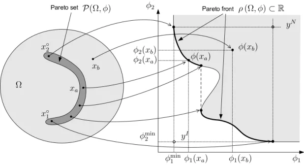
P(Ω, ϕ) :={x∈Ω| ∀x′ ∈Ω : x≼ϕ x′}, (12)

onde a rela¸cão x _≼ϕ x′ _{significa “}_x _domina _x′ _{com rela¸cão a} _ϕ_{” e corresponde à uma}

rela¸c˜ao de ordem lexicogr´afica das imagens dex e x′ sobre ϕ.

No contexto do problema bi-critério (11), é poss´ıvel mostrar que obten¸cão dos elementos Pareto-òtimos_P(_Hk, ϕ) pelo método de soma ponderada [Geoffrion, 1968] equivalente a minimiza¸cão do risco regularizado (4) para os todos valores deλ_∈R+_,

enquanto a decisão correspondente ao m´ınimo deζemP(Hk, ϕ) é equivalente a sele¸cão de modelo na forma (9). Na mesma maneira, é poss´ıvel superar a desvantagem da busca estendida (10) com a abordagem multi-objetivo, implementando o princ´ıpio de SRM em um espa¸co de hipóteses estendido de múltiplos RKHSs com uma busca dentro do correspondente conjunto Pareto.

Especialmente, introduzindo uma fam´ılia de kernels

K ⊂{k∈RX2}

ao seu correspondente espa¸co de hip´otese HK :=

∪

k∈K

Hk, (13)

induzido pela uni˜ao dos associados RKHSs, ´e poss´ıvel substituir (10) com o procedi-mento multi-objetivo

fmobj= arg min

f∈P(HK,ϕ)

ζ[f], (14)

que corresponde à uma máquina de aprendizagem com a capacidade de escolha de kernel (e seus hiperparâmetros) implementando o princ´ıpio de SRM. A forma proposta de solu¸cão do problema de aprendizagem pode considerada como uma evolu¸cão da abordagem chamado MOBJ, desenvolvida nos trabalhos recentes [Teixeira, Braga, Takahashi, and Saldanha, 2000; Costa, Braga, Menezes, Teixeira, and Parma, 2003; Costa and Braga, 2006].

Contudo, para colocar a abordagem MOBJ proposta em (14) na prática, é ne-cessário resolver dois problemas.

Primeiramente, precisa-se definir certa medida de complexidade Q no espa¸co es-tendido _HK. Infelizmente, como ´e demonstrado neste trabalho, para um caso geral de fam´ılia de kernelsK, a medida de complexidade n˜ao pode ser um prior e, por isso,

(10)

ao seu resultado independente.

Em seguida, é necessário desenvolver um método de obten¸cão das hipóteses Pareto-ótimasP(HK, ϕ) de uma forma determin´ıstica. Devido à não-convexidade do dom´ınio HK e, conseqüentemente, do problema multi-objetivo, a sua solu¸cão não pode ser ob-tida pela aplica¸cão do método de soma ponderada cuja aplica¸cão é adequada somente para problemas estritamente convexos [Das and Dennis, 1997]. Contudo, a aplica¸cão do método ϵ-restrito [Haimes, Lasdon, and Wismer, 1971; Chankong and Haimes, 1983] é poss´ıvel, mas não eficiente devido à necessidade de busca dos m´ınimos glo-bais. Então, como solu¸cão foi proposto um método de decomposi¸cão dos conjuntos não dominados que permite decompor o problema MOBJ em conjunto de sub-problemas convexos na forma,

P(_HK, ϕ) =P (

∪

k∈K

P(_Hk, ϕ), ϕ )

, (15)

que possibilita reconstruir o conjunto Pareto_P(_HK, ϕ) no dom´ınio global através dos conjuntos não-dominados P(Hk, ϕ), k ∈ K cujos elementos podem ser obtidos pela programa¸cão convexa minimizando uma certa forma de (4). Na prática, aproximando

K com o número finito de elementos, o método de decomposi¸cão permite gerar um subconjunto finito de hipóteses Pareto-ótimos P(HK, ϕ) em um tempo garantido na forma determin´ıstica.

Assim, a abordagem proposta pode ser considerada como um conceito generali-zado de aprendizagem supervisionada para uma classe geral de máquinas de kernel na forma de um algoritmo MOBJ, baseado em procedimento de sele¸cão de modelo multi-objetivo (14) que implementa o princ´ıpio SRM dado uma certa medida de com-plexidade, e cujos resultados podem ser obtidos de maneira eficiente e determin´ıstica através da decomposi¸cão (15).

NoCap´ıtulo 4, a medida de complexidade proposta ´e baseada no conceito de sua-vidade que, em combina¸c˜ao com a abordagem MOBJ desenvolvida, leva ao algoritmo de aprendizagem para redes RBF.

Em regulariza¸cão, a complexidade da hipótese é refletida pelo termo regularizador, que no dom´ınio Fourier corresponde ao filtro de passa-alta, implicando certo grau de suavidade à fun¸cãof. A suavidade de uma fun¸cão, no entanto, pode ser determinada de maneira expl´ıcita, fora do contexto do regularizador (prior, ou seu correspondente kernel). Uma medida de complexidade pode ser obtida para o espa¸co de hipóteses arbitrário, inclusive para _HK induzido por uma fam´ılia K.

(11)

i=1

onde ci s˜ao os centros das fun¸c˜oes RBF kσ(x, ci) = kσ(x−ci) = κ(x−_σci) de largura

σ. Em particular, ´e mostrado que a norma _∥f_∥q,p no espa¸co de Sobolev Wq,p possui o limite superior

∥f∥q,p ≤ ∥α∥1· ∥kσ∥q,p, (16)

ondeα= (α1, α2, . . . , αm)T ´e o vetor de coeficientes da expans˜ao (pesos) da rede RBF

correspondente aof. Baseado em uma modifica¸c˜ao de (16), a medida de complexidade

Qrbf[f] = σ−

n

p∥α∥

1

∑

|s|=q ∥Ds_k

σ∥p, (17)

foi proposta, onde

Ds := ∂

|s|

∂xs1

1 ∂x

s2

2 · · ·∂xsnn ´e o operador diferencial generalizado sobre o espa¸co RRn

, dado pelo multi-´ındice

s_∈Zn_.

Supondo que as fun¸cões kσ são Gaussianas, i.e., κ(u) = exp(−1₂∥u∥2), e a or-dem do diferencial da norma de Sobolev q = 2, é poss´ıvel mostrar que a medida de complexidade (16) se reduz à forma simples

Qrbf[f] = ∥

α_∥1

σ2 . (18)

Tal forma permite descrever o problema de aprendizagem MOBJ no espa¸co de hip´oteses

F :={f :Rn

→R|f(x) =∑ i

αikσ(x−ci) }

, (19)

correspondente a todas as poss´ıveis redes RBF com m _∈ N fun¸c˜oes bases, centros

ci ∈ Rn, larguras σ ∈ R+ e pesos αi ∈ R. Para obter uma aproxima¸c˜ao finita do conjunto Pareto

P(F, ϕ), ϕ[f] = (Remp[f], Qrbf[f]) (20)

de maneira eficiente, a redu¸c˜ao do dom´ınio F ao e

F = ∪

σ∈Sσ

Fσ,CM,

foi proposta, ondeFσ,CM s˜ao os elementos deF associados `as redes RBF cujos centros

correspondem a padr˜oes distintos do conjunto de treinamento. Assim, aplicando a

(12)

P(F , ϕe )=_P ∪ σ∈Sσ

P(Fσ,CM, ϕ), ϕ , (21)

onde Sσ = (σj)_j ´e um grid de larguras, cuja quantidade de elementos determina a qualidade da aproxima¸c˜ao de (20).

Como as estruturas (camadas escondidas) das redes RBF associadas com Fσ,CM

são iguais, o problema de busca dos elementos não-dominados_P(Fσ,CM, ϕ) é convexo.

Assumindo uma fun¸c˜ao de perda quadr´atical(x, y, f(x)) = (y−f(x))2_{, este problema}

pode ser resolvido no dom´ınio RM _minimizando

Rreg(α) = ∥Y −Hα∥2+λ∥α∥1, (22)

ondeY = (y1, y2, . . . , yN)T ´e o vetor das sa´ıdas desejadas do conjunto de treinamento

ZN

tr e H = {kσ(xi, cj)}, i = 1, . . . , N, j = 1, . . . , M ´e a matriz N ×M da camada escondida.

Sabe-se que (22) correspondente à regressão LASSO [Tibshirani, 1996], cujas solu¸cões são esparsas e seu caminho de regulariza¸cão (minimizadores de (22) cor-respondentes a todos λ _∈ R+_{) é uma curva linear em trechos no} _RM_{. O caminho} de regulariza¸cão do LASSO, que no contexto do presente problema representa o con-junto não-dominado _P(Fσ,CM, ϕ), pode ser inteiramente calculado através do

algo-ritmo LARS [Efron, Hastie, Johnstone, and Tibshirani, 2004]. Assim, a aproxima¸cão do conjunto Pareto (20) pode ser obtida diretamente de (21) através dos correspon-dentes resultados de múltiplas execu¸cões do LARS. Assim, a utiliza¸cão do conjunto (21) em um esquema (14) da abordagem MOBJ, levou ao algoritmo MOBJ-RBF de-senvolvido, que é capaz de determinar os pesos, larguras, centros e quantidades de fun¸cões-bases das redes RBF de acordo com principio SRM.

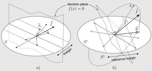
Em combina¸cão com os critérios de informa¸cão AIC [Akaike, 1974] e BIC [Schwarz, 1978], adaptados para sele¸cão de modelo no contexto de regressões LASSO, o algo-ritmo proposto demonstrou alto desempenho de generaliza¸cão para diversos proble-mas comumente usados comobenchmark.

OCap´ıtulo 5apresenta uma extensão multi-objetivo do conceito de maximiza¸cão da margem para o contexto do espa¸co de hipóteses _HK, associado aos múltiplos RKHSs.

Como foi mostrado na análise préliminar do problema, a escolha da medida de complexidade em _HK como o prior Q[f] =∥f∥2k (relacionado com a largura da mar-gem geométrica num subespa¸co Hk correspondente), não é adequada para o caso de uma fam´ılia de kernels K arbitrária. Assim, os conjuntos aninhados

Ωi :={f ∈ HK | ∥f∥2

k ≤ϵi},

(13)

dependente da normaliza¸cão dos kernels emK, enquanto o espa¸co das fun¸cões, repre-sentadas por _HK, continua sendo independente. Desta maneira, a organiza¸cão de K

influencia o conjunto de hipóteses Pareto-ótimas sem influenciar suas propriedades da generaliza¸cão. Assim, _∥f_∥2

k n˜ao representa uma medida de complexidade adequada em HK.

Do ponto de vista dos espa¸cos de caracter´ıstica, a viola¸c˜ao do SRM com a escolha

Q[f] = _∥f_∥2

k é causada pelas diferen¸cas de suas topologias, que levam à incompati-bilidade das métricas. Assim, o problema pode ser resolvido por certa equipara¸cão dos espa¸cos. Especialmente, uma das técnicas de equipara¸cão desenvolvida é a nor-maliza¸cão dos tamanhos dos vetores caracter´ısticos, que leva à seguinte medida de complexidade normalizada

Qnorm[f] :=

∑

i ∑

j

αiαj √

k(xi, xi)k(xj, xj)k(xi, xj). (23)

No caso espec´ıfico, quando os vetores caracter´ısticos associados ao kernelk tˆem com-primentos iguais (e.g., como no caso de kernel RBF Gaussiano), o valor do Qnorm[f]

corresponde ao quadrado de norma RKHS de uma hip´otese f′_{, cujo kernel induz}

ve-tores caracter´ısticos unit´arios, equivalente ao f. No caso do kernel geral, a hip´otese

f′ _{n˜ao necessariamente ´e equivalente a} _f_{, mas a medida} _Q

norm[f] ´e invariante aos

escalamentos dos espa¸cos de caracter´ıstica associados comf.

De fato, é poss´ıvel demonstrar que a capacidade do espa¸co RKHS é influenci-ada não somente pelos comprimentos de vetores caracter´ısticos, mas também pela sua topologia angular. Por exemplo, é fácil verificar que os kernels suaves induzem vetores caracter´ısticos fracamente angulados. Assim, a equipara¸cão dos espa¸cos de caracter´ıstica a partir da normaliza¸cão dos vetores caracter´ısticos pode não ser sufi-ciente para representar as complexidades das hipóteses na forma adequada. Por isso, foi proposta outra abordagem de equipara¸cão, baseada na idéia de representar todas as hipóteses em único espa¸co de caracter´ısticas de forma equivalente. Esta técnica denominada equaliza¸cão, é formulada a partir do princ´ıpio a seguir.

Dado um mapeamento Φ◦ _:_{X → H}◦ _{fixo ao espa¸co de referˆencia} _H◦ _assumimos

que ´e poss´ıvel representar qualquer kernelk ∈K na forma do produto escalar emH◦

k(x, x′) =⟨Φ◦(x),Φ∗k(x′)⟩H◦ =⟨ ◦

x, ∗

x′⟩ para os todos (x, x′)∈ X2_, ₍₂₄₎

onde Φ∗

k(x′) :X → H◦ ´e um mapeamento auxiliar associado com k. Assim, qualquer hip´otesef _{∈ H}K pode ser representada na forma equivalente pelo produto escalar no

(14)

f(x) = x,f (25) atrav´es da sua imagem auxiliar

∗

f =∑

i

αi

∗

xi. (26)

Na forma da hipótese (7), ambos componentes do produto escalar são dependentes do mapeamento Φk. Em contrapartida, a forma equivalente (25) considera os ve-tores caracter´ısticos de referência ◦

x, independentes do kernel e comuns para todas as hip´oteses. Assim, os elementos _HK podem ser analisados num espa¸co de carac-ter´ısticas equalizado, com as suas propriedades expressas em termos das correspon-dentes imagens auxiliares

∗

f.

A análise do paradigma das hipóteses no espa¸co de referência mostrou que a margem geométrica do hiperplano de separa¸cão corresponde ao inverso do com-primento do vetor ◦

g, que representa a proje¸c˜ao ortogonal de

∗

f no espa¸co linear

S◦ _{:= span}_{◦

xi} N

i=1, gerado pelas combina¸c˜oes lineares dos vetores caracter´ısticos de

referˆencia. Por outro lado, foi demonstrado que a introdu¸c˜ao da medida de comple-xidade baseada na largura da margem, tal como ∥◦

g∥2 _ou _∥_f∗_∥2_{, leva a degenera¸c˜oes}

do espa¸co de hipóteses da máquina de aprendizagem e, por isso, não representa a escolha aceitável. Esta conclusão justificou a necessidade do desenvolvimento de uma extensão do conceito de margem geométrica a uma propriedade de hiperplano de separa¸cão mais geral.

Seguindo uma conhecida interpreta¸cão de margem larga como a estabilidade pa-ramétrica do modelo, o critério de estabilidade leave-one-out do hiperplano de se-para¸cão foi proposto. Particularmente, dado um hiperplano de sese-para¸cão pelo seu vetor normalf na forma da combina¸cão linear

f = N ∑

j=1

αjxj (27)

dos N vetores-suportexj, j = 1, . . . , N, a sua estabilidade ´e definida pelo crit´erio

E(f) := N ∑

i=1

e2_i, (28)

onde

e2_i =_∥f ₋g(i)

∥2 (29)

(15)

g(i) := ∑ j=1,j̸=i

βj(i)xj

considerando os N ₋1 vetores-suporte, após a exclusão do i-ésimo. A partir da transforma¸cão realizada, foi mostrado que o critério (28) possui a forma compacta

E(f) = N ∑

i=1

α2

i

di

, (30)

onde (d1, d2, . . . , dN) = diag(G−1) s˜ao os elementos diagonais do inverso da matriz de Gram G=XT_X_{, associada com os vetores-suporte} _X _{= (}_x

1, x2, . . . , xN). ´

E poss´ıvel mostrar, que o critério proposto (30) está diretamente ligado a norma ∥f∥2 _{(que reflete a largura da margem geométrica) e, além disso, considera o volume}

de informa¸cão mútua na descri¸cão do vetor f, no sistema de vetores-suporte dado por X. Desta forma, o critério (30) pode ser interpretado como uma medida de complexidade dentro do conceito de minimum description length (MDL) [Wallace and Boulton, 1968], sendo uma medida do volume de informa¸cão necessário para descri¸cão do modelo de um classificador, representado porf, com certa precisão.

Como o critério (30) também é dependente da métrica num espa¸co de Hilbert, as-sociado comf, a medida de complexidade baseada em (30) para o espa¸co de hipóteses HK exige a equipara¸cão dos correspondentes RKHSs. Assim, aplicando a técnica de equaliza¸cão desenvolvida, foi proposta a medida de complexidade de referência

Qref[f] :=

N ∑

i=1

α2

i

di

, (31)

que é baseada no critério de estabilidade do hiperplano de separa¸cão dos padrões em

S◦ _{associado com}_f _{∈ H}_{k. Em (31), os elementos diagonais}

(d1, d2, . . . , dN) = diag (

G−_k1Gk◦G−1

k )

s˜ao calculados a partir das matrizes de Gram G−_k1 e Gk◦, associadas com o kernel k

e o kernel de referˆencia k◦_{, respectivamente.}

O kernel de referênciak◦_{é associado com Φ}◦ _{através dos produtos escalares dos}

ve-tores caracter´ısticos ◦

xi. Por isso, a sua escolha influencia na medida de complexidade

Qref. Se por um lado, a escolha de um Φ◦ deve garantir a existˆencia dos mapeamentos

auxiliares Φ∗

k para todos os elementos da fam´ıliaK, fornecendo a possibilidade de re-presenta¸c˜ao equivalente de todas as hip´oteses emHK na forma (25); por outro lado,

(16)

dos mapeamentos auxiliares e a abordagem prática para suas deriva¸cões, inclusive nas formas fechadas dos kernels associados. Utilizando estes resultados, foi proposta a escolha universal de mapeamento de referência Φ◦ _{com o kernel}

k◦(xi, xj) = δji = {

1, i=j

0, se contr´ario

sendo a fun¸c˜ao delta de Kronecker, que leva a uma forma pr´atica de medidaQref para

qualquer _HK.

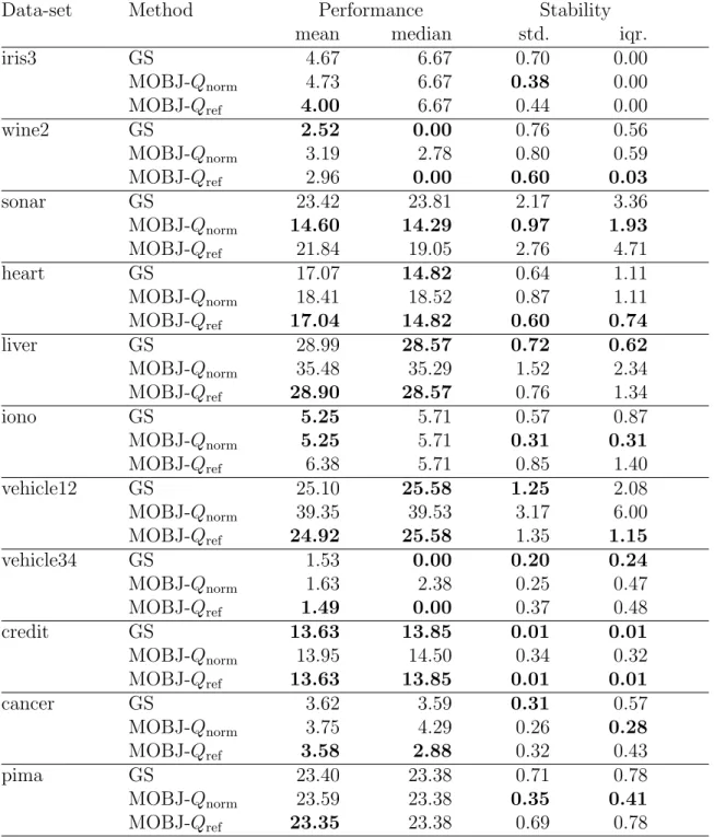
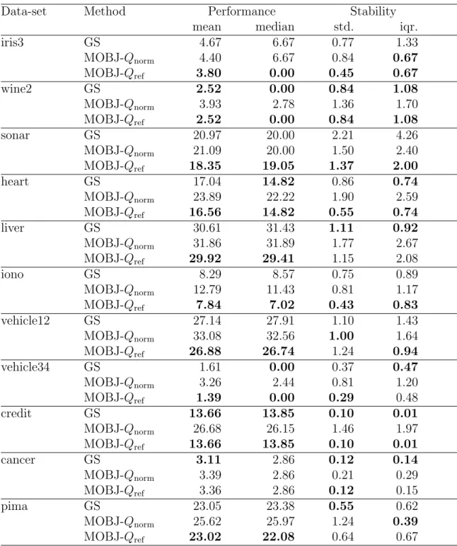
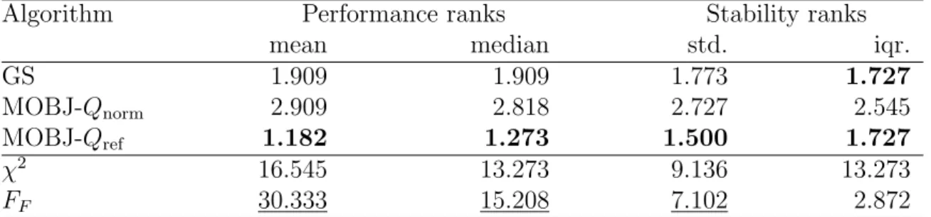
Para confirmar a adequa¸cão da abordagem desenvolvida, um algoritmo MOBJ no dom´ınio de solu¸cões de SVM, baseado no esquema (14) com as medidas de comple-xidade propostas (23) e (31) foi comparado com a busca (10) pelo grid equivalente, numa série de experimentos extensivos. A análise estat´ıstica dos resultados obtidos com experimentos confirmou as propriedades esperadas da medida Qref, juntamente

com a redundˆancia das buscas exaustivas (10) no espa¸co de hiperparˆametros, como foi teoricamente previsto no Cap´ıtulo 2. Este resultado justifica a necessidade de desenvolvimentos futuros da abordagem MOBJ.

O Cap´ıtulo 6 conclui o presente trabalho resumindo os resultados teóricos e práticos obtidos, junto com a discussão das perspectivas de desenvolvimentos futuros. Os resultados dos Cap´ıtulos 3 e 4 desse trabalho foram apresentados em con-gressos nacionais e internacionais, e também publicados em periódicos revisados. Os resultados de Cap´ıtulo 5 encontram-se em fase de prepara¸cão para submissão.

Produ¸c˜ao bibliogr´afica

I. Kokshenev and A. P. Braga. Complexity bounds of radial basis functions and multi-objective learning. Em ESANN, p´aginas 73–78, 2007.

I. Kokshenev and A. P. Braga. A multi-objective approach to RBF network learning.

Neurocomputing, 71(7-9):1203–1209, 2008a.

I. Kokshenev and A. P. Braga. A multi-objective learning algorithm for rbf neural network. Em 10th Brazilian Symposium on Neural Networks, SBRN 2008, p´aginas 9–14, 2008b.

I. Kokshenev and A. P. Braga. An efficient multi-objective learning algorithm for RBF neural network. Neurocomputing, 2010. (aceito)

(17)

Multi-objective Learning of Radial-Basis

Function Networks and Kernel Machines

Illya Kokshenev

A dissertation thesis submitted to the examination com-mittee in partial fulfillment of the requirements for the

degree of doctor in Electrical Engineering.

Supervisor: Prof. Dr. Antˆonio P. Braga.

(18)

(19)

Acknowledgements

I am most grateful to my supervisor, Antˆonio de Padua Braga, Dr., Professor of the Electrical Engineering Department and Head of the Computational Intelligence Lab-oratory (LITC) at the Federal University of Minas Gerais (UFMG), for his valuable guidance, advice, discussion, and support throughout this work.

I am gratefully indebted to Yevgeniy Bodyanskiy, Dr. Sci., Professor of the Arti-ficial Intelligence Department and Head of the Control Systems Research Laboratory (CSRL) at the Kharkiv National University of Radio Electronics, Ukraine. His wide knowledge and encouraging guidance have been of great value for me since my very first steps in science and during my bachelor’s and master’s graduation.

I owe my most sincere gratitude to Hani Camille Yehia, Dr., Professor and ex-Coordinator of the Post-Graduate Programme of the Electrical Engineering Depart-ment, Head of the Center for Research on Speech, Acoustics, Language and Music (CEFALA) at the UFMG, for his enthusiasm, openness and welcome in my applica-tion for doctorate programme.

My sincere thanks are due to Petr Ekel, Dr. Sci., Professor of the the Post-Graduate Programme of the Electrical Engineering Department at the Pontifical Catholic University (PUC) of Minas Gerais, for his heplful advice and support in a number of ways since my first days in Brazil.

I am thankful to many of my colleagues from LITC and CSRL for their enthusiasm in discussion of ideas, exchange of experience, and assistance.

I also thank the National Council for Scientific and Technological Development of Brazil (CNPq), for their generous financial support.

(20)

Abstract

As known from statistical learning theory, the training error and complexity of a model must be simultaneously minimized and yet certainly balanced for a valid gen-eralization. Modern learning algorithms, such as support vector machines, achieve this goal by means of regularization and kernel methods, whose combination provides possibilities for analysis and construction of efficient nonlinear learning machines.

In such algorithms, due to the non-convexity of the learning problem when the kernel is not fixed, the choice of the kernel is commonly addressed using sophisticated techniques of model selection, in a manner, different from the original idea of balance between the error and complexity. In contrast, the search of balance between the error and complexity in non-convex learning problems can be treated within the multi-objective framework, by viewing the supervised learning as a decision process in the environment of two conflicting goals. However, modern methods of multi-objective learning are focused on evolutionary optimization, paying a few attention to implementation of key learning principles.

This work develops a multi-objective approach to supervised learning as an exten-sion of the traditional (single-objective) concepts, such as regularization and margin maximization, to the cases of non-convex hypothesis spaces, induced with multiple kernels. In the proposed learning scheme, approximate solutions to generally non-convex problems are obtained from their decompositions into the subsets of non-convex subproblems, where the application of deterministic nonlinear programming is effi-cient. Aiming for implementation of the principle of structural risk minimization, there are several complexity measures derived, each one inducing a particular multi-objective algorithm.

In particular, the proposed smoothness-based complexity measure for the Gaus-sian radial-basis function (RBF) networks led to an efficient multi-objective algorithm, which is capable of finding the weights, widths, locations, and quantities of basis functions in a deterministic manner. In combination with the Akaike and Bayesian information criteria, the developed algorithm demonstrates a high generalization ef-ficiency on several synthetic and real-world benchmark problems. Aiming to extend the concept of margin maximization to supervised learning with multiple kernels, the techniques of feature normalization and equalization were proposed. The further analysis shows the necessity in extension of the concept of margin to the more general property of a separation hyperplane, such as its stability. As the result, the proposed stability-based complexity measure, which reliability has been experimentally con-firmed, allows a construction of multi-objective algorithms for arbitrary classes of kernels.

(21)

Resumo

Conforme a teoria de aprendizagem estat´ıstica, o erro de treinamento e a complexi-dade de modelos de aprendizado devem ser certamente equilibrados para uma genera-liza¸cão válida, além de serem minimizados. Os algoritmos de aprendizagem modernos, tais como máquinas de vetores de suporte, atingem esta meta por meio da regula-riza¸cão e dos métodos de kernel. A sua combina¸cão permite de maneira eficiente analisar e construir máquinas de aprendizagem não-lineares.

Nestes algoritmos, devido à não-convexidade do problema de aprendizagem quando o kernel não é fixo, a escolha do kernel é efetuada por meio das técnicas sofisticadas de sele¸cão de modelos, diferentemente da ideia original de equil´ıbrio entre o erro e a complexidade. Por outro lado, a busca de equil´ıbrio entre o erro e a complexidade de problemas não-convexos pode ser tratada de maneira multi-objetiva, considerando a aprendizagem supervisionada como o processo de decisão no ambiente de dois obje-tivos conflitantes. Contudo, métodos modernos de aprendizagem multi-objetiva são voltados à otimiza¸cão evolucionária, prestando pouca aten¸cão à implementa¸cão dos princ´ıpios fundamentais de aprendizagem estat´ıstica.

Neste trabalho foi desenvolvida uma abordagem multi-objetiva de aprendizagem supervisionada baseada na extensão dos conceitos tradicionais, tais como regula-riza¸cão e maximiza¸cão de margem, aos casos de espa¸cos de hipótese não-convexos, induzidos com múltiplos kernels. No esquema de aprendizagem proposto, as solu¸cões aproximadas dos problemas, geralmente não-convexos, sao obtidos por meio de certa decomposi¸cão em conjuntos de sub-problemas convexos, nos quais a programa¸cão não linear pode ser eficientemente aplicada de maneira determin´ıstica. Com o objetivo de implementa¸cão do princ´ıpio de minimiza¸cão do risco estrutural, várias medidas de complexidade foram propostas, induzindo os correspondentes algoritmos multi-objetivos.

Entretanto, a medida de complexidade baseada em suavidade para as redes de fun¸cão da base radial (RBF) permitiu a constru¸cão de um algoritmo multi-objetivo, com a sua capacidade de defini¸cão dos pesos, larguras, centros e quantidades de fun¸cões-bases. Em combina¸cão com os critérios de informa¸cão de Akaike e Bayes, o algoritmo proposto demonstrou um alto desempenho de generaliza¸cão em vários problemas-testes de natureza diversa. Com o objetivo de extensão do conceito de maximiza¸cão de margem ao aprendizagem supervisionada com múltiplos kernels, as técnicas de normaliza¸cão e equaliza¸cão dos espa¸cos de caracter´ısticas foram propos-tas. As suas análises mostraram a necessidade de formula¸cão de conceito de margem com uma caracter´ıstica mais geral de hiperplano de separa¸cão, tal como sua estabili-dade. Como resultado, a medida de complexidade baseada no critério de estabilidade desenvolvido, cuja adequa¸cão foi confirmada com experimentos, permite a constru¸cão de algoritmos multi-objetivos para as classes de kernel arbitrários.

(22)

Acknowledgements ii

List of Figures ix

List of Tables x

Abbreviations and symbols xi

1 Introduction 1

1.1 Motivation and goals . . . 2 1.2 Thesis outline . . . 5

2 Theoretical background 7

(23)

2.5 A big picture . . . 31 2.5.1 Unified learning framework . . . 31 2.5.2 Hyperparameters and model selection . . . 33 2.5.3 Validation techniques . . . 35 2.5.4 Overview of kernel selection techniques . . . 36 2.6 Discussion and further motivation . . . 37

3 Multi-objective learning 38

3.1 Introduction . . . 38 3.1.1 Principle of Pareto-optimality . . . 39 3.1.2 Basic scalarization techniques . . . 42 3.1.3 Overview of approximate methods . . . 43 3.2 MOBJ: bicriteria supervised learning . . . 44 3.2.1 Generalized learning concept . . . 44 3.2.2 Complexity measure and priors . . . 46 3.2.3 Method of convex decomposition . . . 47 3.3 Summary . . . 49

4 Multi-objective algorithm for RBF networks 51

(24)

4.5 Experiments . . . 71 4.5.1 Twin spiral . . . 72 4.5.2 Noised sinc regression . . . 75 4.5.3 Wisconsin breast cancer . . . 77 4.5.4 Abalone data-set . . . 80 4.5.5 Discussion . . . 82 4.6 Summary . . . 84

5 Multi-objective extension of margin maximization 85

5.1 Introduction . . . 85 5.1.1 Why _∥f_∥2

k is not a valid complexity measure on arbitrary hy-pothesis space? . . . 86 5.2 Feature normalization . . . 89 5.2.1 Effective support vectors . . . 90 5.2.2 Normalized complexity measure . . . 91 5.2.3 Radius/margin interpretation . . . 92 5.3 Feature equalization . . . 92 5.3.1 Reference and auxiliary maps . . . 93 5.3.2 A closer look at the reference space . . . 95 5.3.3 The concept of margin in a reference space: an extension is

(25)

5.7 Summary . . . 119

6 Conclusions 120

A Auxiliary kernels 122

A.1 Basic considerations . . . 122 A.2 Convolution kernels . . . 124 A.3 Polynomial kernels . . . 127 A.4 Universal reference map . . . 129 A.5 Summary . . . 130

B Proofs of some lemmas 131

B.1 Matrix inversion lemma: particular case . . . 131 B.2 Proof of lemma 5.4.1 (Diagonal elements of the Gram matrix inverse) 132

C Visualizations of the experiment results from Chapter 5 134

(26)

2.1 Demonstration of the non-trivial consistency principle of empirical risk minimization. . . 12 2.2 Illustration of the structural risk minimization principle . . . 16 2.3 Architecture of the RBF network . . . 17 3.1 Schematic illustration of the Pareto-optimality principle and relations

between the problem domain (left) and the objective space (right) on example of the following elements: xa is Pareto-optimal; xb is domi-nated; x◦

1 = arg minx∈Ωϕ1(x) and x◦2 = arg minx∈Ωϕ2(x) are the

ex-trema; yI _and _yN _{are the ideal and nadir points, respectively. . . .} ₄₁ 4.1 Schematic demonstration of the the LASSO regularization path (left)

and the corresponding Pareto front (right). . . 62 4.2 Twin spiral experiment 1: 194 samples. . . 73 4.3 Twin spiral experiment 2: 582 samples with noise. . . 74 4.4 Distribution of the values of model selection criteria along the Pareto

sets in experiments 1 (left) and 2 (right). . . 74 4.5 The fragments of Pareto fronts from the sinc experiment,

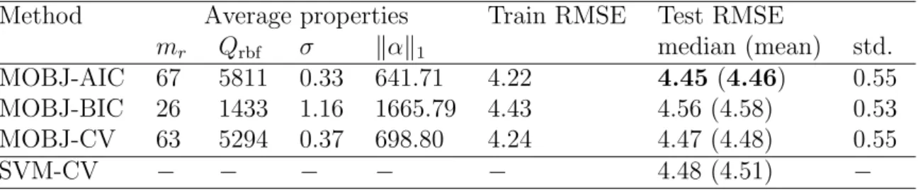
correspond-ing to a particular noise realization. . . 78 4.6 Experiment results for the Wisconsin breast cancer data-set. . . 81 5.1 Schematic representation of the hypothesis f in the conventional (a)

(27)

4.1 Twin-spiral benchmark results . . . 73 4.2 Results for the sinc regression benchmark: test NRMSE_×102 _(mean)

and its standard deviation (std.) . . . 77 4.3 Wisconsin breast cancer benchmark results . . . 80 4.4 Abalone data-set results: median values of solution parameters and

test RMSE . . . 81 5.1 List of the benchmark data-sets . . . 110 5.2 Selected ranges of hyperparameters . . . 112 5.3 Scores of GS, MOBJ-Qnorm and MOBJ-Qref with the Gaussian RBF

kernel on benchmark data-sets. . . 114 5.4 Scores of GS, MOBJ-Qnormand MOBJ-Qref with the polynomial kernel

(28)

Abbreviations

AIC Akaike information criterion ANN artificial neural network

BIC Bayessian information criterion CV cross-validation

GCV generalized cross-validation

GRN generalized regularization network i.i.d. independent and identically distributed

LASSO least absolute shrinkage and selection operator LARS least angle regression shrinkage

MAP maximum a posteriori probability MLP multilayer perceptron

MOBJ bi-objective supervised learning (concept, method, or algorithm) MOML multi-objective machine learning

MSE mean squared error

MVE minimum of validation error

NRMSE normalized root mean squared error OLS ordinary least squares

p.d.f. probability density function PCA principal component analysis RBF radial-basis function

RKHS reproducing kernel Hilbert space RN regularization network

(29)

SVM SV machine

SLT statistical learning theory SRM structural risk minimization

VC Vapnik-Chervonenkis (-dimension or -theory)

Important Symbols

b bias parameter

c usually a constant

ci center (prototype) of i-th basis function

D linear differential operator e

D adjoint of D

df[f] effective number of degrees of freedom of hypothesis f ei the i-th error, usually ei =yi−yˆi

E[x] expected value of random variable x

E(f) leave-one-out stability criterion (hyperplane error)

f(x) hypothesis, discriminant, or regression function e

f feature space representation of hypothesis f(x) =⟨x,e fe⟩

F hypothesis space and of RBF networks

F[κ](ω) Fourier transform of κ onRn

Gk Gram matrix associated with kernel k

G(x, xi) Green’s function to DDe

G(N) growth function, upper bound on Vapnik’s entropy

h VC-dimension

H design or kernel matrix

H Hilbert space

Hk RKHS associated with k

i index variable or imaginary unit

I identity matrix

k(·,·) kernel function

(30)

Lp space of p−integrable functions

m number of basis functions (hidden units) or support vectors

n dimensionality of input space

N number of training samples (length of the training set) N set of natural numbers

O(g(x)) asymptotic growth rate of g(x) (Bachmann-Landau notation) P(Ω, ϕ) nondominated or Pareto set of Ω w.r.t. ϕ

Pr_{X_} probability of event X

p(x, y) joint probability density function of distribution P(x, y)

P(x, y) joint probability distribution of random variables x and y Q[f] regularization stabilizer, prior, or complexity measure of f R[·] expected risk functional

R field of real numbers

R+ _{set of non-negative real numbers}

Remp[·] empirical risk functional

Rreg[·] regularized risk functional

tr(H) trace of the square matrix H X set of input patterns

X space of input patterns, usually Rn

xi i-th training pattern from X e

xi i-th feature, usually is the shorthand for xei = Φ(xi)

◦

xi i-th reference feature,

◦

xi = Φ◦(xi)

∗

xi i-th auxiliary feature,

∗

xi = Φ∗(xi)

Y training vector of target values Y space of target values

yi i-th training target value from Y ˆ

yi response to i-th training input pattern ˆ

Y vector of model response to the set input training patterns Z set of integers

ZN

(31)

α, αi vector of expansion coefficients (weights) and its component

γ bandwidth of the kernel

δx(_·) Dirac’s delta function centered at x,δx(x′_{) =}_δ₍_x₋_x′₎

ϵ constraint parameter

ζ[_·] model selection criterion

θ,Θ vector and domain of hyperparameters, θ∈Θ

κ(·) translation-invariant kernel generating function

λ regularization parameter

λj j-th eigenvalue

µ(_·) effective feature vector

ν(_·) effective support vector

ϱ[f] geometrical margin of the hyperplane associated with f in the feature space

ρ(Ω, ϕ) Pareto front of Ω w.r.t. ϕ σ width of the kernel

φj(·) j-th eigenfunction

ϕ vector-objective functional, usually ϕ[f] = (Remp[f], Q[f])

Φ(_·) non-linear feature map Φ◦₍_·₎ _{reference feature map}

Φ∗₍_·₎ _{auxiliary feature map}

ω angular frequency

Ω domain of the multi-objective problem (decision space)

⟨·,_·⟩ dot product

∥ · ∥ 2−norm or Euclidean norm in ℓ2 or L2

∥ · ∥p p−norm

∥ · ∥k norm in RKHS of k, wherek is a kenel ≼ lexicographical order relation

ϕ

≼, _≺ϕ weak and strict dominance relations w.r.t. ϕ, respectively hull{X} convex hull of X

span{X} linear span of X

(32)

Introduction

In the middle of the twentieth century, the innovative work [McCulloch and Pitts, 1943] brought a new way of understanding and modeling of cognitive processes with the connectionist approach, known as artificial neural networks (ANNs). With the rapid development of computers in the mid-80s, ANNs receive much attention from scientists as a powerful computational intelligence tool, whose evolution furthered the development of machine learning as a discipline.

Recent advances in machine learning embrace a wide range of computational intel-ligence tasks, whose ever-growing demand arises from a variety of modern problems in engineering, economics, and bio-medicine. Most of these tasks are associated with induction of models from data. For instance, such tasks as pattern recognition, time-series prediction, adaptive control, and fault detection may be formulated in terms of a search for hidden dependencies in empirical observations. Within the machine learning framework, the latter corresponds to a setting of the supervised learning problem, which plays a central role in the discipline.

(33)

A comprehensive look at learning is given by the well-known Statistical Learning Theory (SLT) [Vapnik, 1998], which establishes the methodology of consistent learn-ing by the key principles of empirical and structural risk minimization (ERM and SRM). These principles are closely related to regularization [Poggio and Girosi, 1990] and Bayesian learning [Neal, 1996], whose combination with the support vector (SV) machines [Cortes and Vapnik, 1995] and modern kernel methods [Scholkopf, 1999] represents the state-of-the-art machine learning framework.

Within the context of supervised learning in its traditional formulation, one en-sures the consistency of learning by controlling the training error (empirical risk) and model complexity (capacity of the hypothesis class) via minimization of a certain loss function. In such a way, one implements the principle of SRM by maintaining the error and complexity in a certain balance, determined with the choice of hyperpa-rameters (e.g., regularization parameter). The latter provides a priori information about the solution to the learning algorithm, which is usually unavailable due to un-certainty. Hence, the problem of hyperparameter estimation arises at the next level of inference, referred to as model selection.

With the recent development of evolutionary optimization, an increasing interest has been seen in application of the Pareto-optimality concept to machine learning aiming to extend the capabilities of existing learning models and algorithms. This approach led to the development of multi-objective machine learning (MOML) [Jin, 2006] methods, where learning is viewed as a decision process within the environ-ment of multiple and competitive goals, representing trade-offs. Within the MOML framework, the uncertainty of the supervised learning problem is represented with the trade-off region between minimization of the error and complexity objectives, whereas the decision towards a single solution corresponds to model selection.

1.1 Motivation and goals

(34)

requires several levels of estimation, as recently depicted in [Guyon, Saffari, Dror, and Cawley, 2010] with the unified multi-level inference model of learning. For example, when estimation of the regularization parameter stays at the second level after the model parameters, the estimation of kernel parameters1 _{corresponds to the third level}

of multi-level inference hierarchy. The drawback of a such multi-level scheme is that only transformation of the uncertainty occurs between levels, instead of its reduction, leading to the necessity in exhaustive search within the space of hyperparameters. The typical example is the grid search techniques, widely applied for selection of hyperparameters in combination with the diverse validation criteria.

From the SRM point of view, an introduction of multiple hyperparameters (e.g., kernel parameters) can be considered as an extension of hypothesis space of a learning machine (space of available models), whereas the learning goals (minimum error and model complexity) remain the same. Hence, in the MOML formulation the super-vised learning problem remains bi-objective that always requires only two levels of inference: estimation of model parameters and finding the balance between the error and complexity.

It is noteworthy that a similar approach in a single-objective form is also possi-ble. In particular, the so-called multiple kernel learning has been recently developed in [Bach, Lanckriet, and Jordan, 2004; Micchelli and Pontil, 2005; Ong, Smola, and Williamson, 2005], where the variety of kernels is represented by a single hyper-prior, instead of the set of hyperparameters. In such a formulation, the learning problem is convex and solved by a certain form of regularization, where only a single hy-perparameter determines the regularization strength. This approach demonstrates implementation of the SRM on the hypothesis space associated with multiple kernels, however, relies on computationally heavy optimization to ensure sparsity of solutions while maintaining the convexity of the problem.

In contrast to regularization, the multi-objective formulation of supervised learn-ing is not limited to convex problems, whereas both permit the SRM implementation. Moreover, for convex problems it can be shown that both approaches are equivalent. Consequently, a unification of supervised learning with the methodology of MOML

1

(35)

can be viewed as a generalized learning framework. However, when allowing gen-erally non-convex multi-objective problems, one has to deal with NP-completeness, addressing them with approximation techniques. One of the earliest approaches of such multi-objective treatment of supervised learning was developed in [Liu. and Kadirkamanathan, 1995], where a genetic algorithm was used for finding of approx-imate solutions to the problem of multi-objective minimization of the training error of a neural network, along with several norms of its weights, playing the role of com-plexity measures. The later developments [Hatanaka and Uosaki, 2003; Jin, Okabe, and Sendhoff, 2004; Bevilacqua, Mastronardi, Menolascina, Pannarale, and Pedone, 2006; Yen, 2006; Kondo, Hatanaka, and Uosaki, 2006] followed similar ideas, rely-ing on evolutionary programmrely-ing as the means of approximate solutions of generally non-convex multi-objective problems. Alternatively, application of nonlinear pro-gramming techniques has been shown in [Teixeira, Braga, Takahashi, and Saldanha, 2000; Costa, Braga, Menezes, Teixeira, and Parma, 2003; Costa and Braga, 2006] for multi-objective supervised learning of multilayer perceptron (MLP) networks, where their complexities were expressed by the Euclidean norms of their weights, aiming to control the generalization according to [Bartlett, 1997]. Such an approach, called MOBJ, concerns treatment of multi-objective problem on the non-evolutionary basis, taking advantage of deterministic learning algorithms.

The above examples of both evolutionary and non-evolutionary (MOBJ) multi-objective approaches demonstrated good results in practice. Although the evolution-ary MOML algorithms are focused on optimization techniques, their theoretical basis is mostly heuristic and weakly connected to learning concepts. On the other hand, the existing MOBJ approach addresses multi-objective problem with regularization-like procedures, whose connections to the SRM could be revealed, but the Pareto-optimality of resulted solutions is weak due to the non-convexity of learning problems addressed with convex programming. Therefore, the evolution of ideas of the MOBJ towards their theoretical groundings from both the SRM and Pareto-optimality points of view represents a novel perspective in the field of MOML.

(36)

informa-tion, and optimization theories. Consequently, the above learning machines or their modifications are the appropriate choice for the detailed multi-objective analysis and extension to the SRM-consistent MOBJ framework. Finally, the presented above line of motivations gives rise to the following goals of the current work:

• Develop the methodology of the generalized MOBJ framework for supervised learning, aimed to implement the SRM in a general, deterministic (non-evolutionary) scheme, taking advantages of the nonlinear programming;

• Determine and implement the components of MOBJ learning algorithm for particular neural network architectures;

• Demonstrate reliability of the proposed theoretical basis in practice and outline its further development.

1.2 Thesis outline

The dissertation thesis has the following structure.

Chapter 2 provides overview and systematic analysis of existing results on the statistical and regularization learning, their connections and applications to the RBF networks and kernel machines. The unified view on supervised learning with ker-nel machines concludes the chapter by a discussion of the problem of estimation of hyperparameters, motivating further developments.

(37)

Chapter 4 follows the smoothness-based approach to the complexity measure, deal-ing with the idea of its expression via the properties of functions in Sobolev spaces. In application to the hypothesis space of RBF networks with Gaussian basis functions, the proposed complexity measure induces the MOBJ-RBF algorithm, which is capa-ble of finding of efficient solutions to the supervised learning procapa-blem determining the weights, widths, centers and quantities of the basis functions in a deterministic and computationally-efficient manner. A special attention is paid to adaptation of the information criteria for model selection, that provide a high generalization per-formance to the MOBJ algorithm at almost no computational costs. The capabilities of the proposed MOBJ algorithm are demonstrated in a series of benchmark tests.

Chapter 5 aims to extend the concept of margin maximization to multi-objective learning in the context of multiple kernels by means of the derivation of correspond-ing complexity measure. The chapter starts with the detail analysis of the argument, earlier formulated in Chapter 3, that a traditional definition of the margin via the norm in a feature space is not a valid complexity measure in the multi-kernel context, from the SRM point of view. Consequently, new techniques of normalization and equalization of feature spaces are proposed, demonstrating the necessity in further extension of the concept of geometrical margin. The corresponding extension is pro-posed using the stability interpretation of the margin maximization. Its formalization leads to the development of new complexity measure, based on the stability proper-ties of separation hyperplanes. The theoretical results are examined in the extensive experiment, whose statistical analysis confirms the reliability of the proposed MOBJ approach.

(38)

Theoretical background

Starting from the basic concepts of machine learning, this chapter provides a brief introduction to the fundamental learning principles and several common learning techniques, serving as a point of reference for further developments. In detail, the subjects of the chapter are covered in [Vapnik, 1995; Haykin, 1999; Scholkopf and Smola, 2001].

2.1 Introducton

The classical machine learning discipline distinguishes several scenarios of the learning process: supervised, unsupervised, semi-supervised, reinforcement, and transductive. In spite of principal differences, they all can be viewed in a general actor-environment scheme, where the learner (actor) interacts with a learning object (environment) by means of observations. Commonly, when observations are represented by certain mathematical objects, the learner’s goal is to find a hypothesis function, which pro-vides a certain response to input observations. In the above scheme, the scenario of interaction and the sought hypothesis depends on the kind of learning task. Tasks, such as pattern recognition, function approximation, prediction, control, and filtering are usually associated with the scenario of supervised leaning, lying in the scope of current work.

(39)

of the learning object, the learner provides a hypothesis function, whose response to an unseen input observation (not from the training set) predicts a response of the learning object. In other words, the learner performs generalization of the training data with the hypothesis.

Most supervised learning tasks are reduced to classification (pattern recognition) or regression. Moreover, the former can be seen as a specific case of the latter. In the case of classification, the input observation consists of characteristics of the object (features), whose class is denoted by the label and contained in the corresponding target output. Hence, a good hypothesis is supposed to classify previously unseen objects by providing the correct label of their class. In the case of regression, the target response is usually a real-valued scalar or vector and, thus, the hypothesis is supposed to reproduce (approximate) the unknown function, from which the training set was sampled.

The learner is usually represented by a certain algorithm, referred to as learning machine. Learning machines can be distinguished by the arsenal of available hypoth-esis functions they implement and the way these functions are implemented. The former determines a hypothesis space of a learning machine, whereas the latter splits learning algorithms into several classes.

Lazy algorithms perform generalization of the training set at the moment of eval-uation of a hypothesis function and, consequently, require significant computational resources each time the response is produced. The opposite,eager algorithms, gener-alize the data at the training phase. Also, the algorithms can be split into instance-and model-based. Instance-based algorithms rely on comparison of unseen obser-vations with the training set and, thus, are also lazy. Such algorithms often require memorization of the training set, e.g., the well-known k-nearest neighbor (k₋NN) [Fix and Hodges, 1951] algorithm. Model-based algorithms are usually eager and general-ize the data by means of a model. The common examples of model-based algorithms are decision trees [Quinlan, 1986], adaptive liner elements (Adalines) [Widrow and Stearns, 1985], multilayer neural networks [Haykin, 1999], and kernel machines [Hof-mann, Sch¨oolkopf, and Smola, 2008].

(40)

a difficult task and requires dealing with several kinds of uncertainty. Within the model-based approach, the uncertainty is usually divided into structural and para-metrical components, giving rise to the problems of model selection and parameter estimation, respectively.

2.2 Elements of statistical learning theory

Statistical Learning Theory (SLT) [Vapnik, 1995, 1998], also known as VC theory due to Vladimir Vapnik and Alexey Chervonenkis, is an essential machine learning framework, which is based on statistical interpretation of a learning process. As its major contribution, SLT establishes fundamental definitions and principles of learn-ing, addressing the problems of parameter estimation and model selection in the nondeterministic environment.

2.2.1 Problem setting

Let the hypothesis space Ω be a class of functionsf : X → Y, which map input ob-servations fromX into the target spaceY, and let the scalar loss functionl(x, y, f(x)) stand for the measure of regression or classification errors. Then, the fundamental problem of supervised learning can be stated as the minimization of the expected error over Ω. Specifically, one seeks in Ω for the minimizer of the expected risk functional

R[f] := ∫

X ×Y

l(x, y, f(x))∂P(x, y) = E[l(x, y, f(x))], (2.1)

where the joint probability distribution P(x, y) describing the learning object is un-known, but only the training set

ZN

tr :=

{

(xi, yi)∈ X × Y |i= 1. . . N }

(41)

2.2.2 Regression as density estimation

Let the problem of regression given by the squared error loss function l(x, y, f(x)) = (y−f(x))2_{. Then, the risk functional (2.1) can be rewritten as}

R[f] = ∫

X

∫

Y

(y−f(x))2p(x, y)∂y∂x,

where p(x, y) is the joint probability density function. Introducing the conditional expectationg(x) = E[y_|x] =∫_Yyp(y_|x)∂y, one may write

R[f] = ∫

X

∫

Y

(y−g(x) +g(x)−f(x))2p(x, y)∂y∂x

= ∫

X

∫

Y

(y−g(x))2p(x, y)∂y∂x+ ∫

X

∫

Y

(f(x)−g(x))2p(x, y)∂y∂x

−2 ∫

X

∫

Y

(y₋g(x)) (f(x)₋g(x))p(x, y)∂y∂x

=E[(y₋g(x))2]+E[(f(x)₋g(x))2] −2

∫

X

(f(x)₋g(x))p(x) ∫

Y

(y₋g(x))p(y_|x)∂y∂x.

As seen, the term ∫

Y

(y₋g(x))p(y_|x)∂y= ∫

yp(y_|x)∂y₋g(x) = 0

vanishes, hence the expected risk turns to be the sum of the two expectation terms

R[f] =E[(y₋g(x))2_{] +}_E_[(_f₍_x₎₋_g₍_x₎₎2_]_,

where the former depends only on the unknown p.d.f. and the latter depends on the hypothesisf. Finally, one can conclude that

f◦(x) =E[y|x]

(42)

R[f◦_{] =} _E_[(_y₋ _g₍_x₎₎2_{] is a constant of a particular learning problem, commonly}

interpreted as the variance of sampling noise.

2.2.3 Empirical risk minimization

The uncertainty of the distribution P(x, y) prevents explicit minimization of the ex-pected riskR[f]. However, approximation ofP(x, y) with the empirical distribution, available from the training setZN

tr, allows one to minimize the empirical risk

Remp[f] =

1

N

N ∑

i=1

l(xi, yi, f(xi)), (2.2)

instead.

Obviously, the empirical risk converges to the expected risk as the number of observations grows infinitely large, i.e.,

lim

N→∞Remp[f] = R[f]. (2.3)

This basic assumption lies in the basis of the empirical risk minimization (ERM) principle. However, the fundamental study [Vapnik and Chervonenkis, 1989] claims that the fact of convergence (2.3) is not sufficient for a consistent learning with ERM, since the convergence of the empirical minimumRemp(f∗|N) toR(f◦) is not uniform.

As the result, the ERM is proved to be consistent iff the empirical risk converges uniformly to the expected risk in the worst-case scenario

lim N→∞Pr

{ sup f∈Ω|

R[f]₋Remp[f]|> ε

}

= 0, for allε >0. (2.4)

The condition (2.4) is also known as the nontrivial consistency principle, which is schematically demonstrated in Fig. 2.1.

The necessary and sufficient conditions of consistency are given in [Vapnik and Chervonenkis, 1968] by the concept of the growth functions. Namely, (2.4) holdsiff

lim N→∞

G(N)

(43)

N _∞ R(f◦₎

Remp(f∗_|_N₎

R(f∗_|_N₎

Figure 2.1: Demonstration of the non-trivial consistency principle of empirical risk minimization.

where G(N) is the growth function. For instance, if l(x, y, f(x)) is the indicator1

function, the growth function is then defined as

G(N) := ln max

ZN_∈XN_×YND(Z

N₎_,

where D(ZN_{) is the number of all possible dichotomies (shatterings) of the set} _ZN of N observations by the loss function l(x, y, f(x)) on Ω. The growth functionG(N) is the upper bound of the term lnE[D(ZN

tr)], called Vapnik’s entropy, where the

expectation is taken with respect to the unknown distribution P(x, y). Vapnik’s entropy represents the capacity of a learning machine with respect toP(x, y), whereas

G(N) provides its distribution-independent bound. It is easy to see thatD(ZN

tr) is bounded from above with 2N, which is the maximum

possible number of dichotomies ofN samples. Consequently, for a particular learning machine, there exists such a positive constant h, that for all N _≤ h the identity

G(N) = Nln 2 holds. It means that the learning machine, after training on ZN

tr

of length N ≤ h with arbitrary labels, will classify all samples correctly, inducing false generalizations. This situation is called overfitting, which must be avoided by increasing N (a larger data-set) or by reducing h (smaller capacity of the hypothesis

1

For example, in the problem of binary classification with labels _Y := {₋1,1} the error loss functionl(x, y, f(x)) = 1