Geosci. Model Dev., 6, 791–818, 2013 www.geosci-model-dev.net/6/791/2013/ doi:10.5194/gmd-6-791-2013
© Author(s) 2013. CC Attribution 3.0 License.
Geoscientiic
Model Development
Open Access
Geoscientiic
Evaluating the capability of regional-scale air quality models to
capture the vertical distribution of pollutants
E. Solazzo1, R. Bianconi2, G. Pirovano3, M. D. Moran4, R. Vautard5, C. Hogrefe6, K. W. Appel6, V. Matthias7,
P. Grossi2, B. Bessagnet9, J. Brandt8, C. Chemel12,13, J. H. Christensen8, R. Forkel16, X. V. Francis13, A. B. Hansen8,
S. McKeen17, U. Nopmongcol14, M. Prank11, K. N. Sartelet10, A. Segers15, J. D. Silver8, G. Yarwood14, J. Werhahn16,
J. Zhang4, S. T. Rao6, and S. Galmarini1
1European Commission, Joint Research Centre, Institute for Environment and Sustainability, Ispra, Italy 2Enviroware srl, Concorezzo (MB), Italy
3Ricerca sul Sistema Energetico (RSE SpA), Milan, Italy
4Air Quality Research Division, Science and Technology Branch, Environment Canada, Toronto, Canada
5Laboratoire des Sciences du Climate et de l’Environnement, IPSL Laboratoire CEA/CNRS/UVSQ, Orme des Merisier, 91191 Gif/Yvette Cedex, France
6Atmospheric Modelling and Analysis Division, Environmental Protection Agency, Research Triangle Park, NC, USA 7Institute of Coastal Research, Helmholtz-Zentrum Geesthacht, Geesthacht, Germany
8Department of Environmental Science, Aarhus University, Frederiksborgvej 399, 4000 Roskilde, Denmark
9NERIS, National Institute for Industrial Environment and Risks, Parc Technologique ALATA, Verneuilen Halatte, France 10CEREA, Joint Laboratory Ecole des Ponts ParisTech/ EDF R & D, Universit´e Paris-Est, Paris, France
11Finnish Meteorological Institute, Helsinki, Finland
12National Centre for Atmospheric Science (NCAS), University of Hertfordshire, Hatfield, UK
13Centre for Atmospheric & Instrumentation Research (CAIR), University of Hertfordshire, Hatfield, UK 14ENVIRON International Corporation, 773 San Marin Drive, Suite 2115, Novato, CA 94998, USA 15Netherlands Organisation for Applied Scientific Research (TNO), Utrecht, the Netherlands 16Karlsruhe Institute of Technology, IMK-IFU, Garmisch-Partenkirchen, Germany
17CIRES/University of Colorado, and NOAA/ESRL/CSD, 325 Broadway, Boulder, CO, USA
Correspondence to:S. Galmarini ([email protected])
Received: 27 November 2012 – Published in Geosci. Model Dev. Discuss.: 24 January 2013 Revised: 26 April 2013 – Accepted: 30 April 2013 – Published: 12 June 2013
Abstract. This study is conducted in the framework of
the Air Quality Modelling Evaluation International Initia-tive (AQMEII) and aims at the operational evaluation of an ensemble of 12 regional-scale chemical transport mod-els used to predict air quality over the North American (NA) and European (EU) continents for 2006. The modelled con-centrations of ozone and CO, along with the meteorological fields of wind speed (WS) and direction (WD), temperature (T), and relative humidity (RH), are compared against high-quality in-flight measurements collected by instrumented commercial aircraft as part of the Measurements of OZone, water vapour, carbon monoxide and nitrogen oxides by Air-bus In-service airCraft (MOZAIC) programme. The
evalua-tion is carried out for five model domains posievalua-tioned around four major airports in NA (Portland, Philadelphia, Atlanta, and Dallas) and one in Europe (Frankfurt), from the sur-face to 8.5 km. We compare mean vertical profiles of mod-elled and measured variables for all airports to compute er-ror and variability statistics, perform analysis of altitudinal error correlation, and examine the seasonal error distribu-tion for ozone, including an estimadistribu-tion of the bias intro-duced by the lateral boundary conditions (BCs). The results indicate that model performance is highly dependent on the variable, location, season, and height (e.g. surface, planetary boundary layer (PBL) or free troposphere) being analysed. While model performance for T is satisfactory at all sites
(correlation coefficient in excess of 0.90 and fractional bias ≤0.01 K), WS is not replicated as well within the PBL (ex-hibiting a positive bias in the first 100 m and also underesti-mating observed variability), while above 1000 m, the model performance improves (correlation coefficient often above 0.9). The WD at NA airports is found to be biased in the PBL, primarily due to an overestimation of westerly winds. RH is modelled well within the PBL, but in the free tropo-sphere large discrepancies among models are observed, es-pecially in EU. CO mixing ratios show the largest range of modelled-to-observed standard deviations of all the exam-ined species at all heights and for all airports. Correlation coefficients for CO are typically below 0.6 for all sites and heights, and large errors are present at all heights, particu-larly in the first 250 m. Model performance for ozone in the PBL is generally good, with both bias and error within 20 %. Profiles of ozone mixing ratios depend strongly on surface processes, revealed by the sharp gradient in the first 2 km (10 to 20 ppb km−1). Modelled ozone in winter is biased low at all locations in the NA, primarily due to an underestimation of ozone from the BCs. Most of the model error in the PBL is due to surface processes (emissions, transport, photochem-istry), while errors originating aloft appear to have relatively limited impact on model performance at the surface. Sugges-tions for future work include interpretation of the model-to-model variability and common sources of model-to-model bias, and linking CO and ozone bias to the bias in the meteorological fields. Based on the results from this study, we suggest pos-sible in-depth, process-oriented and diagnostic investigations to be carried out next.
1 Introduction
Air quality (AQ) model evaluation studies are typically fo-cused on the assessment of performance with respect to sur-face measurements since the primary goal of AQ models is to simulate the fate of pollutants to which humans, and the biosphere as a whole, are directly exposed, and also because regulatory limits are imposed at ground level only. Examples of model evaluation studies using only ground-level mea-surements are numerous (e.g. Van Loon et al., 2007; Vau-tard et al., 2009, 2012; Solazzo et al., 2012a, b; Appel et al., 2007, 2008, 2012). Evaluations of AQ models in the tropo-sphere, from the ground to well above the planetary bound-ary layer (PBL), have been performed much less frequently than ground-level-only studies. Some specific experimental (e.g. Cros et al., 2004; Drobinski et al., 2007; Yu et al., 2007, 2010; Tang et al., 2011) or case studies (e.g. Emeis et al., 2011; Matthias et al., 2012) using upper-level mea-surements do exist, but comprehensive tropospheric evalua-tion and model inter-comparisons over long time periods are missing.
The development of policies designed to control and re-duce air pollution requires an accurate knowledge about the sensitivity of atmospheric concentration to changes in anthropogenic emissions. This sensitivity is modulated by a number of factors, including atmospheric conditions and their variability, the state of the land surface, deposition, and concentrations of long-range transported pollutants, and primary emissions that produce a chemical environment in which secondary air pollutants develop. All of these factors influence, and are influenced by, the three-dimensional spa-tial distribution of pollutants and the variability of the latter over time. Accurate simulation of the troposphere is crucial from the perspective of emission control, and requires test-ing the capability of models to represent the vertical distri-bution of pollutants, the exchanges between the PBL and the free troposphere, and the horizontal fluxes between continen-tal domains (Jonson et al., 2010; Gilge et al., 2010; Brunner et al., 2005). In addition, the pivotal role of the meteoro-logical forcing in determining the fate of pollutant species cannot be underestimated, as errors in meteorology are in-herited by AQ models, thereby producing errors in model-predicted pollutant concentrations, which can result in com-pounding or compensating errors. This is particularly true for long-lived species, whose concentrations are determined by the history of air parcels over long time periods during which meteorological errors may accumulate (e.g. Brunner et al., 2003; Blond and Vautard, 2004). Recent reports by the US National Research Council and the United Nations Task Force on Hemispheric Transport of Air Pollution (HTAP) (Szykman et al., 2012, and references therein) have urged the need for high-quality upper-air observational data to support model development and help address model deficiencies in the troposphere.
Generally, model performance was better at locations closer to major emission sources than in remote locations, with the best scores for Goose Bay (eastern North America (NA)) and the poorest scores for the Arctic stations. The modelled standard deviation was found to be low in the upper tropo-sphere compared to the ozonesondes at all sites. The authors attributed this latter behaviour of the models to the difficul-ties resolving plumes at remote stations due to the coarse grid spacing (ranging from 1◦to 4◦) of global models. Most re-cently, Zyryanov et al. (2012) conducted a comparative three-dimensional analysis of six regional AQ models over Eu-rope (EU) using MOZAIC (Measurements of OZone, wa-ter vapour, carbon monoxide and nitrogen oxides by Air-bus In-service airCraft) observations, focusing on ozone dur-ing the summer months of 2008. The authors found that a large model-to-model variability existed in the upper tropo-sphere, between 8 and 10 km height. Although a definitive reason for such variability could not be identified, the au-thors suggested that the differences in the model transport schemes, horizontal and vertical grid spacing, treatment of the top boundary conditions (BCs), and the way that verti-cal velocity is computed (diagnostiverti-cally or as output of the meteorological model) could be at least partially responsible for the variability between the models. Data from MOZAIC were also used by Elguindi et al. (2010) to evaluate the per-formance of four chemical transport models against vertical profiles of CO mixing ratios for the year 2004. In addition, there are a number of case studies where individual regional-scale models are compared to three-dimensional concentra-tion data collected during intensive measurement campaigns (e.g. Fisher et al., 2006; Tulet et al., 2002; Boynard et al., 2011).
However, none of the aforementioned studies is devoted to systematically evaluating an ensemble of regional-scale AQ models in the troposphere for extended periods and for several fields. Recently, a large effort within the air-quality community was established with the aim of evaluating many different regional-scale AQ modelling systems (Rao and Gal-marini, 2011). The Air Quality Modelling Evaluation Inter-national Initiative (AQMEII) is the first consortium to pro-vide a platform to evaluate the capability of AQ models to simulate pollutant transport and transformation processes throughout the PBL and the free troposphere. The specific goal of AQMEII is to perform an initial set of model evalu-ations and inter-comparisons on existing regional AQ model systems in NA and EU. To accomplish this goal, model sim-ulations were conducted for the year 2006 for NA and EU model domains by independent modelling groups from both continents using state-of-the-science regional AQ modelling systems. Previous AQMEII analyses had focused on the eval-uation of ensemble of AQ models at surface, using obser-vational data provided by the regulatory ground-based net-works in EU and NA for ozone, particulate matter, and me-teorological fields (Solazzo et al., 2012a, b; Vautard et al., 2012) for the year of 2006.
In the present study we extend the evaluation analy-ses to include the vertical component. We operate in the framework of the four components of model evaluation pro-posed by Dennis et al. (2010), which is the main pillar of AQMEII (Rao et al., 2011). The primary goal of the anal-ysis presented here is the operational evaluation of models in the troposphere, attempting to identify and quantify dis-crepancies between the models and measurements, and then suggesting hypotheses that should be investigated in detail as part of subsequent diagnostic evaluations. This study is there-fore not intended to be an in-depth diagnostic analysis but rather an illustration of the potential of using upper-air mea-surements for regional-scale model evaluation, by introduc-ing various approaches, metrics, and methods to analyse the complex upper-air data set, and set the stage for future work. Particular emphasis is put on ozone due to its importance on human health and climate, and also because a complemen-tary model evaluation for ground-level ozone is available for AQMEII (Solazzo et al., 2012a)
2 Processing of four-dimensional observational data in
the context of AQMEII
In this study we make use of the observational data for the year 2006 gathered by the MOZAIC programme at NA and EU airports. The MOZAIC project started in 1993 as a joint effort of European scientists, aircraft manufacturers and air-lines to develop a better understanding of the natural and an-thropogenic variability of the chemical composition of the atmosphere. The collection of chemical species and of mete-orological drivers includes a large number of vertical profiles measured at several airports worldwide during the landing and take-off phases with a rate of data collection of 4 s, cor-responding to approximately 50–100 m in the vertical. The limit of detection is rather low (2 ppbv for ozone) with an er-ror of only 2 %, thus making the MOZAIC data set very accu-rate (Marenco et al., 1998; Thouret et al., 1998). Permission to access to the MOZAIC data set for the reference year of 2006 was granted to the AQMEII community, allowing anal-ysis of over 2000 vertical profiles measured by instrumented commercial aircraft landings and take-offs from 12 selected airports in NA (i.e. Portland, Vancouver, Atlanta, Dallas, Charlotte, Boston, Chicago, Montreal, New York, Philadel-phia, Toronto, and Washington DC) and three in EU (i.e. Frankfurt, Munich, and Vienna). These profiles contain the following species and meteorological fields: ozone, CO, tem-perature (T), relative humidity (RH), wind speed (WS) and direction (WD). Ozonesonde measurements are also used for further comparison in special cases.
For the purposes of AQMEII, the “MOZAIC domains” that contained all the trajectories up to the altitude of approx-imately 13 km over the year of 2006 are identified around each airport. This was particularly useful in the case, for ex-ample, of the Northeast US where trajectories of aircrafts
landing in Washington DC passed over New York airports too. Similarly, in EU, all the trajectories relating to Vienna also passed over Munich and Frankfurt. After we identified the MOZAIC domains, 13 vertical levels above the ground were selected at 0, 100, 250, 500, 750, 1000, 2000, 3000, 4000, 5000, 6000, 7500, and 8500 m to be relevant to the analysis of the model results.
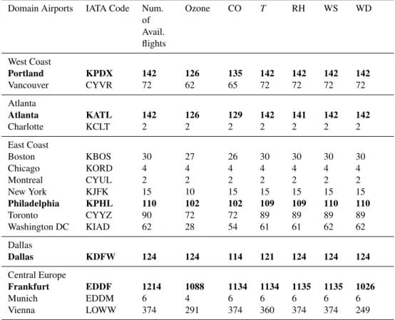
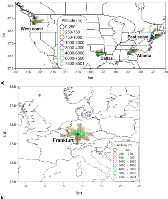
MOZAIC data were gathered during take-off and landing phases, with larger occurrences of early-to-mid-afternoon (corresponding to landings in NA) and mid-to-late afternoon (corresponding to take-offs in NA) local time flights, approx-imately 70 % of which occurred during spring and summer. Table 1 gives the list of airports within each simulation do-main and the number of MOZAIC flights associated with each airport during 2006. To simplify the analysis, the air-port with the largest number of flights is selected and used for the analysis. In total, five airports (four in NA and one in EU) are identified for analysis in this study. The Portland and Philadelphia airports are selected to represent the west and east coasts of NA, respectively, while the Dallas and At-lanta airports represent the two other areas of NA. Frankfurt (with over 1200 hourly flights) had the best yearly coverage and represents the central EU area. The locations of the air-ports and flight areas are shown in Fig. 1.
In addition to the MOZAIC measurements, ozonesonde data were extracted from the World Meteorological Orga-nization (WMO) World Ozone and Ultraviolet Radiation Data Centre in Toronto (Canada) and made available to the AQMEII community. These measurements report vertical profiles of ozone partial pressure at several vertical pressure levels. Further details on these data are given in Schere et al. (2012).
2.1 Pairing models and observational data
The groups participating in AQMEII were requested to de-liver their model results for the species, time, location, and altitude for which observational data were available. The model data corresponding to the three-dimensional grid en-closing the MOZAIC trajectories at the aforementioned 13 altitudes were subsequently delivered to European Commis-sion’s Joint Research Centre in Ispra (Italy) by each mod-elling group, with a common horizontal grid resolution for the whole period of 2006 with one-hour time resolution. Hosting the data is the ENSEMBLE system (Galmarini et al., 2004, 2012), a web-interfaced data hub allowing model and observed data to be harmonized and paired in time and space to facilitate the model evaluation. Once a specific air-port, date, and flight are selected, the ENSEMBLE system automatically extracts the model data from the domain vol-ume and couples them with the MOZAIC profiles in space and time. Since measurements and model results are stored in ENSEMBLE at the same heights, the trajectory analysis module in ENSEMBLE works by looping through the mea-surement points along each three-dimensional trajectory.
3 Participating models
The participating research groups and modelling systems used are reported in Table 2. In total, four to five (depending on the variable) groups delivered data to compare against the MOZAIC profiles for NA, whereas data from eight to nine groups were available for EU.
The emissions and chemical BCs used by the various AQMEII groups are summarised in Table 2. AQMEII pro-vided a set of reference time-varying gridded emissions (referred to as the “standard” emissions) for each conti-nent. These inventories have been extensively discussed in other AQMEII publications (Pouliot et al., 2012; Solazzo et al., 2012a, b). Although the standard emissions were used by the vast majority of the participating AQMEII groups, there were still a number of degrees of freedom (e.g. fire emissions or biogenic emissions) which were chosen by each group independently. Model results generated with other emissions inventories were also submitted. AQMEII also provided a set of time-dependent chemical concen-trations at the lateral boundaries of the EU and NA do-mains, referred to as the “standard” BCs, extracted from the Global and regional Earth-system Monitoring using Satel-lite and in-situ data (GEMS) re-analysis product provided by the European Centre for Medium-range Weather Forecast (ECMWF) (Schere et al., 2012). These standard BCs were used by the majority of the modelling groups, although other BCs for ozone were also used, which were based on satel-lite measurements assimilated within the Integrated Forecast System (IFS). Models were driven by different meteorologi-cal simulations, which were described and evaluated in Vau-tard et al. (2012). Details on the model configurations are given in Table 2.
3.1 Participating models and settings
3.1.1 WRF-CMAQ
Table 1.Airport domains and number of hourly flights during 2006 for each variable. The airports selected for analyses are highlighted in bold.
Domain Airports IATA Code Num. of Avail. flights
Ozone CO T RH WS WD
West Coast
Portland KPDX 142 126 135 142 142 142 142
Vancouver CYVR 72 62 65 72 72 72 72
Atlanta
Atlanta KATL 142 126 129 142 141 142 142
Charlotte KCLT 2 2 2 2 2 2 2
East Coast
Boston KBOS 30 27 26 30 30 30 30
Chicago KORD 4 4 4 4 4 4 4
Montreal CYUL 2 2 2 2 2 2 2
New York KJFK 15 10 15 15 15 15 15
Philadelphia KPHL 110 102 102 109 109 110 110
Toronto CYYZ 90 72 72 89 89 89 89 Washington DC KIAD 62 28 54 61 61 62 62
Dallas
Dallas KDFW 124 124 114 121 124 124 124
Central Europe
Frankfurt EDDF 1214 1088 1134 1134 1135 1135 1026
Munich EDDM 6 4 6 6 6 6 6
Vienna LOWW 374 291 374 360 374 374 249
3.1.2 ECMWF-SILAM
The SILAM (Sofiev et al., 2010) model uses a transport algo-rithm based on the non-diffusive Eulerian advection scheme of Galperin (1999, 2000) and the adaptive vertical diffusion algorithm of Sofiev (2002). The use of sub-grid variables in these schemes allows the model to be used with thick verti-cal layers. A detailed description of SILAM can be found in Sofiev et al. (2008). SILAM includes a meteorological pre-processor for diagnosing the basic features of the PBL and the free troposphere (e.g. diffusivities) from the meteo-rological fields provided by meteometeo-rological models (Sofiev et al., 2010). Only horizontal wind components are taken from the meteorological input, with the vertical component computed from the continuity equation. SILAM is a terrain-following height coordinate models, and for the AQMEII simulations the model consisted of nine layers up to approx-imately 10 km.
3.1.3 MM5-DEHM
The Danish Eulerian Hemispheric Model (DEHM) (Chris-tensen, 1997; Frohn et al., 2002; Brandt et al., 2012) is a 3-D long-range atmospheric chemistry-transport model with a horizontal domain covering the Northern Hemisphere with
150 km horizontal grid spacing. For AQMEII, the model in-cludes two two-way nested domains, one covering EU and one covering NA, and both with 50 km horizontal grid spac-ing. The vertical grid is defined using theσ-coordinate sys-tem, with 29 vertical layers extending up to 100 hPa. The hizontal advection is solved numerically using the higher or-der accurate space or-derivatives scheme, applied in combina-tion with a Forester filter (Forester, 1977). The vertical ad-vection, as well as the dispersion sub-models, is solved using a finite elements scheme for the spatial discretisation. For the temporal integration of the dispersion, the method is applied and the temporal integration of the three-dimensional advec-tion is carried out using a Taylor series expansion to third or-der. The three-dimensional wind fields are derived from the MM5 model, corrected in DEHM to ensure mass conserva-tion. DEHM also includes a module for diagnostically calcu-lating the vertical wind. For ozone, the initial and BCs (both lateral and top) are based on ozonesonde measurements, in-terpolated to global monthly three-dimensional values with a grid spacing of 4◦×5◦(Logan, 1999). A thorough description of DEHM and model set-up for AQMEII is given in Brandt et al. (2012).
a)
b)
Fig. 1.Flight trajectories by height for the selected airports in(a)North America and(b)Europe.
3.1.4 MM5-CHIMERE
The CHIMERE model (Bessagnet et al., 2004) applied over EU uses a 0.25◦(∼25 km) horizontal grid spacing and nine vertical layers expressed in a hybridσ-pressure coordinate system between surface and 500 hPa. The first near-surface layer height was 20 m. All meteorological fields are interpo-lated from the driver meteorology (MM5), with the vertical velocity recalculated to preserve mass balance. Turbulence in the PBL is represented using a diffusivity coefficient follow-ing the parameterization of Troen and Mahrt (1986) with-out the counter-gradient term. The second-order Van Leer scheme (Van Leer, 1979) is used for the horizontal trans-port, and horizontal diffusion is neglected. Top BCs are
ob-tained from the GEMS re-analysis at 3 h interval and inter-polated in three dimensions. The depth of the PBL is taken directly from MM5. Full model documentation is available at http://euler.lmd.polytechnique.fr/chimere
3.1.5 ECMWF-LOTOS-EUROS
Table 2.Participating models and features.
Met AQ model Resolution
(km)
Vertical (bottom-top)
Emission BC
North America
GEM AURAMS 15×15 28
(14 in the first 2 km)
Standardb Climatology
MM5 DEHM 50×50 29
(100 hPa)
Global emission database/ EMEPd
Estimated from hemispheric domain
WRF CMAQ 12×12 34
(25 m to 50 hPa)
Standard Standard
WRF CAM× 12 23
from 30 m
Standard Standard
Cosmo-CLM (CCLM)
CMAQ 24×24 30
(60 m to 100 hPa)
Standarda Standard
Europe
MM5 DEHM 50×50 29
(100 hPa)
Global emission database/EMEPd
Estimated from hemispheric domain
ECMWF SILAM 24 9
(10 km)
Standard Standard
MM5 CHIMERE 25 9
(20 m to 500 hPa)
Standard Standard,
MEGAN
ECMWF
LOTOS-EUROS
25 4 Standarda Standard
WRF CMAQ 18 34
(20 m to 50 hPa)
Standarda Standard
MM5 CAM× 15 23
(30 m to 12 km)
Standard Standard
WRF WRF-Chem1,2 22.5 35
(16 m to 50 hPa)
Supplied by WRF/Chem (constant background values)
Standard
Cosmo-CLM (CCLM)
CMAQ 24×24 30
(36 m to 100 hPa)
Standarda Standard
MM5 Polyphemus 24 9
(up to 1200 m)
Standarda,c Standard
aStandard anthropogenic emission and biogenic emission derived from meteorology (temperature and solar radiation) and land use distribution
implemented in the meteorological driver (Guenther et al., 1994; Simpson et al., 1995).bStandard anthropogenic inventory but independent emissions
processing, exclusion of wildfires, and different version of BEIS (v3.09) usedcEmissions include biomass burning, biogenic organic compounds of
SOA:α-pinene, limonene, sesquiterpene, and hydrophilic isoprene.
dGlobal: IPCC RCP 3-PD Lamarque et al. (2010); Bond et al. (2007); Smith et al. (2001); ships: Corbett and Fischbeck (1997); GEIA natural
emissions (Graedel et al., 1993); wildfires as in Schultz et al. (2008). Europe: EMEP (Vestreng and Støren, 2000)
of tracers is implemented in all three dimensions following Walcek (2000), where vertical mass fluxes are derived from the mass balance. Vertical mixing is primarily determined by the growth of the second model layer following the rise of the PBL during the day, which leads to mixing of con-centrations from the residual layer to the lower layer. Ad-ditional vertical mixing is implemented following standard K-diffusion (Louis, 1979). In the horizontal direction, no ex-plicit diffusivity was added, apart from the numerical diffu-sion implied by the advection on a discrete grid.
3.1.6 MM5-Polyphemus
The Polyphemus AQ modelling platform is used with the Polair3D Eulerian chemistry transport model (Sartelet et al., 2012). Over EU, the horizontal resolution is 0.25◦(∼25 km). Polyphemus used terrain-following height coordinates with nine vertical layers ranging from 20 m to 9 km for the AQMEII simulation. The reactive-transport equations are solved using operator splitting (sequence: advection, diffu-sion, chemistry and aerosol). The advection scheme is a di-rect space–time third-order scheme with a Koren flux limiter.
Diffusion and chemistry are solved with a second-order Rosenbrock method. The vertical eddy-diffusion coefficient is parameterized following Louis (1979), except in the un-stable convective PBL where the coefficients are calculated using the parameterization of Troen and Mahrt (1986). The horizontal diffusion coefficient is constant and equal to 10 000 m2s−1. In the AQMEII simulation, meteorologi-cal fields are interpolated from MM5, except for the eddy-diffusion coefficient and the vertical velocity, which are de-rived from the continuity equation.
3.1.7 GEM-AURAMS
The AURAMS model (Gong et al., 2006; Smyth et al., 2009) applied for AQMEII on the NA domain uses a secant polar-stereographic map projection true at 60◦N, with 45 km hori-zontal grid spacing. In the vertical, 29 layers are used with a terrain-following modified Gal-Chen vertical coordinate and relatively thin layers near the surface (the first five layers were located at 0, 14, 55, 120, and 196 m) increasing mono-tonically in thickness to a model top at approximately 22 km. Horizontal and vertical advection are both calculated using a semi-Lagrangian advection scheme (e.g. Pudykiewicz et al., 1997) with wind components provided by the GEM me-teorological model (Cˆot´e et al., 1998a, b; Mailhot et al., 2006). The vertical diffusion operator is solved using an im-plicit first-order Laasonen scheme, where the vertical eddy-diffusion coefficient is parameterized in GEM using a turbu-lence kinetic energy scheme (Benoit et al., 1989; B´elair et al., 1999). Horizontal diffusion is neglected. Model output is only saved for the first 20 layers, so vertical profiles are only available for the AURAMS model up to 5 km.
3.1.8 WRF-WRF/Chem
The only model with atmospheric chemistry coupled online with the meteorology applied within this study is the commu-nity WRF/Chem mode (Grell et al., 2005). The two instances of WRF/Chem applied for EU are the same in all aspects except that only one (referred to as WRF/Chem1) includes feedback of the direct and indirect aerosol radiative effects to meteorology. The other simulation that does not include the radiative feedback effects is referred to as WRF/Chem2. Both simulations are set up with a horizontal grid spac-ing of 22.5 km, 36 vertical layers, and identical physics and chemistry options as described by Forkel et al. (2012). Gas-phase/aerosol chemistry and non-hydrostatic physics within WRF/Chem are tightly coupled, with fifth-order horizontal, third-order vertical, and a third-order Runge–Kutta time inte-gration scheme (Skamarock et al., 2008). YSU PBL physics (Hong et al., 2006) are used for vertical mixing within the PBL. Boundary conditions for all species are derived from the default WRF/Chem configuration, which are designed to be representative of clean, mid-latitude Pacific Ocean condi-tions. In spite of major differences in simulated solar
radi-ation for cloudy conditions, only small differences between the two model versions were found, since simulatedT, mix-ing ratio, and wind are nudged to the drivmix-ing global analysis above the PBL for the simulations discussed here (Forkel et al., 2012).
3.1.9 Cosmo-CLM-CMAQ
At the Helmholtz-Zentrum Geesthacht (HZG) Institute, the CMAQ model is set up using 24 km horizontal grid spac-ing and 30 vertical layers for both continents. Eleven of the 30 layers are below 1000 m, with the lowest layer top at ap-proximately 36 m. Version 4.6 of the CMAQ (Matthias et al., 2010; Aulinger et al., 2011) model was used for the EU do-main, while version 4.7.1 of the model was used for NA (the same version as the other CMAQ participants). Horizontal and vertical advection schemes in CMAQ use a modifica-tion of the piecewise parabolic method (PPM; Colella and Woodward, 1984). At each grid cell, a vertical velocity com-ponent is derived from the horizontal advection that satisfies the continuity equation using the density from driving me-teorological model. In CMAQ 4.7.1, this scheme is further modified by adjusting the vertical velocities by the ratio of upwind fluxes to PPM-calculated fluxes. Vertical diffusion is based on the asymmetric convective model (ACM; Pleim and Chang, 1992). In both CMAQ 4.6 and 4.7.1, version 2 of the ACM (ACM2; Pleim, 2007, 2007a) is implemented. The minimum value for the eddy diffusivity depends on the land use of the individual grid cells and varies between 0.5 m2s−1 in grid cells with no urban areas and 2 m2s−1in grid cells that contain only urban area. Zero flux BCs are used at the horizontal borders and at the top of the domain.
3.1.10 WRF/MM5-CAMx
hybrid centred/upstream (space) scheme and vertical diffu-sion solved using K-theory.
4 Model performance in the troposphere
4.1 Mean vertical profiles
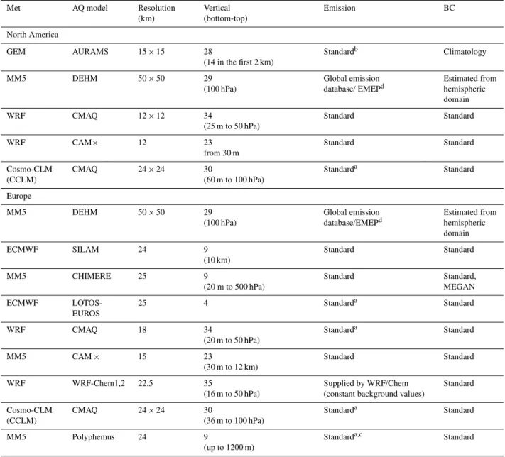
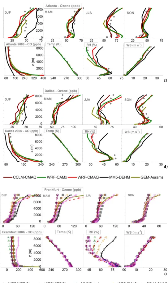
Figure 2 presents the comparison of modelled versus ob-served seasonally averaged mean profiles of ozone and an-nually averaged mean profiles of CO,T, RH and WS. Obser-vations are the grey symbols. While interpreting the results, it should be kept in mind that a source of model underes-timation may derive from the incommensurability of com-paring point measurements over airports to grid cell model values (Elguindi et al., 2010).
All models show similar mean profiles of wind above the PBL andT from the ground to higher level and in agreement with the observed profiles, most likely due to the nudging techniques applied to these fields. The MM5-DEHM is the only model with a positive bias for WS, which increases with altitude at all sites, possibly due to the grid spacing, which is two to three times coarser than the other models. Relative hu-midity profiles have the lowest bias within the first approx-imately 2 km, but significantly diverge above that height at all sites. It should be noted that in regions where the water vapour mixing ratio is very low (e.g. in the diverging zone), small differences inT can give rise to significant differences in RH. The RH peaks at 1000 m at all airports, although with different magnitudes. The peak is generally well captured by the models at all airports, with the exception of Dallas, where the bias at 1000 m ranges between 7 and 15 %.
The observed annual mean profiles of CO peak at ground level and diminish monotonically with altitude. The rate of decay is faster in the first 1.5–2.5 km (dependant on the airport) due to enhanced mixing near the surface, and is smoother aloft. This feature is common to all sites. The value of the observed CO peak ranges between a minimum of 166 ppb at Dallas and a maximum of 250 ppb at Frankfurt, with the remaining airports all in the range of approximately 200 ppb. Since CO is a directly emitted pollutant, its concen-tration is primarily determined by local emissions and BCs for CO. The modelled profiles of CO are significantly biased, typically with the largest bias near the ground, with few ex-ceptions. While the DEHM model is biased low throughout the altitudinal range at all sites, the other models tend to have high biases near the ground, the exception being the CCLM-CMAQ model, which performs the best in general, possibly due to a more effective vertical mixing scheme employed by the CCLM driver compared to the WRF driver for the other CMAQ simulations.
Mean profiles of observed CO show a steep decrease in mixing ratio in the first 2 km, with an average gradi-ent ranging between approximately−24 ppb km (Dallas and Philadelphia) and−37 ppb km (Atlanta), while Frankfurt is an outlier at−57 ppb km. Between 2 and 8 km, the rate of de-crease in CO mixing ratio is considerably less, with a gradi-ent of approximately 5–6 ppb km−1at all airports. Averaged profiles of modelled CO show that ground-level mixing ra-tios can differ by up to a factor of 2, although differences are smaller above the PBL, but still significant, as discussed in detail with the aid of Taylor diagram in Sect. 4.2.4 (the large range of the horizontal axis in Fig. 2 has the effect of cluster-ing the observed and modelled profiles at any given altitude, thus deceptively reducing the bias). A possible reason for the difference might be related to the horizontal grid spacing of the AQ model (e.g. Brunner et al., 2003). As shown in Ta-ble 2, the DEHM model, which has the coarsest horizontal grid resolution, simulated the lowest mixing ratios, whereas the CAMx and CMAQ models, with much smaller horizon-tal grid spacing, simulated the highest mixing ratios. Another possible reason could be related to the influence of the chem-ical BCs to CO and ozone. At the NA airports that are closer to the boundaries (i.e. Portland and Philadelphia), the mod-els that used GEMS BCs (i.e. CMAQ and CAMx) simulated CO mixing ratios that are closer in magnitude to each other than the DEHM and AURAMS models, which are driven by different BCs (model sensitivity to BCs is further discussed in Sect. 6).
The seasonally averaged ozone has the lowest mixing ra-tios in winter (all airports) and the typical maximum in spring and summer. The mean ozone mixing ratio increases with al-titude in the first 1000 m, as near-ground depletion by depo-sition and titration reduce the ozone availability (e.g. Cheva-lier et al., 2007). The effect of surface processes on ozone is also evident by the strong gradient in the first 2 km of the tro-posphere, ranging on average between 10 and 20 ppb km−1 at all sites. Modelled ozone mixing ratio in winter is typ-ically biased low at all locations, with the exception of the DEHM model (both NA and EU). The CCLM-CMAQ, MM5-CAMx, and SILAM for EU are all biased high above approximately 6 km throughout the year, likely due to inad-equate representation of the tropopause in the model, which results in too much mixing between the high stratospheric ozone mixing ratios in the BCs and the troposphere in the model. Ozone within the PBL is generally overestimated in the summer (NA only), while in the autumn the simulated mixing ratios are closer to the observed values, especially for Frankfurt. Layered ozone structures are most notable in summer months in the lowest levels close to the surface as result of the photochemistry and thermal mixing. At Port-land, by contrast, the observed ozone in June–August peaks at 3 km and is underestimated by all models. A relative min-imum of RH at the same height (annual average), which cor-responds to the plateau values (∼45 %) of RH above 3 km, might indicate a downward intrusion of ozone from the upper
a)
b)
Fig. 2.Seasonally averaged mean profiles of ozone (top rows) and annually averaged mean profiles of CO, temperature, relative humidity (RH) and wind speed (WS) (bottom rows) (year 2006) for(a)Portland,(b)Philadelphia,(c)Atlanta,(d)Dallas, and(e)Frankfurt. The grey symbols are the observations.
troposphere (Tulet et al., 2002). The lack of seasonal varia-tion of ozone for WRF/Chem in the upper air is due to the use of constant background values of ozone as BCs.
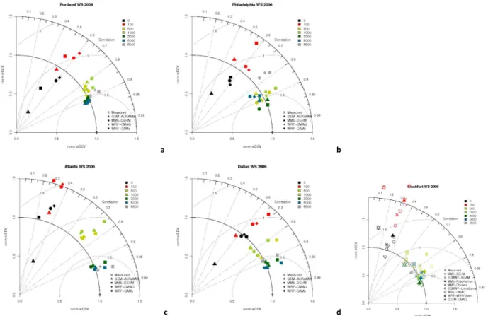
4.2 Operational statistics and variability
In this section, operational statistics are presented with the aid of Taylor diagrams (Taylor, 2001), which simultaneously show error, standard deviation and Pearson correlation co-efficient (PCC). In a Taylor diagram, the observed field is represented by a point at a distance from the origin along the abscissa that is equal to the variance. All other points on the plot area represent values for the simulated fields and are po-sitioned such that the variance of the modelled fields is the radial distance from the origin, the correlation coefficient of the two fields is the cosine of the azimuthal angle (desired value: 1), and the RMSE is the distance to the observed point
(desired value: 0). In practical terms, the closer a model point is to an observed point, the better the model performance.
c)
d)
36
e)
Fig. 2.Continued.
the airport. This aspect has an influence on the spread of the data. Coefficients of variation (CoVs), defined as the ratio between the standard deviation and the average of the an-nual distribution at any height, have been calculated in order to assess the model’s capability of reproducing the observed variability. For synthesis, CoVs are shown for Frankfurt only (Fig. 7), but are discussed for all airports.
Performance forT is considered to be satisfactory for all models, at all domains for at least the first 5 km (PCC in ex-cess of 0.90 and fractional bias≤1 %). For this reason, anal-ysis forT is not shown.
4.2.1 Wind speed
For all the airports, all models show significant errors in the modelled WS, and poor correlation with the observed val-ues in the first 100 m. Although the sign of the bias can-not be deduced from a Taylor diagram, further analysis (can-not shown) indicates that the models are biased high. Smaller er-rors (still positive bias) are also observed at 500 and 1000 m. Poor correlation and moderate to high error within the PBL are common to all models at all sites, thus indicating that the meteorological models are not reproducing WS in the PBL precisely, which is arguably the most important region of the atmosphere in relation to AQ processes. This result supports the findings by Vautard et al. (2012) for the ground-based measurements. The poor model performance in the first 100 m at all sites is also confirmed by the analysis of the CoV, with modelled values well below the observations.
A feature emerging is the clustering of performance based on altitude rather than on modelling system. For heights be-low the PBL, all models show the same deficiencies, indicat-ing that incorrect simulation of WS near the surface is a com-mon problem. There may be several reasons for this. First, near-surface winds are sensitive to several driving factors other than the synoptic circulation, such as land cover and surface energy exchange processes, which have been found to exhibit large model-to-model variability in global and re-gional models (e.g. see de Noblet-Ducoudr´e et al., 2012; Stegehuis et al., 2012). Second, unlike upper-air winds which are measured by rawinsondes and are incorporated in reanal-ysis products, surface winds are not used for producing re-analyses. Therefore, even with a strong nudging of the wind field to the reanalyses, a lower model skill is expected for sur-face winds as compared to upper-air winds. This is demon-strated by the improvement of model performance above 500 m. For all models at all sites, and more markedly at Port-land and Philadelphia, PCC, error and variability improve constantly with height. In general, the best performance by all models is observed forz≥3 km, with PCC>0.8 at all NA sites, with the exception of the WRF/Chem model (PCC∼0.65 atz=3 km), and at Frankfurt.
4.2.2 Wind direction
Although of pivotal importance for the transport of the pol-luted air masses, evaluation of the modelled WD is often overlooked. In this section we summarise the results of eval-uating the AQ models of Table 2 using observed WD data from ground to 8.5 km. To simplify the analysis we have binned the frequency counts of the occurrences of WD angle using a 20◦interval. Results are discussed in terms of nor-malised bias (modelled minus observed count, and divided by the observed count). In general, we find that the bias in the PBL for the Frankfurt airport is smaller and decreases faster with height than the NA airports. For the NA airports, in general there is a large bias within the PBL, which is most pronounced on the west coast (Portland).
For the Portland airport, WRF-CMAQ and GEM show similar biases from 0 to 500 m: positive for north-west and negative for south-east (∼100 %). The other models are bi-ased low in the eastern sector. Fromz=500 to 1000 m, the bias increases and all models show a clear tendency to over-estimate the occurrences of both westerly and easterly winds. Above the 1000 m height, the bias decreases and the mod-els better reproduce the frequency distribution of observed WD. On the east coast of NA (Philadelphia airport), iso-lated cases of large bias are present at the 500 m and 4 km heights, where the two WRF models are biased high in the north and south sectors, respectively. For the inland airports of Atlanta and Dallas, some occurrences of very large bias are observed. For the Atlanta airport, all models are biased high in the west and north-west directions (50 %) in the first 250 m. From 500 to 1000 m, the models are biased high (50 to 100 %) in the north-eastern and south-western directions. For the Dallas airport, the east-west positive bias (∼20 %) present for all of the models in the first 250 m turns clock-wise at 500 m, directed in the north-west direction. GEM and WRF-CAMx models also acquire a south-western bias component (about 70 %) at 1000 m. The bias progressively decreases above 2 km. At the Frankfurt airport, the models share similar bias patterns, at the ground, with a tendency to underestimate occurrences of northerly winds (all mod-els) and overestimate the westerly components (with differ-ent magnitude by all models).
37
a b
c d
e
Fig. 3.Taylor diagrams for wind speed at(a)Portland,(b)Philadelphia,(c)Atlanta,(d)Dallas and(e)Frankfurt. Height by colours, model by symbols.
4.2.3 Relative humidity
In contrast to WS, modelled values of RH exhibit a smaller increase in variability with height and vary more by site than WS (Fig. 4). The variability is underestimated by all mod-els, as shown by the normalised standard deviation of Fig. 4, most predominantly below unity at all airports, with the ex-ception of Portland where the variability in the first 1000 m is close to the observed variability. The best model perfor-mance for variability occurs between 500 and 1000 m, and then deteriorates with height. As stated earlier, this could be due to very small water vapour mixing ratio values aloft, which makes RH computation less reliable at higher alti-tudes. The analysis of the CoV reveals that the models tend to underestimate the observed variability in the free tropo-sphere, especially for z >6 km. Model performance is in general grouped by height, although with a few exceptions (such as the WRF/Chem at Frankfurt, Fig. 4e). The mini-mum model errors and maximini-mum PCC occur for altitudes in the range of 1 to 3 km, although with some exceptions (most notably Atlanta) and not consistently for all models. For ex-ample, the Taylor diagram for Frankfurt (Fig. 4e) reveals a large scatter of data independent of height and model, with the same model performing well in some instances
(LOTOS-EUROS at 3 km) but very poorly in others (the same model is off-scale at the surface). Further investigation is needed to determine whether the modelled variation of RH is not ill-treated, or in other words whether the modelling systems are getting the “right answer for the right reason”, which is one of the main objectives of the diagnostic model evaluation component defined in Dennis et al. (2010).
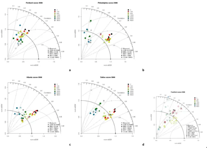
4.2.4 CO
Profiles of modelled CO show PCC values typically be-low 0.6 at all heights and airports, with a limited number of exceptions (e.g. WRF-CMAQ at Frankfurt, whose PCC above 3 km exceeds 0.7) (Fig. 5a). All of the models have difficulty reproducing the temporal variability of CO mixing ratios, possibly due to the influence of local sources close to the airport, whose temporal variation is not captured by the models due to too coarse grid spacing. Analysis of the CoV demonstrates that the variability is largely overestimated in the PBL at all NA airports (up to a factor of two at Dallas, Atlanta, and Philadelphia). CoV estimates improve slightly with height above the PBL, with the best agreement in the range of 2 to 4 km. This may be due to a stronger dependence on the large-scale transport from the BCs combined with the
39
a b
c d
e
Fig. 4.Taylor diagrams for relative humidity at(a)Portland,(b)Philadelphia,(c)Atlanta,(d)Dallas and(e)Frankfurt. Height by colours, model by symbols.
nudging of winds at these altitudes, while in the lower tro-posphere CO mixing ratios are the result of a more complex mix between transport and emission.
The analysis for CO was not separated by season, but as there are more measurements available in summer than in winter, a bias to summer months is expected in the Taylor di-agrams of Fig. 5a. CO concentrations are typically lower in the spring and summer than in winter at all altitudes with a minimum in July and maximum in February to April (Gilge et al., 2010; Elguindi et al., 2010). As a result, the annual mean deviation of the modelled to the observed profiles in Fig. 2 and the error in Fig. 5a are primarily associated with lower CO mixing ratios. Because model performance for CO is similar across all models, this may indicate problems with the inputs that were shared among the models. In par-ticular, the fact that at the ground the majority of models overestimate observed mixing ratios suggests that emissions from certain source categories, such as mobile sources or biomass burning, are overestimated. Another reason could be the emission profiles used. If CO is primarily emitted in the lowest layer, mixing ratios at the surface might be overesti-mated. This hypothesis could be explored further by compar-ing the vertical profiles of other more long-lived species, such as aerosols. However, it is beyond the scope of this study to
conclusively determine the reasons for the poor model per-formance near the surface.
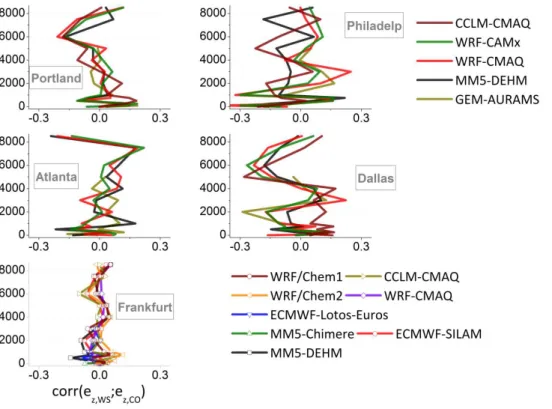
It is important to consider that biased meteorological drivers might have a bigger impact on long-lived species such as CO. Any error in the input wind field (speed and direc-tion) can accumulate over time, possibly exacerbating errors introduced by imperfect emission inventories. To test this hy-pothesis for CO, we calculated the correlation between the error in the modelled CO mixing ratio and the error in the WS at each given altitude and airport. Letcorr(fz,s1;gz,s2) be the operator returning the PCC of any two fieldsf andg
at heightzfor the speciess1ands2. Thencorr(ez,W S;ez,CO)
41 a
b
c
d e
Fig. 5a.Taylor diagrams for CO at(a)Portland,(b)Philadelphia,(c)Atlanta,(d)Dallas and(e)Frankfurt. Height by colours, model by symbols.
model/airport/height combinations. Nonetheless, this analy-sis demonstrates that an association exists in certain cases, which deserve further investigations. We also note that in-stances of anti-correlation (negative PCC) are also numer-ous. In these cases, a decrease in WS error corresponds to an increase in CO error and vice versa, but it is difficult to determine whether they are associated with vertical intrusion or should just be treated as uncorrelated. Finally, WS and CO errors at Frankfurt do not show any association and can be considered independent.
4.2.5 Ozone
Due to its adverse effects on human health, climate, and ecosystems, surface ozone is among the most extensively studied atmospheric trace gases. Solazzo et al. (2012a) have shown that overall the AQ modelling systems participating in AQMEII perform satisfactorily in reproducing ozone mix-ing ratios at ground level (showmix-ing better skill in NA than in EU). For most models and airports, the yearly averaged ozone scores of Fig. 6 indicate better performance near the
ground (z≤1000 m) than aloft. At Portland the scores un-der and above the PBL are overall comparable, and at Frank-furt several models have scores higher for altitude between 500 and 1000 m (PCC in excess of 0.7) than forz <500 m. The 1000 m height tends to mark a transition from the PBL regime, characterised by well-mixed dynamics and active photochemistry, to a tropospheric regime characterised by a more marked model-to-model variability. Similar conclu-sions were drawn by Chevalier et al. (2007).
No clear factor emerges for grouping the ozone skill scores in Fig. 6. The two simulations using CMAQ over NA (driven by WRF and CCLM) do not produce similar scores at any of the airports, although they share the same BCs and emis-sions. By contrast, CMAQ and CAMx, the two AQ models driven by WRF, have rather similar results, indicating that the meteorological driver may have a substantial weight in determining the skill for ozone (in particular PBL dynam-ics). However, this latter hypothesis is not confirmed by the Taylor plots for Frankfurt (WRF/Chem and CMAQ are both driven by WRF) though, as the scores are primarily grouped
43
Fig. 5b.Profiles of correlation between the WS and CO errors for the airports of Portland, Philadelphia (first row), Atlanta, Dallas (middle row) and Frankfurt (lower panel).
by AQ modelling system, with the two simulations of CMAQ producing similar scores.
The standard deviation and the CoV are generally overes-timated within the PBL and underesoveres-timated aloft, although with several exceptions depending on the site, height, and model used, especially at the Atlanta, Dallas, and Frankfurt airports where the variability score at high altitudes is com-parable to that in the PBL. WRF/Chem at Frankfurt shows the lowest variability at all heights, and close to zero for
z≥3 km, possibly because at these heights the simulated val-ues are already influenced to some extent by the WRF/Chem BCs (constant values), which are too low, particularly in the spring and summer, at and above that height (see Fig. 2). The DEHM model underestimates the CoV at all NA airports, possibly due to the use of RCP emissions and different set of BCs (see Table 2).
The variability and errors above 3 km and up to 8.5 km re-veal some model deficiencies. The mean seasonal profiles in Fig. 2 indicate that the models tend to underestimate ozone between 3 and 6 km, but they overestimate ozone mixing ra-tios above that height (see Frankfurt for example), though not systematically for all locations and all seasons. This could be due to an underestimation of the exchange between the upper troposphere and the lower stratosphere and/or diffu-sive model errors related to coarse vertical gridding. By con-trast, for the case of global-scale chemistry models, Brunner et al. (2003) reported a tendency of models to overestimate
ozone mixing ratios over NA between 5.5 and 8 km through-out the year (based on the period 1995–1998). However, while those results were averaged over the entire NA tinent, here we are comparing regional-scale models at con-siderably smaller scales, and the different behaviour could simply be attributed to the different grid sizing as well as the different time period.
5 Altitudinal correlations
In this section we investigate the degree of association be-tween the error at the ground and the error aloft (0<z≤ 8.5 km), measured by the PCC for each of the variables. With the terminology introduced in Sect. 4.2.4, the association is expressed ascorr(e0,s, ez,s), wheresis the variable under
44
a b
c d
e Figure 6 Taylor diagrams for ozone at a) Portland; b) Ph
Fig. 6.Taylor diagrams for ozone at(a) Portland,(b) Philadelphia,(c) Atlanta,(d) Dallas and(e)Frankfurt. Height by colours, model by symbols.
contributed to the large-scale circulation, we would expect that under- or over-estimation is observed simultaneously at different altitudes, and therefore correlated.
Figure 8 reports how the fractional difference (FD) at the ground is correlated with the FD aloft for all investigated air-ports. FD is defined as
FD= Mod−Obs
0.5(Mod+Obs), (1)
where Mod and Obs areN-length vectors denoting the mod-elled and the observed field value, respectively. HereN is the number of hourly flights available for the period being analysed (reported in Table 1). The correlations are calcu-lated between theN-length FD vector at the ground and the
N-length FD vector at other levels.
The profiles of FD correlations in Fig. 8 demonstrate that for the investigated fields (with some exceptions for CO as discussed below) positive correlations are limited to the PBL, and biases within the PBL are poorly correlated with those of the free troposphere at all airports. The gradient of the correlation profiles drops sharply with height for both WS
and RH. For these latter fields in particular, we observe the strongest vertical gradient as well as the most homogeneous behaviour among the different models, suggesting that the proper simulation of WS and RH in the PBL is principally determined by near-surface processes (the only exception is WRF/WRF-Chem at Frankfurt).
Correlation of FD profiles for CO exhibits a less homo-geneous behaviour. PCC varies aloft between 0.1–0.2 and 0.4–0.6, this latter value primarily associated with the MM5-DEHM modelling system, for which the hypothesis of large-scale error might explain the correlation between bias at the ground and aloft (note that DEHM results reflect the strong vertical mixing shown by the mean vertical profiles of Fig. 2). Correlation of FD profiles for ozone is more homogeneous than CO among the different models, supporting the propo-sition that the vertical ozone profile is the result of an inter-play between an ozone reservoir in the upper troposphere and ground-level mixing ratios (Zhang and Rao, 1999; Godow-itch et al., 2011. Overall, errors produced in the PBL for ozone remain contained within the PBL (all models show similar patterns) and are weakly connected with those above,
46 Figure 7. Modelled (vertical axis) versus observed (horizontal axis) coefficients of variation for
Fig. 7.Modelled (vertical axis) versus observed (horizontal axis) coefficients of variation for Frankfurt (year 2006) for (clockwise from top-left) ozone, CO, WS, and RH. The straight line is the perfect agreement. Height by colours, model by symbols.
although for Frankfurt this pattern is less pronounced. Above the PBL, and especially for the two CMAQ simulations at Portland and WRF/Chem at Frankfurt, the FD correlation profiles are more varied, typically low for CAMx (close to zero between 3 and 4 km at all airports) and scattered be-tween PCC values of 0 to 0.3 for the other models.
Although the altitudinal correlation analysis is very infor-mative about how far the errors at the ground propagate in the vertical, it cannot be considered exhaustive as it does not provide detailed insight into the modelling systems’ ability to represent specific processes. Instead, it reveals the need for a more quantitative evaluation of vertical mixing. This could be accomplished by comparing the modelled PBL height with measurements; however, these data were not collected within AQMEII.
6 Altitudinal error: the case of ozone
6.1 Aggregate seasonal error
The seasonal error associated with the model’s capability of estimating ozone mixing ratios in the vertical is investigated for all airports and models. The error is expressed as frac-tional absolute difference (FAD):
FAD= |Mod−Obs|
0.5(Mod+Obs) (2)
47
Fig. 8.Correlation coefficient between the fractional difference (FD) at any height and the FD at the ground (z=0) for ozone, CO, RH, and WS (columns) and for the airports of Portland, Philadelphia, Atlanta, Dallas, and Frankfurt (rows) (year 2006). The first line of the legend refers to the NA models, while the other two lines to Frankfurt.
Furthermore, the error of the WRF-CMAQ model at the ground at Philadelphia in winter is larger than the other in-stance of CMAQ driven by CCLM, likely due to a higher titration effect. Figure 2 also shows that WRF-CMAQ ex-hibits the highest CO mixing ratio, suggesting that differ-ences between the two CMAQ simulations may be due to the different vertical diffusion scheme used. Moreover, the dis-tribution of FAD from the CCLM-CMAQ model (negligible at ground and larger above 500 m) at Portland in winter and at Philadelphia and Dallas in summer suggests that CCLM-CMAQ is able to capture the surface layer equilibrium be-tween NOx and ozone better than the other models. It is also worth noting that the performance of CCLM-CMAQ aloft is comparable with those of the other models, indicating that surface-level processes are not strongly influenced by ozone
aloft. Finally, the large error at 8.5 km at Frankfurt is due to model top boundary being close to that height, as for example the SILAM model.
Overall the diversity of modelling errors both in the PBL (particularly in summer) and in the free troposphere (partic-ularly in winter) indicates a large range of differences in the AQ models, particularly at Frankfurt in both seasons. These differences relate to turbulence, transport, and photochem-istry in the PBL (the emissions are largely shared), and to grid spacing, top and lateral boundaries, and the advection schemes used in the free troposphere.
48
Fig. 9.Cumulative fractional absolute difference (FAD) of modelled ozone for the months of December, January, and February 2006.
Figure 10.Cumulative Fractional Absolute Difference (FAD) of modelled ozone for the months of June, Fig. 10.Cumulative fractional absolute difference (FAD) of modelled ozone for the months of June, July, and August 2006.
6.2 Bias due to boundary conditions
In this section we expand the model evaluation by provid-ing comparison between the lateral BCs for ozone and the vertical profiles of ozone measured on-board MOZAIC air-craft. We show the analysis for NA only, as the proximity of the airports to the edges of the modelled domain allows test-ing the influence of the BCs more effectively. Details about
the preparation of the standard BCs for AQMEII are given in Schere et al. (2012).
For the airports of Vancouver and Portland (west coast) and Philadelphia (east coast), we analyse the following hourly vertical profiles averaged over the months of January and August:
50 Figure 11. Positions where BCs data are provided for GEMS and DEHM (position for AURAMS is the
Fig. 11.Positions where BC data are provided for GEMS and DEHM (position for AURAMS is the same as for GEMS). For the east coast of NA, the locations of two ozonesondes used in the analysis are also shown. The shaded areas indicate the extension of the domain around the airport
51 Monthly averaged vertical profiles of ozone for Vancouver, January 2006: BCs providers
Fig. 12.Monthly averaged vertical profiles of ozone for Vancouver, January 2006: BC providers (thick lines), AQ model outputs (thin lines), MOZAIC (filled squares). The horizontal lines by the mea-surements are the standard deviations (symmetric about the mean point and only the left portion is shown).
– monthly ozone BCs adopted by the AQ models;
– monthly profiles of modelled ozone mixing ratio over the selected airports;
– monthly MOZAIC measurements of ozone at the se-lected airports and the observed standard deviation;
– ozonesonde data collected at rural locations falling within the MOZAIC domain for Philadelphia for the month of August 2006.
Results of the comparison are shown in Figs. 12 to 16. The GEMS BCs were adopted by the WRF-CMAQ,
52
Figure 13 Normalised modelled vs. BCs bias with respect to MOZAIC for the month of January 2006 for the Fig. 13.Normalised modelled vs. BC bias with respect to MOZAIC for the month of January 2006 for the Portland airport. The two CMAQ instances and CAMx use the same BCs. The continuous lines are derived from the linear regression fit, with the squared cor-relation coefficients reported on the top right corner (colour coded). In parentheses are the squared coefficients obtained by correlating the bias excluding the data in the first 250 m (i.e. by including data from 500 m to 8.5 km).
CCLM-CMAQ, and CAMx models (Table 2); the AURAMS group used its own BCs, while ozone BCs for DEHM were extracted from climatology and satellite measurements and applied to the model’s outer domain, which encompasses the entire Northern Hemisphere. The concentration profiles at the DEHM’s inner domains (one centred in NA and one in EU), which reflect the dynamics of the hemispheric domain, are taken here for comparison (the cells where the profiles were extracted are shown in Fig. 11).
During winter, the absence of strong photochemical activ-ity amplifies the influence of BCs. Forz >2 km, the ozone monthly profiles for both US coasts overlap to a large extent
53 Figure 14. Monthly averaged vertical profiles of ozone for Portland, August 2006. The BC for the
Fig. 14. Monthly averaged vertical profiles of ozone for Port-land, August 2006. The BC for the AURAMS model (thick orange line) was provided at Vancouver.
54 Figure 15 Monthly averaged vertical profiles of ozone for Philadelphia, January 2006.
Fig. 15.Monthly averaged vertical profiles of ozone for Philadel-phia, January 2006.
the corresponding boundary profiles (Figs. 13 and 15). The only exception is for DEHM, which shows a significant de-parture with altitude from the boundary profile, and, conse-quently, the bias with respect to the observed MOZAIC pro-files also reflects the error of the BCs for this model. For January at Vancouver and Philadelphia, the modelled profiles have sharper gradients within the PBL than aloft due to titra-tion, but the modelled ozone mixing ratios clearly show the influence of BCs acting as an offset to surface mixing ratios, confirming that during winter the mean bias in ground-level mixing ratios is mostly driven by the large-scale background mixing ratios. This is further demonstrated by the corre-lation analysis in Fig. 13, where we show the normalised bias of the BCs and modelled ozone mixing ratios with re-spect to MOZAIC measurements. The regression analysis
55 Figure 16 Monthly averaged vertical profiles of ozone for Philadelphia, August 2006. Monthly averaged
Fig. 16.Monthly averaged vertical profiles of ozone for Philadel-phia, August 2006. Monthly averaged ozonesonde profiles from two nearby rural locations (see Fig. 11) are also reported.
demonstrates the large degree of association between the bias of two fields (especially for AURAMS and WRF-CMAQ, with PCC of 0.86 and 0.75 respectively). When including only the bias from levels above 500 m in the analysis, the PCC values are even larger for all models, except for AU-RAMS, which has fewer data available as the top of the model domain extends to only 5 km. This confirms the find-ings of Schere et al. (2012) regarding the penetration of the bias induced by the BCs for ozone far into the interior of the model simulation domain, which they found to be espe-cially true for winter months and for rural areas away from major emission sources. Systematic underestimation of tro-pospheric ozone by the global modelling systems that were used to derive the BCs for the AQMEII modelling caused the regional-scale models to frequently underestimate near-surface ozone mixing ratios in NA.
Different behaviour is observed in summer. At Port-land (Fig. 14) all models underestimate the observed mixing ratio above 2 km, with the GEMS BCs also underestimat-ing the MOZAIC measurements. Below 1000 m, all models overestimate the observed mixing ratios by approximately 20–25 ppb, possibly due to an overestimation of vertical mix-ing in the PBL. It should be further noted that the distance between Portland and the coast is approximately 100 km, and therefore the grid cell over the airport does not include any ocean area (model grid spacings are well below 100 km); thus there should not be any gradient between deposition over ocean and over land leading to overestimation of modelled ozone. At 1000 m height, the bias between the models and MOZAIC is smallest before turning positive at 2 km, with the modelled profiles unable to replicate the sharp gradient ob-served in the MOZAIC data. Such a gradient is possibly due to titration of NOX surface emissions together with surface
the airport is expected to increase the ozone gradient in the lowest levels due to fast titration by NO. This effect is ex-pected to vanish aloft (Chevalier et al., 2007). Differences in the aloft BCs are also seen in the aloft modelled values, and in turn in the ground-level mixing ratios. This is not the case for DEHM, where once again the vertical mixing appears to play the dominant role. Overall, the BCs do not appear to be the primary driver for the bias on the west NA coast during summer.
At the Philadelphia airport, the models tend to slightly un-derestimate (5 to 10 ppb) ozone mixing ratios for August 2006 (Fig. 16) above 4 km, while there is an overestima-tion of 6 to 20 ppb below 1000 m. The models driven by the BCs provided by GEMS and, to a lesser extent, AURAMS replicate very well the observed profile between 1.5 and 3 km, while DEHM is biased high. GEMS profiles are biased low above 4 km, but are in agreement with MOZAIC obser-vations from the ground up to 1.5 km. The models driven by the GEMS BCs (the two instances of CMAQ and CAMx) show some differences within the first 3 km, though they cluster around the corresponding boundary value in the up-per levels. The bias at these altitudes is possibly influenced by the GEMS BCs. The spread among the models is likely driven by photochemistry, the effect of which is stronger in Philadelphia than in Portland, being that the east coast has higher NOx emissions than the western areas (e.g. see Appel et al., 2012). Ground-level ozone mixing ratios sim-ulated from models driven by GEMS range between 45 and 65 ppb, consistent with the notion that local production en-hances summer ozone mixing ratios in polluted areas more than the large-scale background mixing ratios. This result is also shared by DEHM, which exhibits the highest surface mixing ratios, although it had the lowest boundary mixing ratio values. Profiles of ozone mixing ratios measured by ozonesondes for August were available from two rural sites (Fig. 11) within the Philadelphia domain, and are reported in Fig. 16. Measurements at the site STN487 (∼370 km north-east of the airport, close to the coast) were collected daily for August at 18:00 GMT, while 12 h measurements from the STN420 (∼160 km south-west of the airport) were col-lected between 04:00 GMT and 20:00 GMT. Profiles from STN420 are similar to those of the MOZAIC in the first 1000 m but diverge from the modelled mixing ratios more than the MOZAIC above 1000 m. The profiles from this ru-ral ozonesonde station therefore suggest that the GEMS BCs may be biased low at this site (also found by Schere et al., 2012). Ozone mixing ratios from station STN487 also sup-port this inference, as they are also close to the MOZAIC values in the upper levels. Finally, ozonesonde profiles from both sites confirm that the modelled ozone mixing ratios are biased high in the first 1000 m.
7 Summary and conclusions
This study has been conducted in the framework of the AQMEII activity and presents an evaluation of regional-scale AQ models in the troposphere supported by measurements gathered in the MOZAIC campaign. Fifteen regional-scale modelling groups from EU and NA have produced three-dimensional data of ozone, CO, WS, WD, RH and T with hourly resolution for the full year of 2006 at selected areas around major airports in EU and NA. These data have been paired with MOZAIC vertical profiles by the ENSEMBLE platform.
The scope of this study is the operational evaluation of the AQ modelling systems, i.e. the comparison of model results to observed data, supported by error metrics and variance statistics to gauge model performance in an overall sense. Results are thus based on the operational statistics obtained by comparing modelled against measured profiles. Several cases exhibiting significant differences between observations and model predictions have been identified as potential sub-jects of more in-depth diagnostic analysis to be undertaken in future.
From the study of the annual average mean vertical pro-files of WS, we conclude the following:
– Above the PBL, there is little model-to-model vari-ability at all airports, with all models showing similar mean profiles, most likely due to observational nudg-ing. MM5-DEHM is the only model with a positive bias for WS, which increases with altitude at all sites, and is likely due to the coarser grid spacing used.
– For winds within the PBL (which are not nudged), all models (at all airports) show significant errors (predom-inantly as a positive bias) and poor correlation with the observed WS values in the first 100 m, and generally up to 500 m, with smaller errors between 500 and 1000 m. In addition, most models underestimated the variabil-ity within the first 100 m at all airports, indicating that the meteorological models are still weak in reproduc-ing WS in the PBL. Factors that could contribute to the poor performance include sensitivity of the near-surface winds to influences other than the synoptic circulation (e.g. land cover), and processes driving the exchange of energy at surface for which global and regional mod-els are known to largely differ from one another. For all models and at all airports, PCC, error and variability improve consistently with altitude. In general, the best performance by all models was observed forz≥3 km with a PCC>0.8 at all NA airports and, with the ex-ception of the WRF/Chem model, at Frankfurt as well. We also investigated the model-to-model bias in predict-ing the frequency of WD counts when the whole wind rose is binned into 20◦intervals, at all heights. We find the follow-ing: