c
Uma Publicação da Sociedade Brasileira de Matemática Aplicada e Computacional.
Stability Boundary Characterization
of Nonlinear Autonomous Dynamical Systems
in the Presence of Saddle-Node Equilibrium Points
1
F.M. AMARAL2
, Departamento de Ensino, Instituto Federal de Educação, Ciência e Tecnologia Bahia, Campus Eunápolis, 45.822-000 Eunápolis, BA, Brasil.
L.F.C. ALBERTO3
, Departamento de Engenharia Elétrica, Escola de Enge-nharia Elétrica de São Carlos, Universidade de São Paulo, 13.566-590 São Carlos, SP, Brasil.
Abstract. A dynamical characterization of the stability boundary for a fairly large class of nonlinear autonomous dynamical systems is developed in this paper. This characterization generalizes the existing results by allowing the existence of saddle-node equilibrium points on the stability boundary. The stability boundary of an asymptotically stable equilibrium point is shown to consist of the stable manifolds of the hyperbolic equilibrium points on the stability boundary and the stable, stable center and center manifolds of the saddle-node equilibrium points on the stability boundary.
Keywords. Stability Region, Stability Boundary, Saddle-Node Equilibrium Point.
1.
Introduction
Asymptotically stable equilibrium points of many practical nonlinear dynamical systems are not globally stable. As a consequence, the determination of stability regions (region of attraction or basin of attraction) of asymptotically stable equi-librium points is a fundamental problem in nonlinear system theory [10] with great importance in several applications [19, 17, 4]. The exact stability region is of diffi-cult determination and, over the last thirty years, a great number of methods were proposed for estimating the stability region of attractors of nonlinear dynamical systems [16].
Some recent methods, such as those developed in [8] and [4], explore a topological characterization of the stability boundary (the boundary of the stability region) to obtain good estimates of the stability region. Therefore, developing characte-rizations of stability boundaries of nonlinear dynamical systems is of fundamental importance for developing efficient tools for stability region estimation.
1
The authors would like to thank FAPESP (research project 2010/00574-9) and CNPq (Con-selho Nacional de Desenvolvimento Científico e Tecnológico) for the financial support.
2
3
Under some reasonable assumptions, the stability boundary of an asymptotically stable equilibrium point was characterized in terms of the stable manifolds of a set of unstable equilibria (and/or closed orbits) lying on this boundary [6]. These existing characterizations of stability boundaries were proved under the key assumption that all the equilibrium points on the stability boundary are hyperbolic. A first generalization of this characterization appeared in [2] by considering the existence of a particular type of non-hyperbolic equilibrium point, the so called type-zero saddle-node equilibrium point, on the stability boundary. In this paper, a further generalization of this characterization of the stability boundary is developed by allowing the presence of any type of saddle-node equilibrium point on the stability boundary. The characterization of the stability boundary in the presence of saddle-node equilibrium points is of fundamental importance for studying stability region bifurcations [3].
In this paper, a complete characterization of the stability boundary of nonlinear dynamical systems possessing saddle-node equilibrium points on it is presented. It is shown that the stability boundary consists of the stable manifolds of the hyper-bolic equilibrium points on the stability boundary and the stable, stable center and center manifolds of the saddle-node equilibrium points on the stability boundary. Necessary and sufficient conditions for a saddle-node equilibrium point lying on the stability boundary are also developed.
2.
Preliminaries
In this section, some classical concepts of the theory of dynamical systems are reviewed. In particular, an overview of the main features of the dynamic behavior of a system in the neighborhood of a specific type of non-hyperbolic equilibrium point, the saddle-node equilibrium point, is presented. More details on the content explored in this section can be found in [11, 21, 18].
Consider the nonlinear autonomous dynamical system
˙
x = f(x) (2.1)
where x∈ Rn. One assumes thatf : Rn → Rn is a vector field of class Cr with
r≥2. The solution of (2.1) starting atxat timet= 0is denoted byϕ(t, x). The map t → ϕ(t, x) defines in Rn a curve passing through xat t = 0 that is called
trajectoryororbitof (2.1) throughx. IfM is a set of initial conditions, thenϕ(t, M)
denotes the set {ϕ(t, x), x ∈M} =Sx∈Mϕ(t, x). A setS ∈ Rn is said to be an
invariant set of (2.1) if every trajectory of (2.1) starting inS remains inS for allt.
2.1.
Hyperbolic equilibrium points
A point x∗ ∈
Rn is an equilibrium point of (2.1) if f(x∗) = 0. An equilibrium point x∗ is said to be hyperbolic if none of the eigenvalues of the Jacobian matrix
Df(x∗)off(x), calculated at the equilibrium pointx∗, has real part equal to zero. Moreover, a hyperbolic equilibrium point x∗ is of type-k if the Jacobian matrix
Let x∗ be a hyperbolic equilibrium point of the nonlinear dynamical system (2.1). Then there exists a neighborhood U of x∗ and local stable and unstable manifolds[13], Ws
loc(x∗) ={x∈U :ϕ(t, x)→x∗ as t→ ∞}andWlocu (x∗) ={x∈
U : ϕ(t, x) → x∗ as t → −∞} with the following properties: (i) they have the same dimensions as those of the eigenspaces Es and Eu of the linearized system
˙
z=Df(x∗)z, therefore the sum of the dimension ofWs loc(x
∗)and ofWu loc(x
∗)equals the dimension of the state space; (ii) they are tangent toEsandEu atx∗; and (iii) they are as smooth as functionf.
Thestable manifoldWs(x∗)and the unstable manifoldWu(x∗), which are in-variant sets, are obtained by letting the points in Ws
loc(x∗) to flow backwards in
time and the points inWu
loc(x∗)to flow forwards in time [22]:
Ws(x∗) =[
t≤0
ϕ(t, Ws loc(x
∗)) Wu(x∗) = [
t≥0
ϕ(t, Wu loc(x
∗)).
2.2.
Saddle-Node equilibrium points
In this section, a specific type of non-hyperbolic equilibrium point, namely saddle-node equilibrium point, is studied. In particular, the dynamical behavior in a neighborhood of the equilibrium is investigated, including the asymptotic behavior of solutions in the invariant local manifolds.
Definition 2.1. [21](Saddle-Node Equilibrium Point): A non-hyperbolic equi-librium pointp∈Rnof (2.1) is called a saddle-node equilibrium point if the following conditions are satisfied:
(i) Dxf(p) has a unique simple null eigenvalue and none of the other eigenvalues
have real part equal to zero.
(ii)w(D2
xf(p)(v, v))6= 0,
with v as the right eigenvector and w the left eigenvector associated with the null eigenvalue.
Saddle-node equilibrium points can be classified in types according to the num-ber of eigenvalues ofDxf(p)with positive real part.
Definition 2.2. (Saddle-Node Equilibrium Type): A saddle-node equilibrium point p of (2.1), is called a type-k saddle-node equilibrium point if Dxf(p) has k
eigenvalues with positive real part andn−k−1 with negative real part.
Ifpis a saddle-node equilibrium point of (2.1), then there exist invariant local manifoldsWs
loc(p),W cs loc(p),W
c loc(p),W
u
loc(p)andW cu
loc(p)of classC
r, tangent toEs,
Ec⊕Es,Ec,EuandEc⊕Euatp, respectively [13]. These manifolds are respectively
called stable, stable center, center, unstable and unstable center manifolds. The stable and unstable manifolds are unique, but the stable center, center and unstable center manifolds may not be.
Ifpis a saddle-node equilibrium point, then the following properties hold [21]:
(i) The (n−1)-dimensional local stable manifold Ws
loc(p) of p exists, is
unique, and if q∈Ws
loc(p)thenϕ(t, q)−→past−→+∞.
(ii) The unidimensional local center manifoldWc
loc(p)ofpcan be splitted in
two invariant submanifolds:
Wc
loc(p) =W c−
loc(p)∪W c+ loc(p)
where q ∈ Wc−
loc(p) impliesϕ(t, q) −→p as t −→ +∞ and q ∈Wc +
loc(p)
implies ϕ(t, q) −→ pas t −→ −∞. Moreover,Wc+
loc(p)is unique while
Wc−
loc(p)is not.
(2) pis a type-ksaddle-node equilibrium point of (2.1) with1≤k≤n−2:
(i) Thek-dimensional local unstable manifoldWu
loc(p)ofpexists, is unique,
and ifq∈Wu
loc(p)thenϕ(t, q)−→past−→ −∞.
(ii) The(n−k−1)-dimensional local stable manifoldWs
loc(p)ofpexists, is
unique, and if q∈Ws
loc(p)thenϕ(t, q)−→past−→+∞.
(iii) The(n−k)-dimensional local stable center manifoldWcs
loc(p)ofpcan be
splitted in two invariant submanifolds:
Wcs
loc(p) =W cs−
loc (p)∪W cs+ loc (p)
where q∈Wcs−
loc (p) impliesϕ(t, q)−→pas t−→+∞. The local stable
center manifold Ws
loc(p)is contained in Wcs −
loc (p), moreover,Wcs − loc (p)is
unique while Wcs+
loc (p)is not.
(iv) The(k+ 1)-dimensional local unstable center manifoldWcu
loc(p)ofpcan
be splitted in two invariant submanifolds:
Wcu
loc(p) =W cu−
loc (p)∪W cu+ loc (p)
whereq∈Wcu+
loc (p)impliesϕ(t, q)−→past−→ −∞. The local unstable
center manifoldWu
loc(p)is contained inW cu+
loc (p), moreover,W cu+ loc (p)is
unique while Wcu−
loc (p)is not.
(3) pis a type-(n−1)saddle-node equilibrium point of (2.1):
(i) The (n−1)-dimensional local unstable manifold Wu
loc(p) of pexists, is
unique, and if q∈Wu
loc(p)thenϕ(t, q)−→past−→ −∞.
(ii) The unidimensional local center manifoldWc
loc(p)ofpcan be splitted in
two invariant submanifolds:
Wc
loc(p) =W c−
loc(p)∪W c+ loc(p)
where q ∈ Wc−
loc(p) impliesϕ(t, q) −→p as t −→ +∞ and q ∈W c+ loc(p)
implies ϕ(t, q)−→ pas t −→ −∞. Moreover, Wc−
loc(p)is unique while
Wc+
Figure 1: ManifoldsWcs−
loc (p)andW cu+
loc (p)for a type-1 saddle-node equilibrium pointp
of system (2.1) inR3 .
Although the stable and unstable manifolds of a hyperbolic equilibrium point are defined by extending the local manifolds through the flow, this technique cannot be applied to general non-hyperbolic equilibrium points. However, in the particular case of a saddle-node equilibrium pointp, one still can define the global manifolds
Ws(p), Wu(p), Wc+
(p), Wc−
(p), Wcs−
(p) and Wcu+
(p) extending the local ma-nifoldsWs
loc(p),W u loc(p),W
c+ loc(p),W
c− loc(p),W
cs−
loc (p)andW cu+
loc (p)through the flow
as follows:
Ws(p) :=[
t≤0
ϕ(t, Wlocs (p)) W u
(p) :=[
t≥0
ϕ(t, Wlocu (p))
Wcs−
(p) := [
t≤0
ϕ(t, Wcs−
loc (p)) Wcu +
(p) :=[
t≥0
ϕ(t, Wcu+ loc (p))
Wc−
(p) := [
t≤0
ϕ(t, Wc−
loc(p) and Wc +
(p) :=[
t≥0
ϕ(t, Wc+ loc(p)).
This extension is justified by the aforementioned invariance and the asymp-totic behavior of the local manifolds Ws
loc(p), Wlocu (p), Wc +
loc(p), Wc −
loc(p), Wcs − loc (p)
and Wcu+
loc (p), see items (1), (2) and (3) above. Figure 1 illustrates the manifolds
Wcs−
loc (p)andWcu +
loc (p)for a type-1 saddle-node equilibrium pointp.
2.3.
Stability Region
Suppose xs is an asymptotically stable equilibrium point of (2.1). The stability
region (or region of attraction) ofxs is the set
A(xs) ={x∈
Rn : ϕ(t, x)→xs as t→ ∞},
of all initial conditions x∈ Rn whose trajectories converge to xs when t tends to
The stability region A(xs) is an open and invariant set. Its closure A(xs) is
invariant and thestability boundary ∂A(xs), the topological boundary ofA(xs), is
a closed and invariant set.
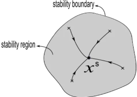
Figure 2: Stability region and stability boundary of an asymptotically stable equilibrium pointxs
.
3.
Hyperbolic Equilibrium Points on the Stability
Boundary
In this section, an overview of the existing body of theory about the stability bound-ary characterization of nonlinear dynamical systems is presented. The unstable equilibrium points that lie on the stability boundary∂A(xs)play an essential role
in the stability boundary characterization.
Let xs be a hyperbolic asymptotically stable equilibrium point of (2.1) and
consider the following assumptions:
(A1) All the equilibrium points on∂A(xs)are hyperbolic.
(A2) Every trajectory on∂A(xs)approaches an equilibrium point as t→+∞.
Assumption (A1) is a generic property of dynamical systems in the form of (2.1). In other words, it is satisfied for almost all dynamical systems in the form of (2.1) and, in practice, does not need to be verified. On the contrary, assumption (A2) is not a generic property of dynamical systems and needs to be checked. In spite of that, many nonlinear dynamical systems satisfy this property. In particular, the existence of an energy function is a sufficient condition to guarantee the satisfaction of (A2) [6].
Under assumptions(A1)and(A2),the next theorem provides a complete characterization of the stability boundary ∂A(xs). It asserts that the stability
boundary ∂A(xs)is the union of the stable manifolds of the unstable equilibrium
points on∂A(xs).
Theorem 3.1. (Stability boundary characterization)[6] Let xs be an
as-sumptions(A1) and(A2)are satisfied, then:
∂A(xs)⊆[ i
Ws(xi)
wherexi,i= 1,2, ...are the hyperbolic equilibrium points on the stability boundary
∂A(xs). If, in addition, Wu(xi)∩A(xs)6=∅,i= 1,2, ..., then
∂A(xs) =[ i
Ws(xi).
Theorem 3.1 provides a complete stability boundary characterization of system (2.1) under assumptions (A1) and (A2). Sufficient conditions to guarantee that
Wu(xi)∩A(xs) 6= ∅ when a hyperbolic equilibrium point xi ∈ ∂A(xs) are also
provided in [6].
4.
Saddle-Node Equilibrium Points on the Stability
Boundary
In the presence of non hyperbolic equilibrium points on the stability boundary, Theorem 3.1 is not valid. In this section, a generalization of the results of Theorem 3.1 about stability boundary characterization is developed. We study the stability boundary characterization when assumption(A1)is violated. In particular, a com-plete characterization of the stability boundary is developed when a particular type of non-hyperbolic equilibrium point, the so called saddle-node equilibrium point, lies on the the stability boundary∂A(xs).
Next theorem offers necessary and sufficient conditions to guarantee that a saddle-node equilibrium point lies on the stability boundary in terms of the pro-perties of its stable, unstable and center manifolds.
Theorem 4.1. (Saddle-Node Equilibrium Point on the Stability
Boun-dary): Letpbe a saddle-node equilibrium point of (2.1). Suppose also, the existence of an asymptotically stable equilibrium pointxs and letA(xs)be its stability region.
Then the following holds:
(i) Ifpis a type-0 saddle-node equilibrium point, then:
p∈∂A(xs)⇔(Wc+
(p)− {p})∩A(xs)6=∅
p∈∂A(xs)⇔(Ws(p)− {p})∩∂A(xs)6=∅.
(ii) Ifpis a type-k saddle-node equilibrium point, 1≤k≤n−2, then:
p∈∂A(xs)⇔(Wcu+
(p)− {p})∩A(xs)6=∅
(iii) Ifpis a type-(n−1) saddle-node equilibrium point, then:
p∈∂A(xs)⇔(Wcu+(p)− {p})∩A(xs)6=∅.
Proof. (i) The proof of item(i)can be found in [2].
(ii) (⇐=) Suppose first that (Wcu+(p)− {p})∩A(xs) 6= ∅. Then there exists
x ∈ Wcu+
(p)∩A(xs). Note that ϕ(t, x) −→ p as t −→ −∞. On the other
hand, set A(xs)is invariant, thusϕ(t, x)∈A(xs)for all t≤0. As a consequence,
p ∈ A(xs). Since p /∈ A(xs), we have that p ∈ (Rn −A(xs)). Therefore, p ∈
∂A(xs). Now if (Ws(p)− {p})∩∂A(xs) 6= ∅ then there exists at least a point
x∈ (Ws(p)− {p})∩∂A(xs). Moreover, ϕ(t, x) → pas t → ∞. Since ∂A(xs) is
closed and invariant, thenp∈∂A(xs).
(ii) (=⇒) Suppose thatp∈ ∂A(xs). Let Dcu be a neighborhood of pin Wcu(p),
whose boundary ∂Dcu is transversal to the vector field f on Wcu+, and define Dcu+ :=Dcu∩Wcu+(p). ConsiderLcu+
ǫ ={x∈Rn : d(x, ∂Dcu +
)< ǫ}for some
ǫ >0. As a consequence ofλ-lemma for non-hyperbolic equilibrium points [18], we can take a neighborhoodU ofpsuch that∪t≤0ϕ(t, Lcu
+
ǫ )⊃(U− {Wcs −
(p)}). Since
p∈∂A(xs), we have thatU∩A(xs)6=∅. On the other hand, asWcs−
(p)∩A(xs) =∅,
we can affirm that(U−{Wcs−
(p)})∩A(xs)6=∅. Thus, there exists a pointq∗∈Lcu+ ǫ
and a time t∗ such thatϕ(t∗, q∗)∈A(xs). SinceA(xs) is invariant, we have that
q∗∈A(xs). Sinceǫcan be chosen arbitrarily small, we can find a sequence of points
{q∗
i} withq∗i ∈A(x
s)for all i= 1,2, ... such thatd(q∗
i, ∂D cu+
)→0 as i−→+∞. By construction, this sequence is bounded, so has a convergent subsequence, that is, q∗
ij → q as ij → +∞. Thus, d(q
∗
ij, ∂D
cu+
) → d(q, ∂Dcu+
) as ij −→ +∞ and
consequentlyq∈∂Dcu+
⊂(Wcu+
(p)−{p}). Therefore(Wcu+
(p)−{p})∩A(xs)6=∅.
The proof thatp∈∂A(xs)⇔(Ws(p)−{p})∩∂A(xs)6=∅and of item(iii)is similar
to the above proof and will be omitted.
Letxs be an asymptotically stable equilibrium point of (2.1) and consider the
following assumption:
(A1′) All the equilibrium points on ∂A(xs) are either hyperbolic or saddle-node
equilibrium points.
Under assumptions(A1′)and(A2), next theorem offers a complete characteri-zation of the stability boundary of nonlinear autonomous dynamical systems in the presence of saddle-node equilibrium points on the stability boundary∂A(xs).
Theorem 4.2. (Stability Boundary Characterization): Let xs be an asymp-totically stable equilibrium point of (2.1) and A(xs) be its stability region. If
assumptions (A1′)and(A2) are satisfied, then
∂A(xs)⊆[ i
Ws(x i)
[
j
Ws(p j)
[
l
Wcs−
(zl)
[
m
Wc−
(qm)
wherexi are the hyperbolic equilibrium points,p
j the type-0saddle-node equilibrium
the type-(n−1) saddle-node equilibrium points on∂A(xs),i, j, l, m= 1,2, .... If, in
addition, Wc+(p
j)∩A(xs)6= ∅, for all j = 1,2, ... and the unstable manifolds of
all other equilibrium points on the stability boundary ∂A(xs)intersect the stability
regionA(xs), then:
∂A(xs) =[ i
Ws(x i)
[
j
Ws(p j)
[
l
Wcs−
(zl)
[
m
Wc−
(qm).
Proof. If q ∈ ∂A(xs), from assumptiom (A2), we can affirm that ϕ(t, q) −→ q∗ for some equilibrium point q∗ ∈ ∂A(xs). From assumptiom (A1′
), we can af-firm that q∗ is either a hyperbolic equilibrium point or a saddle-node equilibrium point, that is, q∗ = x
i or q∗ = pj or q∗ = zl or q∗ = qm for some i, j, l, m.
Since, the intersection Wc−
(pj)∩∂A(xs) is empty [2], we can affirm that q ∈
S
iW s(x
i)SjWs(pj)SlWcs −
(zl)SmWc −
(qm). Therefore, ∂A(xs) ⊆ SiWs(xi)
S
jW s(p
j)SlWcs −
(zl)SmWc −
(qm). In order to prove the other inclusion, we
ex-plore the facts thatWu(x
i)∩A(xs)6=∅for alli= 1,2, . . .,Wu(zl)∩A(xs)6=∅for all
l= 1,2, . . .,Wu(q
m)∩A(xs)6=∅for allm= 1,2, . . .andWc+(pj)∩A(xs)6=∅for all
j= 1,2, . . .. Ifzlis a typeksaddle-node equilibrium point, with1≤k≤n−2, on
∂A(xs), then, by assumption,Wu(z
l)∩A(xs)6=∅, then there isw∈Wu(zl)∩A(xs).
LetB(w, ǫ)be an open ball with an arbitrarily small radius ǫcentered at w. Ra-dius ǫ can be chosen arbitrarily small such that B(w, ǫ) ⊂ A(xs). Let q
1 be an arbitrary point ofWcs−
(zl)and consider a diskD of dimensionkthat is
transver-sal to Wcs−
(zl) at q1. As a consequence of λ-lemma for non-hyperbolic equilib-rium points [18], there exists an element z ∈ D and a time t∗ > 0 such that
ϕ(t∗, z)∈B(w, ǫ). SinceA(xs)is invariant, we have thatz∈A(xs). Sinceǫand the
diskD can be chosen arbitrarily small, then there exist points ofA(xs)arbitrarily
close toq1. Thereforeq1∈A(xs). SinceWcs
−
(zl)cannot contain points onA(xs),
q1∈∂A(xs). Exploring the fact that q1was arbitrarily taken inWcs
−
(zl), we can
affirm thatWcs−
(zl)⊂∂A(xs). Similarly, it can be shown thatWs(xi)⊂∂A(xs),
Ws(p
j)⊂∂A(xs)andWc −
(qm)⊂∂A(xs), consequently the theorem is proven.
Theorem 4.2 is more general than Theorem 3.1, since assumption(A1), used in the proof of Theorem 3.1, is relaxed. It also generalizes the results in [2] where only type-zero saddle-node equilibrium points were considered.
5.
Example
The system of differential equations (5.1) was derived from problems of stability in power systems analysis [9]:
˙
x = 1−2,84sen(x)−2sen(x−y) ˙
y = 1−3sen(y)−2sen(y−x) (5.1)
stable equilibrium point xs = (0.35; 0.34)and two type-1 saddle-node equilibrium
points on the stability boundary ∂A(xs), they are; q
1 = (1,42; 3,39) and q2 =
(2,12;−3,87). Moreover, eight unstable hyperbolic equilibrium points also belong to the stability boundary∂A(xs). The stability boundary∂A(0,35; 0,34)is formed,
according to Theorem 4.2, as the union of the manifoldsWc−
(q1),Wc
−
(q2)and the stable manifolds of the unstable hyperbolic equilibrium points that belong to the stability boundary, see Figure 3.
Figure 3: The gray area is the stability region of the asymptoticaly stable equilibrium point xs. The stability boundary ∂A(0,35; 0,34) is formed by the stable component of the center manifolds of the saddle-node equilibrium pointsq1 andq2 union with the stable manifolds of all the unstable hyperbolic equilibrium points that belong to the stability boundary.
6.
Conclusions
This paper developed the theory of stability region of nonlinear dynamical systems by generalizing the existing results on the characterization of the stability boundary of asymptotically stable equilibrium points. The generalization developed in this paper considers the existence of a particular type of non-hyperbolic equilibrium point on the stability boundary, the so called saddle-node equilibrium point. Necessary and sufficient conditions for a saddle-node equilibrium point lying on the stability boundary were presented. A complete characterization of the stability boundary when the system possesses saddle-node equilibrium points on the stability boundary was developed for a large class of nonlinear dynamical systems. This characterization is an important step to study the behavior of the stability boundary and stability region under parameter variation.
equilíbrio assintoticamente estável consiste das variedades estáveis dos pontos de equilíbrio hiperbólicos na fronteira da região de estabilidade e das variedades es-táveis, centro-estáveis e centrais dos pontos de equilíbrio sela-nó na fronteira da região de estabilidade.
Palavras-chave. Região de estabilidade, fronteira da região de estabilidade, ponto de equilíbrio sela-nó.
References
[1] L.F.C. Alberto, H.D. Chiang, Uniform approach for stability analysis of fast subsystem of two-time scale nonlinear systems, Int. J. Bifurcat Chaos Appl. Sci. Eng.,17(2007), 4195-4203.
[2] F.M. Amaral, L.F.C. Alberto, Stability Boundary Characterization of Nonlinear Autonomous Dynamical Systems in the Presence of a Type-Zero Saddle-Node Equilibrium Point, Tendências em Matemática Aplicada e Computacional, 11
(2010), 111–120.
[3] F.M. Amaral, L.F.C. Alberto, Stability region bifurcations of nonlinear au-tonomous dynamical systems: type-zero Saddle-node bifurcations,International Journal of Robust and Nonlinear Control,21, No. 6 (2011), 591-612.
[4] H.D. Chiang, F. Wu, P.P. Varaiya, Foundations of direct methods for power sys-tem transient stability analysis,Institute of Electrical and Electronics Engineers Trans. on Circuits and Systems,34, No. 2 (1987), 160-173.
[5] H.D. Chiang, F. Wu, P.P. Varaiya, Foundations of the potential energy boundary surface method for power transient stability analysis,Institute of Electrical and Electronics Engineers Trans. on Circuits and Systems,35, No. 6 (1988), 712-728.
[6] H.D. Chiang, M.W. Hirsch, F.F. Wu, Stability region of nonlinear autonomous dynamical systems, Institute of Electrical and Electronics Engineers Trans. on Automatic Control,33, No. 1 (1988), 16-27.
[7] H.D. Chiang, J.S. Thorp, Stability regions of nonlinear dynamical systems: a constructive methodology, Institute of Electrical and Electronics Engineers Transactions on Automatic Control,34, No. 12 (1989), 1229-1241.
[8] H.D. Chiang, L. Fekih-Ahmed, Quasi-stability regions of nonlinear dynamical systems: optimal estimations, Institute of Electrical and Electronics Engineers Trans. on Circuits and Systems,43 , No. 8 (1996), 636-643.
[9] H.D. Chiang, “Direct Methods For Stability Analysis of Electric Power Systems - Theoretical Foundation" , Bcu Methodologies, And Applications, John Wiley and Sons, 2010.
[11] J. Guckenheimer, P. Holmes, “Nonlinear Oscilations,Dynamical Systems and Bifurcations of Vector Fields”, Springer -Verlag, New York, 1983.
[12] V. Guillemin, A. Pollack, “Differential Topology”, Englewood Cliffs, NJ: Prentice-Hall, 1974.
[13] M.W. Hirsch, C.C. Pugh, M. Shub, Invariant manifolds, Bull. Amer. Math. Soc.,76, No. 5 (1970), 1015-1019.
[14] W. Hurewicz., H. Wallman, “Dimension Theory”, Princeton, NJ: Princeton University Press, 1948.
[15] P. Kokotovic, R. Marino, On vanishing stability regions in nonlinear systems with high-gain feedback,Institute of Electrical and Electronics Engineers Trans. Automat. Contr.,31, No. 10 (1986), 967-970.
[16] M. Loccufier, E. Noldus, A new trajectory reversing method for estimating stability regions of autonomous dynamic systems, Institute of Electrical and Electronics Engineers Nonlinear Dyn.,21(2000), 265-288.
[17] R.M. May, “Stability and Complexity in Model Ecosystems”, Princeton, NJ: Princeton University Press, 1973.
[18] J. Palis, On morse-smale dynamical systems,Topology, 8, 385-405.
[19] R.M. Peterman, A simple mechanism that causes collapsing stability regions in exploited salmonid populations,J. Fish. Res. Board Can.,34, 1977.
[20] S. Smale, Differentiable dynamical systems,Bull. Amer. Math. Soc.,73(1967)
747-817.
[21] J. Sotomayor, Generic bifurcations of dynamical systems. In Dynamical Systems, (1973), 549-560.