Wrappers Feature Selection in Alzheimer’s Biomarkers
Using kNN and SMOTE Oversampling
†Y.E. RODRIGUES1*, E. MANICA1, E.R. ZIMMER2, T.A. PASCOAL3,
S.S. MATHOTAARACHCHI3 and P. ROSA-NETO3
Received on December 20, 2015 / Accepted on February 7, 2017
— For the Alzheimer’s Disease Neuroimaging Initiative (ADNI)**
ABSTRACT.Biomarkers are characteristics that are objectively measured and evaluated as an indicator of normal biological processes, pathogenic processes or pharmacological responses to a therapeutic interven-tion. The combination of different biomarker modalities often allows an accurate diagnosis classificainterven-tion. In Alzheimer’s disease (AD), biomarkers are indispensable to identify cognitively normal individuals des-tined to develop dementia symptoms. However, using the combination of canonical AD biomarkers, studies have repeatedly shown poor classification rates to differentiate between AD, mild cognitive impairment and control individuals. Furthermore, the design of classifiers to access multiple biomarker combinations includes issues such as imbalance classes and missing data. Due to the number of biomarkers combina-tions wrappers are used to avoid multiple comparisons. Here, we compare the ability of three wrappers feature selection methods to obtain biomarker combinations which maximize classification rates. Also, as the criterion to the wrappers feature selection we use thek-nearest neighbor classifier with balance aids, random undersampling and SMOTE oversampling. Overall, our analyses showed how biomarkers combi-nations affect the classifier precision and how imbalance strategy improve it. We show that non-defining and non-cognitive biomarkers have less precision than cognitive measures when classifying AD. Our approach surpasses in average the support vector machine and the weightedk-nearest neighbor classifiers and reaches 94.34±3.91% of precision reproducing class definitions.
Keywords:k-nearest neighbor, SMOTE, feature selection, Alzheimer’s biomarkers, Alzheimer’s disease classification.
†Work presented at Congress of Applied and Computational Mathematics – CMAC SE 2015.
*Corresponding author: Yuri Elias Rodrigues – E-mail: [email protected]
1Instituto de Matem´atica e Estat´ıstica – IME, Universidade Federal do Rio Grande do Sul – UFRGS, 91509-900 Porto Alegre, RS, Brasil. E-mail: [email protected]
2Instituto do C´erebro do Rio Grande do Sul – InsCer, Pontif´ıcia Universidade Cat´olica do Rio Grande do Sul – PUCRS, 91410-000 Porto Alegre, RS, Brasil. E-mail: [email protected]
1 INTRODUCTION
Alzheimer’s disease (AD) is the most common cause of dementia worldwide, posing enormous economic and social costs for the society [1]. AD [2] is pathophysiologically characterized by the gradual brain deposition of amyloid plaques, neurofibrillary tangles, and eventual neuronal depletion [2]. The AD spectrum is composed by preclinical (CN), mild cognitive impairment (MCI) and AD dementia phases [2]. Preclinical AD individuals are those cognitively normal with amyloid plaques and tangles, individuals with MCI have cognitive symptoms without meet-ing clinical criteria for dementia, and AD dementia individuals present severely compromised cognitive faculties [3]. In recent years, a plethora of biomarkers has been developed in order to track AD progression, such as biomarkers for beta peptide 1-42 (Aβ1−42) and tau proteins
that indicate the presence of the hallmark pathological features of AD, amyloid plaques, and neurofibrillary tangles, respectively [1, 2].
It is a well-established fact that combined biomarkers provide higher classification rates than single biomarkers [4]. In this regard, neuropsychological tests associated with different bio-marker modalities have been used to classify AD [5]. These studies have combined positron emission tomography (PET), magnetic resonance imaging (MRI), functional magnetic resonance imaging (fMRI) as well as cerebrospinal fluid (CSF) and blood biomarkers to perform binary classifications of AD [1], e.g. healthy versus unhealthy individuals. Despite AD’s classification problem being an inherently multiclass binary classification multiclass driven by binary strategies are the rule [1]. This happens since some classifiers are naturally binary and must be adapted to be multiclass by means of one-versus-all and one-versus-one strategies, e.g. support vector machine (SVM) [6]. Thus, to solve ann-class problem using binary classifiers, n(n2−1) rules are required to build a multiclass classifier. As benefit, binary classifiers are well suited for the receiver oper-ator characteristic (ROC) analysis [7] which has been largely applied in AD comparative studies, biomarkers model selection and conversion diagnosis prediction.
methods when the distribution mechanisms are known. Alternatively, the methods are mainly based on the creation of synthetic data for minor classes or/and pruning data for major classes [11].
There is a need to identify biomarker combinations that maximize the classification and un-derstand how much they contribute to differentiate between AD classes [13, 1]. However, this goal faces multiple classifier’s comparisons when assessing biomarker combinations. In order to avoid the excessive number of comparisons, feature selection techniques are able to find a set of biomarkers that meet defined criteria [14]. For a given task (e.g. classification) exam-ples of criteria are: to identify the most cost-effective biomarkers, with higher precision and low false-positive, find a subspace of reduced dimensionality with the same or enhanced discriminant properties; extract/build relevant features from raw data [15].
Techniques of feature selection have been largely applied to AD-related problems, intending to provide a better understanding of biomarkers relationship [13] and achieve defined criteria of usefulness [14]. Interesting applications of feature selection techniques contributed to the under-standing of AD, like the construction of potential biomarkers for enhanced classification. For instance, Lopez-de-Ipi˜na et al. owing to determine preclinical biomarkers for AD apply fea-ture selection techniques on spontaneous speech to extract discriminant feafea-tures [16]. They also were able to correctly classify AD subjects using kNN and multilayer perceptron (MLP) classi-fiers obtaining accuracy of 87.30% and 90.90%, respectively to each classifier. Feature selection AD-related also is found in the gene microarray analysis [15] and neuroimaging both with high-dimensional feature spaces and its own big data challenges. These fields have been provoking adaptation of feature selection techniques to deal with high dimensionality (tens of thousands features) and small sample size in the case of microarray datasets [15]. In neuroimaging, the feature selection methods in 3D matrices are able to mitigate performances issues and improve the classification accuracy [17].
minority oversampling technique (SMOTE) and the random undersampling. All algorithms and plot codes are available on-linehttps://github.com/yurier/TEMA-R-CODES.
2 METHODS
2.1 Dataset
Data used in the preparation of this article were obtained from the ADNI database (adni.loni.usc.edu). The ADNI was launched in 2003 as a public-private partnership, led by Principal Investigator Michael W. Weiner, MD. The goal of ADNI has been to test whether serial MRI, PET, other biological markers, and clinical and neuropsychological assessment can be combined to measure the progression of MCI and early AD. For up-to-date information, see www.adni-info.org. Features in this work consist of two neuroimaging biomarkers (labels 1,2), four neuropsychological tests (labels 3,4,5,6) and two proteomic biomarkers (la-bels 7,8) [19], respectively: 2-[18F]fluoro-2-Deoxy-D-glucose (FDG) PET, florbetapir-fluorine-18 (florbetapir-fluorine-18F-AV-45) PET, clinical dementia rating sum of boxes (CDRSB), Alzheimer’s disease as-sessment scale-cognitive with 11 items (ADAS11), mini mental state examination (MMSE), Ray auditory verbal learning test percent forgetting (RAVLT), Aβ1−42CSF, phosphorylated tau
pro-tein (p-tau181) CSF. Table 1 depicts dataset demographics.
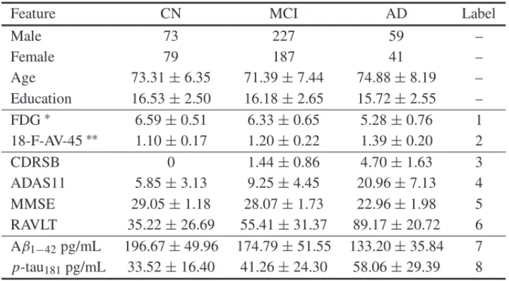
Table 1: Dataset demographics described by mean and standard deviation.
Feature CN MCI AD Label
Male 73 227 59 –
Female 79 187 41 –
Age 73.31±6.35 71.39±7.44 74.88±8.19 –
Education 16.53±2.50 16.18±2.65 15.72±2.55 –
FDG∗ 6.59±0.51 6.33±0.65 5.28±0.76 1
18-F-AV-45∗∗ 1.10±0.17 1.20±0.22 1.39±0.20 2
CDRSB 0 1.44±0.86 4.70±1.63 3
ADAS11 5.85±3.13 9.25±4.45 20.96±7.13 4
MMSE 29.05±1.18 28.07±1.73 22.96±1.98 5
RAVLT 35.22±26.69 55.41±31.37 89.17±20.72 6
Aβ1−42pg/mL 196.67±49.96 174.79±51.55 133.20±35.84 7
p-tau181pg/mL 33.52±16.40 41.26±24.30 58.06±29.39 8
Due to different probability in pathologies stages, clinical datasets are subject to imbalanced classes. Also, the data imbalance is a critical issue that generates an unfair separation between classes, when the imbalance is extreme [12] it will lead to decreased prediction rates for valida-tion stages. The present study evaluates two strategies to adjust the class imbalance by assum-ing any class posterior distribution. Since we are usassum-ing the kNN that is a distance based algo-rithm features were scaled by min-max normalization in all experiments [21] except for figures. Importantly, since features CDRSB and MMSE are employed to define the diagnosis or are similar to categorization protocol they will be used as contrast. The feature-wise comparison will be performed only for non-defining and non-cognitive features since it is well known that cognitive measures have more discriminative power [1]. Moreover, feature selection will be applied for non-defining features which include cognitive measures.
2.2 k-nearest neighbors (kNN) algorithm
Classifiers can be defined by discriminant functions [18], which are a set of functions to predict categorical dependent patterns. Here, we define a classifierCas a function that assigns a pattern x∈Rnto a class into the class spaceω∈:= {ω1, . . . , ωc},
C(x):Rn→.
Themaximum a posteriori(MAP) classifier uses a set of discriminant functions to assign the most probable class. Let{fωi(x)}
c
i=1be a set of discriminant functions, a classifierC is said to
be well-defined if, for all patterns, is possible to assign a class. Letω˜ be the calculated class, the MAP classifier is given by,
˜
w:=arg max
ω∈ fωi(x)=
C(x). (2.1)
The discriminant functions set is monotonous, since for a given x associated to a class ωj
we have that fωi(x) ≥ fωj(x)∀i = j. An example of a set of discriminant functions is the class conditional probability{p(x|ωi)}ci=1[18]. The classifiers taxonomy is based on how they
approximate its discriminant functions [6].Generative models parametrically approximate the posterior class probabilities,p(x|ωi), through the class conditional probability p(ωi|x)and the
class prior probability, p(ωi)(e.g. gaussian, gamma, etc). Alternatively, discriminative
mod-els directly approximate posterior class probabilities, p(ωi|x), without assuming a distribution
for it (e.g. kNN, MLP, etc). Aside from generative and discriminative models, there are the non-probabilistic models in which the discriminant functions are not required to be a distribution (e.g. SVM). Generally, the goal of discriminant functions is to divide the pattern space into decision regions{R1, . . . ,Rc}. Class densities are depicted in Figure 1 and the classification mapping
example is depicted in Figure 2. Also, Figure 2 shows a binary classification problem for feature combination labels 7 and 8 in which overlapped regions are subject to higher misclassification.
assuming Gaussian shapes the Bhattacharyya coefficient coincides with Mahalanobis measure. The Bhattacharyya coefficient [22] derived from Bhattacharyya distance ranges between 0 (distri-bution non-overlapped) and 1 (distri(distri-bution overlapped). Assuming normal distri(distri-butions between CN and AD distribution the Bhattacharyya coefficient is 0.6398824. Further this measure will be used to show how oversampling modifies the original distribution.
0 50 100 150
100 150 200 250 300
Aβ1−42 pg/mL
p-tau
181
pg/mL
0 50 100 150
100 150 200 250 300
Aβ1−42 pg/mL
p-tau
181
pg/mL
0 50 100 150
100 150 200 250 300
Aβ1−42 pg/mL
p-tau
181
pg/mL
level 0.00 0.05 0.10 0.15 0.20
class AD CN
Figure 1: On the left and middle, class distributions for CN and AD classes, respectively. On the right, AD and CN classes distribution overlapped in some regions.
0 50 100 150
100 150 200 250 300
Aβ1−42 pg/mL
p-tau
181
pg/mL
probability 0.00 0.25 0.50 0.75 1.00
class AD CN
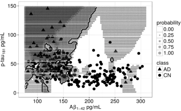
Figure 2: Decision boundaries created by the 3NN classifier.
The kNN is a non-parametric classifier that estimates the class posterior probability assuming that nearest patterns (here assumed to be vectors in a metric space) have similar properties (classes) [23]. This assumption was proved for infinite sample case as shown in [23]. There are preprocessing techniques, which depend on kNN, for instance: in data imbalance, complet-ing misscomplet-ing values, dimensionality reduction, and metric learncomplet-ing. Here we focus specifically on data imbalance challenge and a feasible solution; SMOTE algorithm.
The kNN classifier deals with multiclass problems straightforwardly by means of all-versus-all strategy. To achieve this, it uses a neighborhood defined byktraining instances nearest to a query instance to be classified. LetT = {(xi, ωi)}mi=1be a training set, with tuplesxi ∈Rnandωi ∈
a classω∗ ∈ . Using the MAP framework given in equation (2.1) the kNN classifier can be written as,
˜
ω∗=arg max
ω∈
xj∈N(x∗,k)
δ(ωj, ω), (2.2)
where N(x∗,k)is a neighborhood withktraining instances around x∗ for a given metric and
δ(., .)is the Kronecker delta function. Rewriting equation (2.2) we have,
˜
ω∗=arg max
⎧ ⎨
⎩
xj∈N(x∗,k)
δ(ωj, ω1), . . . ,
xj∈N(x∗,k)
δ(ωj, ωc)
⎫ ⎬
⎭
. (2.3)
The monotonicity of discriminant functions is applied to equation (2.3) and dividing it byk,
˜
ω∗=arg max
⎧ ⎨
⎩
xj∈N(x∗,k)
δ(ωj, ω1)
k , . . . ,
xj∈N(x∗,k)
δ(ωj, ωc)
k
⎫ ⎬
⎭
. (2.4)
Thus, each term in equation (2.4) is the posterior class probability,
p(ωi|x∗,k,T)=
xj∈N(x∗,k)
δ(wj, wi)
k , from i =1, . . . ,c. (2.5)
From equation (2.5) we have that the most probable class for the training instancex∗is given by,
˜
ω∗=arg max
ω∈p(ω|x∗,k,T). (2.6)
The parameterkthat adjusts thek-neighborhoodN(x∗,k)is searched empirically since there are no guidelines for its optimality. However, Bhattacharyya [24] proposes a bound to the optimalk, that isk<√m. In binary classification, one can restrain the range ofkby using only odd values in order to avoid ties in equation (2.1). The class posterior distribution,p(ωj|x), is an alternative
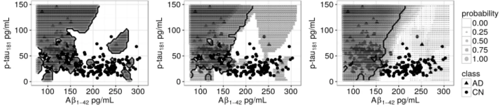
to the optimum Bayesian classification approach, which requires the complete knowledge of data generation underlying mechanisms. As showed by Cover & Hart [25], the error of the nearest neighbor is limited between the optimal error and twice the optimal error for the infinite sample case. This means that the more data available the closer the optimum error will be. This was supported by Stone on the existence of a universally consistent classifier [23]. Let’s show how the parameters affect the classifier properties. Figure 3 depicts the role of parameter k in the decision regions as well as the probability of class assignment described by the equation (2.6). Also, in Figure 3, note that there are only two probability values fork = 1 (1NN classifier). This happens since there are no misclassification errors or ties for training set in 1NN. A perfect score in training set would be an indicator of overfitting that generally leads to poor performance issues, that is, the classifier is unable to generalize the training results. Contrasting to 1NN, when parameterkis increased, more data is needed in order to evaluate the pattern assignment leading to more stratified probability values.
0 50 100 150
100 150 200 250 300
Aβ1−42 pg/mL
p-tau
181
pg/mL
0 50 100 150
100 150 200 250 300
Aβ1−42 pg/mL
p-tau
181
pg/mL
0 50 100 150
100 150 200 250 300
Aβ1−42 pg/mL
p-tau
181
pg/mL
probability 0.00 0.25 0.50 0.75 1.00
class AD CN
Figure 3: Left to right, the influence of parameterkin the decision boundaries, fork=1,k=5 andk=15, respectively.
training dataT andkto approximate the class posterior distribution. That is to say, data modifica-tion or removals imply in different classifiers sinceT is modified. By that, the biomarker combi-nations are validated using 10-fold CV and LOOCV in order to observe the variation between dif-ferent training data sizes. Although, variations using the same dataset also can occur due to ties in kNN. For instance, with 5NN some query pattern class could be evaluated as “AD+AD+CN+ CN+MCI”. The random tie-breaking is adopted in this work because is computationally more efficient than tie-breaking strategies described in [26]. Figure 4 shows the effect of random tie breaking in the decision regions for the three class problem proposed.
0 50 100 150
100 150 200 250 300
Aβ1−42 pg/mL
p-tau
181
pg/mL
0 50 100 150
100 150 200 250 300
Aβ1−42 pg/mL
p-tau
181
pg/mL
0 50 100 150
100 150 200 250 300
Aβ1−42 pg/mL
p-tau
181
pg/mL
probability 0.00 0.25 0.50 0.75 1.00
class AD CN MCI
Figure 4: Decision region for a three class problem solved with 5NN using the same number of samples for each class. From left to right, decision region of CN, MCI and AD, respectively.
One can observe in Figure 4, apart from noisy region created by the random tie breaking, the decision regions are complementary. Furthermore, unlike the binary case that requires only one class posterior probability to describe the classification mapping, the multiclass problem needs all the posterior probabilities to describe the classification mapping. For instance, binary mapping needs only to evaluate p(ω2|x) =1−p(ω1|x)and the decision border can be described with p(ω1|x) = p(ω2|x) = 0.5. In turn, the multiclass problems need all posteriors{p(ωi|x)}ci=1
high-dimensional spaces using a weighted schemeW(., .)as an argument of a kernel function
K(.). This is to adjust relative distances between patterns avoiding the sparsity [27]. Further-more, fractional metric modifications in kNN (or metric based classifiers) also can grant some level of reliability in high-dimensional feature spaces [28]. The wkNN can be written as,
˜
ω∗=arg max
ω∈
xj∈N(x∗,k)
δ(ωj, ω)K(W(x∗,xj)), (2.7)
where the weighted scheme [27] can be defined as follows,
W(x∗,xj)=
d(xk,x∗)−d(xj,x∗)
d(x1,x∗)−d(xk,d∗) if d(xk,x∗)=d(x1,x∗)
1 otherwise
2.3 SMOTE
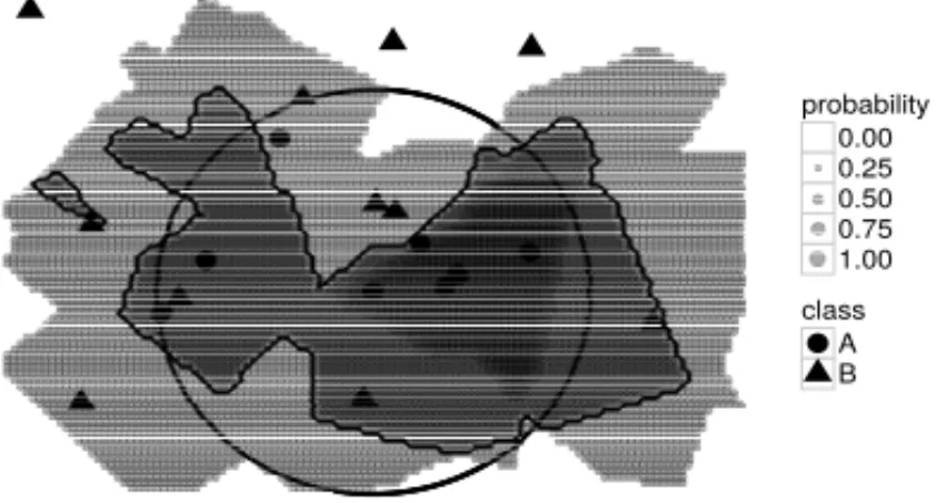
Data imbalance shows to be an adverse setup to achieve high classification rates. This happens due to the rare or less frequent instances of minor represented classes (e.g. bank fraud, cancer malignancy grading) [12]. When the minority class has few training patterns it turns out to be misrepresented leading to shrunken decision regions. For instance, in Figure 5 the minor class was generated inside the circle with uniform distribution with 8 samples while the major class follows the distributionN([2,2],4I)with 100 samples generated from it.
probability 0.00 0.25 0.50 0.75 1.00
class A B
Figure 5: Decision region for an imbalanced dataset. The irregular solid line is the decision border between class A and B.
effect of undersampling and oversampling techniques that are data-level methods since data is balanced disregarding the subsequent classifier.
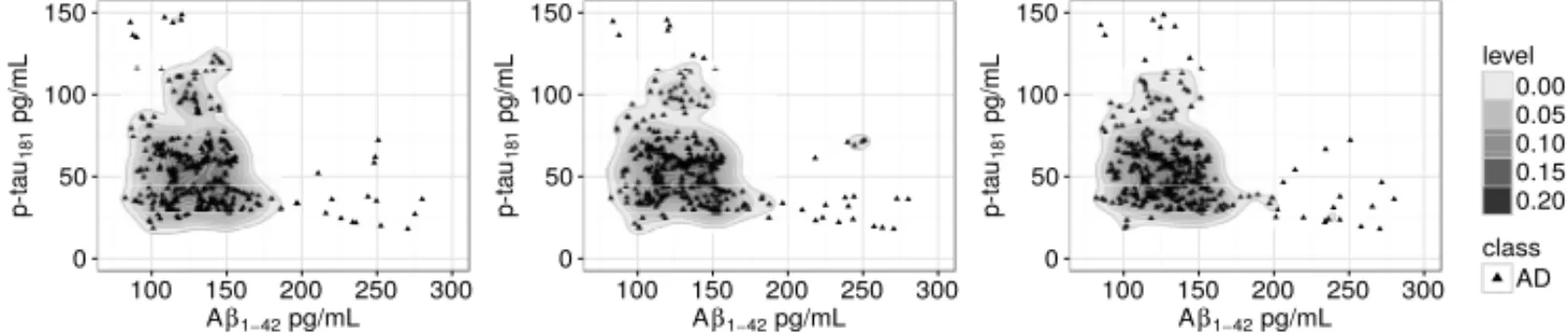
SMOTE is similar to kNN and can be implemented as follows [29]: first, a pattern in the mi-nor class is randomly selected, then, a synthetic pattern is included between a randomly chosen pattern in itsk-neighborhood, repeated the procedure until achieving desired prior. SMOTE in-creases the parameter space that must be searched to obtain the model with highest prediction rate. In this work, we set SMOTE’sk-neighborhood parameter ask =5. Figure 6 depicts how the amount of oversampling changes the distribution for 50% and 100% of synthetic data added in AD class relative to MCI class, usingk=5. The Bhattacharyya coefficient for 50% and 100% oversampling relative to the original distribution are 0.994579 and 0.9975564 respectively. Fig-ure 7 depicts the effect of parameterk in SMOTE algorithm. Fork =7, k = 15 andk = 30 the Bhattacharyya coefficient (assuming Gaussian distributions), from original sample is respec-tively, 0.9924127, 0.9972362 and 0.9935776, give that the value 1 means a complete distribution overlap.
0 50 100 150
100 150 200 250 300
Aβ1−42 pg/mL
p-tau
181
pg/mL
0 50 100 150
100 150 200 250 300
Aβ1−42 pg/mL
p-tau
181
pg/mL
0 50 100 150
100 150 200 250 300
Aβ1−42 pg/mL
p-tau
181
pg/mL
level 0.00 0.05 0.10 0.15 0.20
class AD
Figure 6: From left to right, the original data, synthetic oversampled 50% with original data, synthetic oversampled 100% with original data, respectively and their distributions.
0 50 100 150
100 150 200 250 300
Aβ1−42 pg/mL
p-tau
181
pg/mL
0 50 100 150
100 150 200 250 300
Aβ1−42 pg/mL
p-tau
181
pg/mL
0 50 100 150
100 150 200 250 300
Aβ1−42 pg/mL
p-tau
181
pg/mL
level 0.00 0.05 0.10 0.15 0.20
class AD
Figure 7: Original data with SMOTE oversampled 100% for values of parameterk, from left to right,k=7,k=15 andk=30.
2.4 Wrapper feature selection
correlation and information theoretical criterion [14]. As shown in [30] the optimal choice of features does not imply the choice of relevant features. Conversely, optimality does not imply in relevancy. For instance, features that are presumably redundant may enhance the precision when combined with useful features [14].
Despite the lack of guarantees presented, feature selection methods were invaluable to deal with high-dimensional real-world problems. Feature selection methods were initially designed to deal with classification problems with no more than 40 features [30], now they are able to deal with thousands of features. For instance, in classification problems related with genetics feature space dimensionality ranges from 6000 to 60000 [14] one can expect a strong effect of the curse of dimensionality. Such extreme problems have received attention uncovering the molecular mech-anisms related to AD [31] and have motivated initiatives like AlzGene focused on providing data resources for AD genetic research. Despite that, in this work, the feature selection techniques will be applied to at least 9 features in order to observe the group-wise probability of a feature being more relevant than other. Examples of feature selection techniques are feature extraction, feature construction, feature selection techniques for non-supervised learning, etc.
Feature selection methods are divided into three categories due to the relation with the classifier: filter, wrapper and embedded methods. Filters select a subset of features independently of the chosen classifier and the procedure mainly focus on ranking the features given defined criteria. Conversely, wrappers use classifiers’ measures as criteria to select subsets. Lately, embedded methods use a structured model to get the set of relevant features subject to a classifier [14]. For a complete discussion on the feature selection strategies and benefits see [14].
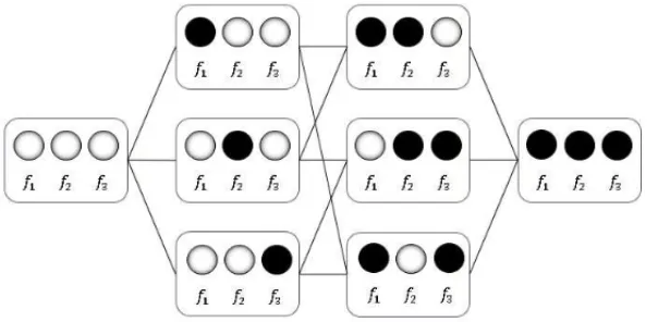
Here we compare three wrapper methods using the kNN classifier combined with SMOTE to select the most useful subset of features. The three wrapper methods compared are defined on the following search strategies: backward elimination, forward selection and hill-climbing se-lection [14]. The subset obtained using the three methods will be compared to all combinations of features in order to observe if they are able to reach the optimum subset drawn from the rank with all feature combinations. Additionally, a noise feature will be included in the fea-ture selection procedure in order to compare the feafea-tures to a non-significant case. In Figure 8 we depict an example of search graph with all possibilities for three combinations. Regarding Figure 8 we have that in the far left stage, no features chosen and the far right all features chosen. Backward elimination moves right to left; forward selection left to right; hill climbing moves to any direction.
Figure 8: Scheme showing how to choose a subset of 3 features, using forward selection, back-ward elimination, and hill-climbing.
combining two previous approaches. Here we set up hill-climbing starting from the empty set feature. All wrappers in this work are greedy algorithms and are subject to be trapped in a local maximum [30] (relative to the classification rate). A greedy algorithm can only optimize in a short distance and do not prevent that a good choice for a given iteration can lead to losing better options. There are search strategies designed to avoid this greedy drawback, for instance, the simulated annealing and the genetic algorithms [14].
2.5 Validation
Overfitting happens when the classifier’s prediction to the training phase are far better than the test phase [6]. The validation is appropriate to observe if the classifier is overfitted. An overfitted classifier cannot generalize results achieved in training phase for unseen patterns. Confusion matrix Pis a tool to assess the classifier outcomes and to interpret classification precision. The confusion matrix shows the class wise probability of classifyingx∗in the classωj given that it
was generated by classωi, for shortPi,j =p(x∗∈ωi|x∗∈ωj)= p(ωi|ωj). Furthermore, Pis
a stochastic matrix,
∀i c
j=1
p(wi|wj)=1 with p(wi|wj)≥0 for i,j =1, . . . ,c,
the Ptrace average is the probability of correct classifications for all classes or precision [18]. This measure defines a scalar magnitude that enables us to compare the many classifiers in the feature selection process. Furthermore, the 10-fold CV [6] is applied to the confusion matrices to obtain deviations of the feature’s subsets. The scalar for classifier’s comparisons can be written as,
val(P):=Rc×c→R val(P)=
c
i=1
P(wi|wi)
3 RESULTS AND DISCUSSION
Features for specific and general cohort studies owing to identify AD spectrum come from vari-ous sources: cognitive, genetic, neuroimaging, proteomic and others [16]. These features intend to provide insights on biological factors AD which is critical to understanding the disease pro-gression and to early prevention strategies [1]. Feature combinations provide higher classification rates than features by itself, also there are combinations more precise than others. For instance, a feature may confer a poor classification rate when many classes are included, even being highly valuable to understand AD biological processes, as depicted in Figure 4. This is, the combina-tion Aβ1−42andp-tau181, which sustain the main hypothesis for neurodegeneration [1] achieves
a precision of 42.29±1.32% and 43.40±4.61%, respectively for LOOCV and 10-fold CV for kNN withkoptimized and imbalanced data. Thus, it is necessary to find additional features or combinations to better identify AD. However, forn features the number of combinations is given byn
i=1i!(nn−!i)!, thus requiring strategies to avoid computational effort to uncover such
combinations. Wrapper feature selection techniques are suitable to avoid the comparison of all features combinations while maximizing a chosen classifier’s precision. In case, the kNN that allows the all-versus-all strategy to observe how the classes affect each other all at once. Also, the all-versus-all strategy contrasts to the binary adapted strategies that are widely used in AD research along with ROC analysis [1]. We compare the three techniques of wrappers feature selection to the global rank of features for each sampling strategies using confusion matrices. Moreover, Gaussian noise (mean=0, sd=1) was added to feature space in order to compare an irrelevant feature to the features displayed in Table 1, with label N (noise). The Table 2 shows the test performance of sorted combinations by higher classification rate among the non-defining features and by the number of features.
Excluding the defining features (3,5) most of the wrappers in this work were able to identify sub-optimal combinations given the precision of combinations available. For imbalanced dataset the combinations found are: 4,6 for hill climbing (position 2); 4,1,8 for backward elimination (position 28); 4,6,7,8 for forward selection (position 41). With random undersampling the com-binations found are: 4,6 for hill climbing (position 8); 1,4,6,8 for backward elimination (posi-tion 2); 4,1 for forward selec(posi-tion (posi(posi-tion 5). With oversampling (SMOTE) the combina(posi-tions found are: 4,6,7,8,N for hill climbing (position 38); 1,2,4,6,7,8,N for backward elimination (position 9); 4,7,6,8 for forward selection (position 21). All strategies of sampling and wrapper feature selection found sub-optimal combinations relative to the rank position. For the complete ranking list see on-line contents. One can notice that even with hill-climbing which combines the forward and backward strategies it can be trapped in local maximum and be affect by the cross-validation components. For instance, using oversampling with backward elimination was found the position 9 and combined with hill-climbing the position 38 in the full ranking list.
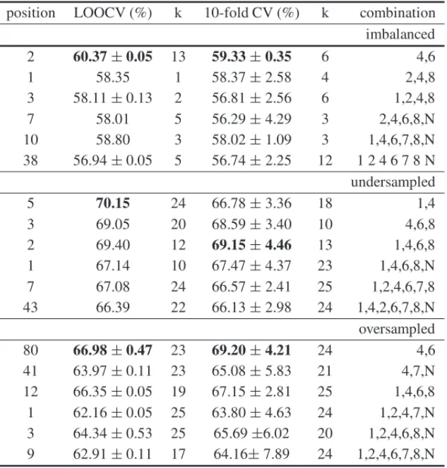
cross-Table 2: Rank of combinations for the three imbalanced strategies. Note the highest classification rate was bolded for each validation method.
position LOOCV (%) k 10-fold CV (%) k combination
imbalanced
2 60.37±0.05 13 59.33±0.35 6 4,6
1 58.35 1 58.37±2.58 4 2,4,8
3 58.11±0.13 2 56.81±2.56 6 1,2,4,8
7 58.01 5 56.29±4.29 3 2,4,6,8,N
10 58.80 3 58.02±1.09 3 1,4,6,7,8,N
38 56.94±0.05 5 56.74±2.25 12 1 2 4 6 7 8 N
undersampled
5 70.15 24 66.78±3.36 18 1,4
3 69.05 20 68.59±3.40 10 4,6,8
2 69.40 12 69.15±4.46 13 1,4,6,8
1 67.14 10 67.47±4.37 23 1,4,6,8,N
7 67.08 24 66.57±2.41 25 1,2,4,6,7,8
43 66.39 22 66.13±2.98 24 1,4,2,6,7,8,N
oversampled 80 66.98±0.47 23 69.20±4.21 24 4,6
41 63.97±0.11 23 65.08±5.83 21 4,7,N
12 66.35±0.05 19 67.15±2.81 25 1,4,6,8
1 62.16±0.05 25 63.80±4.63 24 1,2,4,7,N
3 64.34±0.53 25 65.69±6.02 20 1,2,4,6,8,N
9 62.91±0.11 17 64.16±7.89 24 1,2,4,6,7,8,N
validation process and results may vary when the random generator number is unfixed. This variation ranges between the very first combinations to the middle-rank combinations. The list of 502 combinations for each technique to aid imbalance is available on-line, also the 120 combi-nations rank for non-defining features and the 26 combicombi-nations rank for non-cognitive features.
20 24 28
0 4 8
CDRSB
MMSE
20 24 28
0 4 8
CDRSB
MMSE
20 24 28
0 4 8
CDRSB MMSE probability 0.00 0.25 0.50 0.75 1.00 class AD CN MCI
Figure 9: Decision region for balanced (undersampled) three class problem solved with 5NN. From left to right, decision regions of CN, MCI and AD, respectively. Note that even for the defining features there is some errors.
classified as CN is 35.6%. Also, in Figure 10 the confusion matrices for balanced problems (2nd
and 3rd rows) show that the major class (MCI) have more classification errors than the minor classes (CN, AD). Conversely, in the imbalanced problem, the confusion matrices (1st row) for the major class are more precise and the minor class has more misclassification errors. This result is expected and can be used to control the compromise between class resampling in order to achieve a balance that minimizes the classification error.
AD MCI CN AD MCI CN 84 4.3 0 16 77 35.6 0 18.5 64.3
AD MCI CN AD MCI CN 80 3.1 0 19.9 83.4 30.6 0 13.4 69.3
AD MCI CN AD MCI CN 76.9 3.6 0 23 86.3 33.1 0 10 66.8
AD MCI CN AD MCI CN 85 3.1 0 14.9 87.5 23.7 0 9.2 76.2
AD MCI CN AD MCI CN 83 3.1 0 17 90 16.8 0 6.8 83.1
AD MCI CN AD MCI CN 92 2.4 0 8 92.6 12.5 0 4.8 87.5
AD MCI CN AD MCI CN 88 3.6 0 12 94.3 8.7 0 1.9 91.2
AD MCI CN AD MCI CN 84 2.6 0 15.9 97.3 6.2 0 0 93.7
AD MCI CN AD MCI CN 94 9.5 0 6 51.7 13.7 0 38.7 86.2
AD MCI CN AD MCI CN 95 6.8 0 5 58.2 11.8 0 34.8 88.1
AD MCI CN AD MCI CN 96 7.5 0 4 61.7 6.2 0 30.7 93.7
AD MCI CN AD MCI CN 95 7.8 0 5 69.2 8.7 0 22.9 91.2
AD MCI CN AD MCI CN 94 6 0 6 71.9 6.8 0 21.9 93.1
AD MCI CN AD MCI CN 99 7 0 1 74.6 6.2 0 18.2 93.7
AD MCI CN AD MCI CN 97 6 0 3 84.1 6.2 0 9.7 93.7
AD MCI CN AD MCI CN 90 7 0 10 91.9 5.6 0 0.9 94.3
AD MCI CN AD MCI CN 90 7.8 0 9.9 63.1 15 0 29 85
AD MCI CN AD MCI CN 93 6.8 0 6.9 66 12.5 0 27 87.5
AD MCI CN AD MCI CN 93 6.3 0 6.9 69 8.7 0 24.6 91.2
AD MCI CN AD MCI CN 93 6.8 0 6.9 77.3 10.6 0 15.8 89.3
AD MCI CN AD MCI CN 95 5.8 0 5 78.5 7.5 0 15.6 92.5
AD MCI CN AD MCI CN 95 5.3 0 5 79 3.7 0 15.6 96.2
AD MCI CN AD MCI CN 92 6.3 0 8 93.6 6.2 0 0 93.7
AD MCI CN AD MCI CN 90 5.1 0 10 91.4 10 0 3.4 90
Figure 10: By row is depicted the confusion matrices for imbalanced, undersampled and over-sampled combinations, respectively. Each column depicts from 8t h to 1st ranked combinations in the 502 rank (on-line contents).
can be interested in the probability of combinations that contain the feature 2 and not 8 to provide higher precision than combinations containing 8 and not 2, the left matrix in Figure 11 shows that is 38.7%. However, the matrices are not symmetrical due to some combinations have the same classification rate and due to round-off error. As argued by [1] the neuropsychological tests are more precise and standardized measures to detect AD. Figure 11 shows only non-cognitive features (1,2,7,8). Despite neuropsychological tests being cost-effective biomarkers and its com-binations provide a high precision, they do not provide information on the biological mechanism of AD. The suggestion of how they provide a higher precision is due to the limited possibilities of outcomes that define the neuropsychological scores, leading to overlaying patterns, as repre-sented in Figure 9. This is, biomarkers that have fractional values are less subject to becoming an integer value grid in comparison to neuropsychological tests. In the right matrix of Figure 11 the noise has a higher probability in average to increase the classification rate than proteomic biomarker 7 however it does not mean irrelevancy [14]. As argued by [14], a feature that is supposed to be irrelevant could contribute to enhancing the classifier performance.
1 2 7 8 N A
1 2 7 8 N A 0 0 0 0 0 0 100 0 51 61.2 36.7 62.2 100 46.9 0 59.1 40.8 61.7 100 38.7 40.8 0 26.5 51.5 100 61.2 59.1 73.4 0 73.4 100 36.7 37.7 48.4 26 0
1 2 7 8 N A
1 2 7 8 N A 0 0 0 2 0 0.5 100 0 53 48.9 46.9 62.2 100 46.9 0 42.8 38.7 57.1 97.9 51 57.1 0 42.8 62.2 100 53 61.2 57.1 0 67.8 99.4 37.7 42.8 37.7 32.1 0
1 2 7 8 N A
1 2 7 8 N A 0 30.6 28.5 28.5 32.6 30.1 69.3 0 42.8 42.8 44.8 50 71.4 55.1 0 48.9 51 56.6 71.4 57.1 48.9 0 51 57.1 67.3 53 44.8 44.8 0 52.5 69.8 48.9 41.3 41.3 44.8 0
Figure 11: From right to left, probability matrix of a feature to provide higher classification rate than others for the imbalance, undersampled and oversampled, ranks respectively. Label “A” stands for column-wise and row-wise average.
wkNN. Despite the curse of dimensionality that affects kNN more than SVM and wkNN, the kNN with SMOTE achieves higher precision in average compared to these methods without bal-ance aids. For the canonical biomarkers combination, Aβ1−42and p-tau181, the SVM reaches
33.34±0.68% and the wkNN reaches 37.36±3.02%.
4 CONCLUSION
Wrappers techniques for feature selection have shown to be efficient to find the suboptimal combinations given by the rank for all imbalance aid strategies for the proposed problem. How-ever, adding more features to test limits of greedy search could be less successful. Including features is challenging because it increases the number of patients who did not undergo to all examinations. This can be seen in the complete dataset available in ADNI. Fortunately, kNN inspired data missing techniques are available and would be useful to identify more precise com-binations that include interpretation benefits for AD mechanisms. However, to deal with im-provements to kNN which imply in non-convex optimizations will require more studies. There are options to increase kNN performance such as metric learning [28] and normalization strate-gies [21]. However, this will increase the parameter space to optimize and improvements in the computation performance. Even with the curse of dimensionality, the kNN with SMOTE over-come in average SVM and wKNN in reproducing the definition. However, the benefits of data balance would increment any classifier precision. The performed all-versus-all strategy requires less classifiers to be built than binary strategies. The class defining features (labels 3,5) increase artificially the class combinations for rank with 502 possibilities, however, it was useful to obtain a comparative. Comparisons using non-cognitive features reveal that FDG contributes more to increase the classification rate. However, more non-cognitive features are needed to observe if dominance for FDG holds, this is a challenge given mentioned data issues for missing values and data imbalance.
ACKNOWLEDGMENTS
Data collection and sharing for this project was funded by the ADNI (National Institutes of Health Grant U01 AG024904) and DOD ADNI (Department of Defense award number W81XWH-12-2-0012). The author thanks CAPES for the master’s scholarship provided.
desba-lanceados. Uma vez que o n´umero de combinac¸˜oes biomarcadores ´e fatorial ent˜ao usamos wrappers para evitar as m´ultiplas comparac¸˜oes. Neste trabalho comparamos a capacidade de trˆes t´ecnicas wrapper de selecc¸˜ao de caracteristicas na obtenc¸˜ao de combinac¸˜oes de biomar-cadores ao maximizar taxas de classificac¸˜ao. Al´em disso, como crit´erio para os wrappers usamos o classificadork-vizinhos mais pr´oximos com preprosessamento de balanc¸o de da-dos, sobreamostragem aleat´oria e sobamostragem (SMOTE). Em geral nossa an´alise mostra como as combinac¸˜oes de biomarcadores s˜ao afetadas pela estrat´egia de equil´ıbrio de dados. Mostramos que os biomarcadores n˜ao-definidores de classe e n˜ao-cognitivos tˆem menos precis˜ao do que as medidas cognitivas para classificar AD. A nossa abordagem supera em m´edia os classificadores m´aquina de vetores de suporte ek-vizinhos mais pr´oximos ponde-rado com 94,34±3,91% de precis˜ao para biomarcadores que definem a classe.
Palavras-chave: k-vizinhos mais pr´oximos, SMOTE, selec¸˜ao de caracter´ısticas, biomar-cadores de Alzheimer, problema de classificac¸˜ao.
REFERENCES
[1] M.S. Fiandaca, M.E. Mapstone, A.K. Cheema & H.J. Federoff. The critical need for defining preclin-ical biomarkers in Alzheimer’s disease.Alzheimer’s & Dementia,10(3) (2014), S196–S212. [2] C.R. Jack, D.S. Knopman, W.J. Jagust, L.M. Shaw, P.S. Aisen, M.W. Weiner, R.C. Petersen & J.Q.
Trojanowski. Hypothetical model of dynamic biomarkers of the Alzheimer’s pathological cascade. The Lancet Neurology,9(1) (2010), 119–128.
[3] R.A. Sperling, P.S. Aisen, L.A. Beckett, D.A. Bennett, S. Craft, A.M. Fagan, T. Iwatsubo, C.R. Jack, J. Kaye & T.J. Montine et al. Toward defining the preclinical stages of Alzheimer’s disease: Recom-mendations from the national institute on aging-Alzheimer’s association workgroups on diagnostic guidelines for Alzheimer’s disease.Alzheimer’s & dementia,7(3) (2011), 280–292.
[4] A.A. Motsinger-Reif, H. Zhu, M.A. Kling, W. Matson, S. Sharma, O. Fiehn, D.M. Reif, D.H. Ap-pleby, P.M. Doraiswamy & J.Q. Trojanowski et al. Comparing metabolomic and pathologic biomark-ers alone and in combination for discriminating Alzheimer’s disease from normal cognitive aging. Acta neuropathologica communications,1(1) (2013), pp. 28.
[5] S.J. Teipel, O. Sabri, M. Grothe, H. Barthel, D. Prvulovic, K. Buerger, A.L. Bokde, M. Ewers, W. Hoffmann & H. Hampel. Perspectives for multimodal neurochemical and imaging biomarkers in Alzheimer’s disease.Journal of Alzheimer’s Disease,33(s1) (2013), S329–S347.
[6] C.M. Bishop. Pattern Recognition and Machine Learning (Information Science and Statistics). Springer, (2007).
[7] T. Fawcett. An introduction to roc analysis.Pattern recognition letters,27(8) (2006), 861–874. [8] L. Khedher, J. Ram´ırez, J.M. G´orriz, A. Brahim, F. Segovia & A.D.N. Initiative et al. Early diagnosis
of Alzheimer’s disease based on partial least squares, principal component analysis and support vector machine using segmented mri images.Neurocomputing,151(2015), 139–150.
[10] Q. Yang & X. Wu. 10 challenging problems in data mining research.International Journal of Infor-mation Technology & Decision Making,5(04) (2006), 597–604.
[11] H. He & E.A. Garcia. Learning from imbalanced data.IEEE Transactions on knowledge and data engineering,21(9) (2009), 1263–1284.
[12] B. Krawczyk. Learning from imbalanced data: open challenges and future directions.Progress in Artificial Intelligence, (2016), 1–12.
[13] C. Humpel. Identifying and validating biomarkers for Alzheimer’s disease.Trends in biotechnology,
29(1) (2011), 26–32.
[14] I. Guyon & A. Elisseeff. An introduction to variable and feature selection.Journal of machine learn-ing research,3(Mar) (2003), 1157–1182.
[15] Y. Saeys, I. Inza & P. Larra ˜naga. A review of feature selection techniques in bioinformatics. Bioinfor-matics,23(19) (2007), 2507–2517.
[16] K. Lopez-de Ipi˜na, J.B. Alonso, J. Sol´e-Casals, N. Barroso, P. Henriquez, M. Faundez-Zanuy, C.M. Travieso, M. Ecay-Torres, P. Martinez-Lage & H. Eguiraun. On automatic diagnosis of Alzheimer’s disease based on spontaneous speech analysis and emotional temperature.Cognitive Computation,
7(1) (2015), 44–55.
[17] A. Sarica, G. Di Fatta, G. Smith, M. Cannataro & J.D. Saddy et al. Advanced feature selection in multinominal dementia classification from structural mri data, inProc MICCAI Workshop Challenge on Computer-Aided Diagnosis of Dementia Based on Structural MRI Data, pp. 82–91 (2014). [18] J.S. Marques.Reconhecimento de Padr ˜oes: m´etodos estatist´ıcos e neuronais. IST press (2005). [19] T. Tapiola, I. Alafuzoff, S.-K. Herukka, L. Parkkinen, P. Hartikainen, H. Soininen & T. Pirttil¨a.
Cere-brospinal fluidβ-amyloid 42 and tau proteins as biomarkers of Alzheimer-type pathologic changes in the brain.Archives of neurology,66(3) (2009), 382–389.
[20] A.W. Toga & K.L. Crawford. The Alzheimer’s disease neuroimaging initiative informatics core: A decade in review.Alzheimer’s & Dementia,11(7) (2015), 832–839.
[21] C.-M. Ma, W.-S. Yang & B.-W. Cheng. How the parameters ofk-nearest neighbor algorithm im-pact on the best classification accuracy: In case of parkinson dataset.Journal of Applied Sciences,
14(2) (2014), 171–176.
[22] A. Bhattacharyya. On a measure of divergence between two multinomial populations.Sankhy ¯a: the indian journal of statistics,7(4) (1946), 401–406.
[23] L. Devroye, L. Gy¨orfi & G. Lugosi.A probabilistic theory of pattern recognition,31. Springer Science & Business Media,31(2013), 638 pages.
[24] G. Bhattacharya, K. Ghosh & A.S. Chowdhury. An affinity-based new local distance function and similarity measure for knn algorithm.Pattern Recognition Letters,33(3) (2012), 356–363.
[25] T.M. Cover & P.E. Hart. Nearest neighbor pattern classification.Information Theory, IEEE Transac-tions on,13(1) (1967), 21–27.
[26] T. Bailey & A.K. Jain. A Note on Distance-Weightedk-Nearest Neighbor Rules.IEEE Transactions on Systems, Man, and Cybernetics,SMC-8(4) (1978), 311–312.
[28] C.C. Aggarwal, A. Hinneburg & D.A. Keim. On the surprising behavior of distance metrics in high dimensional space, inInternational Conference on Database Theory, Springer, (2001), 420–434. [29] N.V. Chawla, K.W. Bowyer, L.O. Hall & W.P. Kegelmeyer. Smote: synthetic minority over-sampling
technique.Journal of artificial intelligence research,16(2002), 321–357.
[30] R. Kohavi & G.H. John. Wrappers for feature subset selection.Artificial intelligence,97(1) (1997), 273–324.