Braz. J. Phys. vol.33 número2

Simulations of Plasmas with Electrostatic PIC

Models Using the Finite Element Method

A. C. J. Paes, N. M. Abe, V. A. Serr˜ao, and A. Passaro

12231-970, S˜ao Jos´e dos Campos, S˜ao Paulo, Brazil

Received on 20 June, 2002. Revised version received on 10 November, 2002

Particle-in-cell (PIC) methods allow the study of plasma behavior by computing the trajectories of finite-size particles under the action of external and self-consistent electric and magnetic fields defined in a grid of points. In this work, the Finite Element Method (FEM) is used in order to obtain the self-consistent fields. An electro-static PIC-FEM computational code for simulation of one-dimensional (1D) and two-dimensional (2D) plasmas was developed based on two available and independent codes: the first one a 1D PIC code that uses the Finite Difference Method and the other a FEM code developed at the Instituto de Estudos Avancados (IEAv). The Poisson equation is solved and periodic boundary conditions are used. The ion background that neutralizes the total plasma charge is kept fixed and uniformly distributed in the domain of study. The code is tested by study-ing the fluctuations of the plasma in thermal equilibrium. In thermal equilibrium a plasma sustain fluctuations of various collective modes of electrostatic oscillations, whose spectral distribution can be analytically obtained by using the fluctuation-dissipation theorem and the Kramers-Kronig relation. In both 1D and 2D cases, there are excellent agreement between the spectral distribution curves predicted theoretically and those obtained by simulation for finite size particles and long wavelengths.

I

Introduction

In this work, we use the particle-in-cell (PIC) model, orig-inated from the work of J.M. Dawson [1, 2, 3] in the late fifties, for the simulation of plasmas. In this model, the plasma is represented by thousands of particles (actu-ally macroparticles, since each particle used in the simula-tion represents thousands of particles of a real experiment). From the positions and velocities of these particles at a cer-tain instant, we calculate the current and charge densities us-ing one of various schemes of particle distribution to a grid of points. The grid spacing∆xmust be sufficiently small to resolve the collective behavior of plasmas (typically∆xof the order of the Debye lengthλDe).

Using these charge and current densities, we calcu-late the self-consistent electric and magnetic fields via Maxwell’s equations. Then, with these fields plus the ex-ternally applied ones, we obtain the new particle positions and velocities. Finally, we proceed along this basic cycle with a∆tsufficiently small to resolve the highest frequency of the problem (typically the plasma frequencyωpe).

In the PIC code, Maxwell’s equations are usually solved by the Finite Difference Method (FDM) or by Fourier tech-niques (specially when periodic boundary conditions are in-volved). In the FDM, the fields are defined in a grid of points, the derivatives are replaced by differences in the val-ues of the field in adjacent grid points, and difference equa-tions on the grid substitute the differential field equaequa-tions.

Another approach is to apply the Finite Element Method (FEM) instead of FDM to solve the Maxwell’s equations. In FEM, the system is divided into subsystems of simple ge-ometry (for example, triangles and/or rectangles for a two-dimensional program), which are called finite elements. In-side each element, the values of the fields are calculated by means of interpolation functions, for example polyno-mials. The shape of the interpolation in the elements is de-fined by field values, and sometimes its derivatives, at the nodal points. The field derivatives are obtained by deriv-ing the interpolatderiv-ing functions, and the field equations are approximated by minimizing integral (integro-differential) equations obtained by variational principles or by applying the weighted residual method to the differential equations and boundary conditions.

The FEM has advantages in treating elliptic and parabolic equations when compared with the FDM. The as-sociation of boundary conditions to nodal points, mesh re-finement, and the adoption of different mesh types (mixed-mesh) become easy in the finite element method. Moreover, the finite element method has advantages of optimization and accuracy [4]. A short description of FEM is presented in section II.

developed the computational program based on two inde-pendent codes. The first one is a 1D PIC modeling software developed by Kruer [5]. This code uses the Finite Differ-ence Method (FDM) in order to compute the self-consistent field. The second one is a 1D and 2D FEM code fully de-veloped at the Instituto de Estudos Avancados (IEAv). In section II, we present the numerical method used. In section III, we present some results of the simulations in the 1D and 2D cases, and deduce expressions that allow us to compare the simulation results with the theoretical ones. Finally, in section IV we present some conclusions.

II

Numerical model

In particle simulation, we attempt to study the behavior of plasmas by following the motion of a great number of parti-cles. Since it is too expensive to compute the self-consistent motion of the plasma by calculating the force on each parti-cle due to every pair interaction, a spatial grid is introduced on which the charge and current density are accumulated; electric and magnetic fields are stored in the grid as well.

In this work, we adopt an electrostatic model, i.e., only electric fields are considered. The basic scheme of this model is very simple. First, we accumulate the charge den-sity on the grid from particle positions and velocities. Sec-ond, we solve Poisson’s equation on the grid to find the elec-tric potential and the elecelec-tric field. Finally, we interpolate the electric field on the grid to the particles position and use the interpolated force on Newton’s equations of motion to determine new particle positions and velocities. Then, we repeat this cycle as many time steps as necessary to study our system.

Numerous algorithms are available for the charge accu-mulation process in the spatial grid, such as NGP (nearest grid point) and PIC (particle-in-cell) [6]. In this work, we are using the PIC modeling. In this method, a point charge atxi is assigned to its nearest grid points by using a

lin-ear interpolationW(x). Particle pushing is done with the second-order accurate leap-frog technique.

The electrostatic field generated by a certain charge dis-tribution can be obtained from the solution of Poisson’s equation:

∇2Φ(~r) = ρ(~r), (1) with boundary conditions:

Φ = φs, inΓ1, (2)

and

∂Φ

∂n =fs inΓ2 (3)

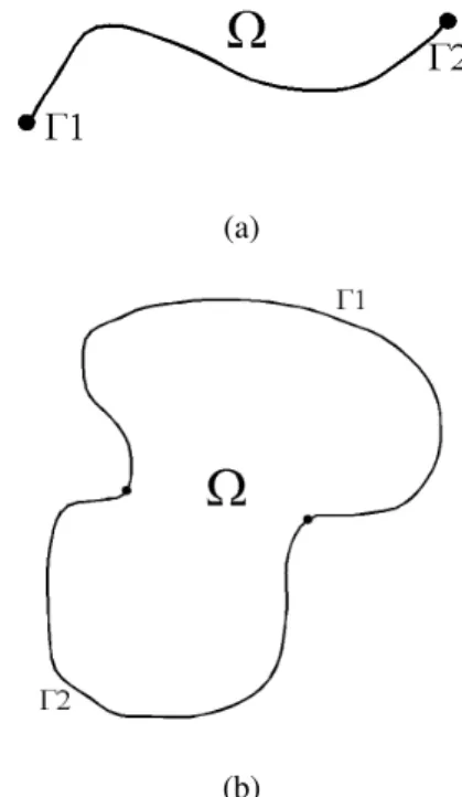
where Γ = Γ1 + Γ2 is the surface that delimits the

do-main of study Ω. Fig. 1 shows the domain and delimit-ing surfaces for both a one-dimensional (1D) and a two-dimensional (2D) domain.

(a)

(b)

Figure 1. Limiting surfacesΓ1andΓ2for (a) a one-dimensional domain and (b) a two-dimensional domain.

An approximated solution φ for the differential equa-tion (1) can be obtained by applying the Weighted Residual Method (WRM). A complete description of this method can be obtained in several basic literature on the FEM [7, 8]. In WRM, the integral of the residueIover the entire domainΩ

is imposed equal to zero:

I= Z

Ω

P1R1dΩ +

Z

Γ1

P2R2dS+

Z

Γ2

P3R3dS= 0 (4)

with:

R1=∇2φ(~r)− ρ(~r) (5)

R2=φ −φs (6)

R3= ∂φ

∂n−fs. (7) The time independent weighting functions,P1,P2, andP3,

are chosen arbitrarily. Only one condition must be imposed on these weighting functions: they must be sufficiently reg-ular in order to obtain finite integrals.

By applying the first Green’s identity to equation 4, re-sults:

⌋

Z

Ω

− →

∇P1−→∇φ dΩ−

Z

Ω

P1ρ dΩ +

Z

Γ1

P1−→n ·−→∇φ dS+

Z

Γ2

Z

Γ1

P2(φ−φs)dS+

Z

Γ2

P3

µ

fs−

∂φ ∂n

¶

dS= 0. (8)

The fifth integral can be eliminated by imposing that the solution satisfies identically the Dirichlet boundary condition inΓ1.

As the weighting functions are arbitrary,P1is chosen equal to zero inΓ1, resulting:

Z

Ω

− → ∇P1

− → ∇φ dΩ−

Z

Ω

P1ρ dΩ +

Z

Γ2

P3fsdS+

Z

Γ2

(P1−P3)

∂φ

∂ndS= 0. (9)

⌈

Without loss of generality,P3is chosen equal toP1, in

order to eliminate the fourth integral in (9). Additionally, in this work the Neumann condition inΓ2is always

homoge-neous, e.g., fs = 0(there is no electric current applied in

the domain of study).

The resulting integral equation:

Z

Ω

− → ∇P1

− → ∇φ dΩ−

Z

Ω

P1ρ dΩ = 0 (10)

represents the weak formulation for the Poisson equation [7, 8]. We apply the FEM in order to evaluate Eq.(10) .

Figure 2. A triangular finite element mesh for an arbitrary domain.

In the FEM, the domainΩis subdivided into elements of simple geometry, such as, lines and curves in 1D simu-lations, triangles and rectangles for 2D simusimu-lations, tetrahe-dra, parallelepipeds, and prisms for three-dimensional (3D) simulations. Each element defines a subdomain namedΩγ_.

The Fig. 2 illustrates a triangular mesh for an arbitrary do-main of study. These elements of simple geometry, named finite elements, must obey the following rules in order to constitute a consistent mesh:

- the sum of the area of each element results in the do-main area

Ã

S

γ=1...N E

Ωγ _{= Ω}

!

; and

- the elements do not intersect each other

Ã

T

γ=1...N E

Ωγ_{= 0}

!

. NE is the number of elements in which the domain is decomposed.

The finite element mesh follows all boundaries of the geometric model even for a complex geometry. Due to this characteristic, the attribution of boundary conditions to the mesh points is easier than in the FDM, because it is not nec-essary to treat mesh points that do not coincide with the ge-ometric lines.

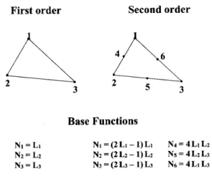
Inside each element, the approximated value of the de-pendent variable is calculated from a finite set of linearly independent base functions (compact support). This set de-pends on the family and approximation order of the used elements. Fig. 3 shows two examples of the triangular ele-ments family and the base function set for each case. The functions L1, L2, and L3are given by:

Li=

ai+bix+ciy

2∆

where∆is the area of the triangle and the coefficients a, b, and c are obtained from the coordinates of the vertices of the triangle:

ai=εijk(xjyk−xkyj)

bi=εijk(yj−yk)

ci=εijk(xk−xj)

εijkis the three-dimensional Levi-Civitta symbol [9]. The

indices i, j, and k vary from 1 to 3.

The derivation of these expressions for triangular ele-ments and for eleele-ments of other families is presented in [7]. In general, the shape of the interpolation functions in the element is defined by the values of the dependent vari-ables and, sometimes, their derivatives, in some points of the element, the nodal points. The dependent variables, and, when necessary, their derivatives, are named nodal vari-ables. Thus, one or more nodal variables are computed in each nodal point. The number of nodal variables depends on the formulation adopted for the solution of a given prob-lem. In the formulation adopted in this work, there is only one nodal variable: the electric potential.

In this way, the scalar potential in a elementγis written as a sum of the base functionsN_i(γ):

φ(γ)(~rj) = N

(γ)

i (~rj)φ

(γ)

i , i= 1, ....n0 (11)

whereφ(_iγ)are the potential values on the nodal point i and n0is the number of nodal points of the element. Notice that

we are using the summation convention. The base functions have the following properties on the nodal points:

N_i(γ)(~rj) = δij (12)

whereδijis the Kronecker’s delta. This means that the base

functions assume the value one when the index of the nodal point, j, coincides with the index of the base function, i, and is zero in any other nodal point. The base functions for a de-termined element are valid only in the limits of this element. In the FEM, we also let the integro-differential equation (10) be equal to zero for each element, which allows us to write them individually:

Z

Ωγ

− →

∇P₁(γ).−→∇φ(γ)_dΩ−Z Ωγ

P₁(γ)ρ(γ)_{dΩ = 0}

(13)

whereΩγ_{corresponds to the element domain.}

In order to solve the residual equation, we have only to choose convenient weighting functions. In the finite el-ements approximation, inside each element the number of unknowns is equal to that of nodal variables. Consequently, we must choose the same number of weighting functions. The weighting functions inside each element coincide with the base functions used to describe the dependent variables (Galerkin’s method):

P_i(γ) = N_i(γ) (14) resulting for the residue equation in each element:

µZ

Ωγ

− → ∇Ni(γ).

− →

∇Nj(γ)dΩ

¶

φj−

Z

Ωγ

Ni(γ)ρ(γ)dΩ = 0

(15) with i = 1,2,...,n0.

A matricial notation can be used to represent the integral equation set (15):

[K]{φ}T = {b}T (16)

where:

[K] = Z

Ωγ

[gradN]T[gradN]dΩ (17)

{φ}=©

φ1 φ2 φ3 · · · φn0

ª

(18)

{b}= Z

Ωγ

{N}ρ(γ)dΩ (19)

{N}=©

N1 N2 N3 · · · Nn0

ª

(20)

[gradN] = 

 

∂{N}

∂x1

∂{N}

∂x2

· · ·





, (21)

andxistands for the ithcoordinate in a k-dimensional space.

For example, for the one-dimensional case, we use a lin-ear element in first order approximation (two nodal points, which correspond to the vertices of the line element), with linear interpolation functions given by:

N1(x) =

x12−x

l (22)

N2(x) =

x−x11

l (23)

in which

x11 : is the coordinate of the left nodal point,

x12 : is the coordinate of the right nodal point,

l :is the length of the element, x :is the coordinate inside the element, and the following matrices for the element:

[grad N] = [∂{N}

∂x ] =

1

l [−1 1], (24)

[K] = 1

l2

Z ·

1 −1

−1 1 ¸

dΩ = 1

l

·

1 −1

−1 1 ¸

,

(25)

{b} = Z

{N}ρ dΩ = lρ

2 [1 1]. (26)

After the calculation of the matrices of each element, we assemble the global system, i.e., the matricial system in-cluding all the nodal points. Because to each nodal point is associated a unique identification number in the system, the process of assemblage is simple. Each finite element matrix connects the set of nodal points of the element, and hence the values calculated for an element of the matrix can be added directly in the global matrix in the positions indicated by the number of the nodal points. An elegant mathemati-cal treatment of the global matrix assemblage is presented in [8]. The global matricial system is given by:

where[KG]is a symmetric and sparse matrix, of order NP x

NP (NP is the total number of nodal points of the grid). The vectors{φG}and{bG}have dimension NP.

The electric potential on the grid is obtained by solv-ing (27). In this work, we adopted the ICCG (Incomplete Cholesky Conjugate Gradient) method [10] to solve the sys-tem, because the matrix [KG] is sparse, real, and positive

definite.

III

Results

In this section, we show the results of simulations obtained with the developed electrostatic PIC-FEM (1D and 2D) nu-merical code. We applied the code to the study of fluctua-tions in a stable plasma.

Even in a Maxwellian plasma, there are fluctuations. Plasma waves are Cerenkov-emitted and Landau-damped. The balance between emission and absorption leads to thermal-level field fluctuations.

In spite of Vlasov theory and particle models simu-late collisionless plasmas, electric field fluctuations do not emerge from a Vlasov model because these fluctuations are connected in a basic way with the discreteness of the plasma. Consequently, particle models have to be used to calculate such fluctuations.

In order to obtain the electric field energy fluctuation spectrum theoretically, the test-particle picture is used [11]. In this model, it is considered the motion of a test charge in the Vlasov fluid (plasma described by the Vlasov equation). After some time, the test particle polarizes the plasma, that is, the particle get “dressed”. This means that in a plasma, the Coulomb potential (potential of interaction between par-ticles in vacuum) is modified because of collective effects, each negative charge attracts a cloud of positive charges and vice versa. From this potential and the corresponding den-sity fluctuation, the spectral distribution E2

k of the electric

field can be obtained (k stands for k-space, or Fourier space). At present, experiments are being conducted to ob-serve the process of particle “dressing” in a non-equilibrium plasma. This process has a predicted time scale of the order of(ωpe/2π)−1, which corresponds to 70 femtoseconds for

a plasma with density of2 1018_cm−3_{. The precision of the}

existing models can be verified by using pulsed lasers last-ing 27 femtoseconds to probe the plasma [12, 13]. However, for a Maxwellian plasma there is a well established result for the spectral distribution of the averaged longitudinal electric field energy given by [14]:

¿

E2

kL

8π

À = Te

2 1 1 +k2_λ2

De

(28)

for a system of lengthLand transverse area equal to one.Te

is the electron temperature in energy units.

This result can also be analytically obtained using the fluctuation-dissipation theorem and the Kramers-Kronig’s relation [4].

To compare this result deduced for a test charge (point electron) with the results of our simulations, we must re-member that we are simulating the physics of a plasma of finite-size macroparticles. The finite-size effects are un-avoidably associated with the interpolation function used to relate quantities to the grid. The macroparticle effect is due to the fact that each simulation particle represents thousands of electrons in a real experiment.

It can be shown that in k-space the charge density for a finite-size particle simply equals the charge density for a point particle system multiplied by a shape factorS(k). Thus, we can rewrite most of the plasma theory for the finite size particle system by replacing the chargeqbyqS(k)[4]. However, here, there is an additional difficulty since there are really two sources for the “finite-sizeness” of the particles. One is the above mentioned use of an interpola-tion funcinterpola-tionW(x)to relate particle quantities to the grid. This can never be avoided in a PIC code. A second pos-sible source is the use of various kinds of filter functions S(x), either in real space or k-space. The effective par-ticle shape is then the convolution of these two functions

R

W(x)S(x−x′_{)dx, or in k-space,W(k)S(k)[15].} The considerations above imply that we have to modify the termk2_λ2

De in Eq. (28) in order to take into account

finite-size effects. But macroparticle effects also lead to al-teration of Eq.(28). This modification comes from the fact that the temperature used in the formula must not be that of the electron, because in the statistical basis of Eq. (28), what matters is the freedom of kinetic motion. In the simu-lation, the free random motion is not assigned to an electron of energy 1₂mev2e (where me is the electron mass, andve

its velocity), but to a macroscopic particle of energy1₂mpv2p

(where mp is the macroparticle mass andvp its velocity).

Therefore, we should interpret Teas Tp =< 1₂ mpv2p >,

withTpthe macroparticle temperature (in units of energy).

Based on all the above considerations, the theoretical ex-pression for the spectral distribution of the averaged lon-gitudinal electric field energy for a plasma of finite-size macroparticle can be written:

¿

E2

kL

8π

À = Tp

2 µ

1 + k

2_λ2

De

S2_(k)W2_(k)

¶−1

. (29)

In this work, we compare the results of our simulations with this expression.

We know all terms of Eq. (29) but one. The unknown term isS(k)(sinceW(k)is obtained fromW(x), the pre-scribed interpolation function), that is, the filtering term.

In order to determine this filter, let us consider a sim-ple problem, that is, the normalized one-dimensional Gauss’ law∇xEx =ρ. In the theoretical case, applying a Fourier

transform to this equation we obtain Exk =

ρk

ikx

the electric field, because in this case they use a prescribed S(k)given bye−k2a2

2 ( withaof the order ofλ

De) filtering

out the short-wavelength (ka > 1) modes, lowering the ef-fective collision frequency, and thus allowing realistic sim-ulations with fewer particles. In this case they have for the one-dimensional Poisson equation:

Exk =

ρkS(k)

ik = ρke−

k2a2

2

ik (31)

with the wavenumberk=kx.

In our case, applying the finite element formulation for a Fourier mode, we have from the one-dimensional Poisson’s equation

Exk =

∆x sin(k∆x)ρk

i4sin(k∆x

2 )

. (32)

Comparing this expression with Eqs. (30) and (31) per-mits us to determineS(k)for our case, which is given by (for the normalized case∆x = 1):

S(k) = sin(k)k 4sin(k

2)

(33)

Figure 4. The filtering effect of the factor that multipliesρk(Eq.32)

for the finite element method (similar to the finite difference case [5]) and for the Fourier transform method [16], compared to the theoretical result.

In Fig. 4, we present the terms multiplyingρk(in fact the

log10of these terms) in the one-dimensional Poisson’s

equa-tion for the theoretical model, for the finite element method (similar in this case to the finite difference case referred to as Kruer’s case [5]), and for the Fourier transform method (re-ferred to as Decyk’s case [16]). The figure shows the filter-ing effect mentioned above, since the terms associated with FEM and Fourier transform decrease with k when compared with the theoretical result. Actually, the deducedS(k), Eq. (33), acts as an unintentionally applied filter.

In the 1D simulations, we considered periodic boundary conditions with immobile ions as charge neutralizing back-ground. With these boundary conditions, the electrons that leave the system from one side are placed at the other side.

We used a grid of 50 points,N= 5000 particles, grid spac-ing∆x = λDe, thermal velocityvt = λDeωpe, time step

∆t= 0.2ωpe−1, and we run the code until100ωpe−1.

In the 1D case, we used in the PIC-FEM code a lin-ear interpolation function, whose Fourier transform is given byW(k) = (sin (k/2)/(k/2))2. Introducing this value of W(k)andS(k)from Eq. (33) into expression (29), normal-izing, and rearranging the terms, we obtain:

ck=

E(k)2_N

v2

tx

= 

1 + λ

2

Dek2

(sink

2 )2(

sin(k

2)

k

2

)2





−1

(34)

wherev2

txis the normalized square of the thermal velocity

of the particles.

The time average of the valuesE(k)2 _{are obtained}

di-rectly from the computational simulation, and these values can be compared with the values given by the expression (34).

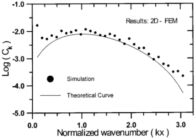
In Fig. 5, we present the results obtained from the sim-ulation (actually, log10 of the results) as a function of k,

and the theoretical curvelog10ck. We observe an excellent

agreement, except for values of k near zero (very long wave-lengths). In this region, there is some deviation from the thermal equilibrium. Presumably, this is due to the fact that modes with longer wavelengths are less susceptible to atten-uation, and for this reason, they do not reach the equilibrium as fast as modes with smaller wavelengths. Besides, we note that in the simulation the time average is taken over a finite time interval, differently of what occurs in theory.

Figure 5. The theoretical spectral distribution of the electric field energy (solid curve) compared to the 1D PIC-FEM simulation (dots).

In the 2D simulations, we also considered periodic boundary conditions with immobile ions as a charge neu-tralizing background. Equally, in this case, electrons that leave from the sides of the rectangular grid are placed in the other side. We used a grid of 64 points in the x-direction and 128 points in the y-direction. We usedN = 294,916 parti-cles, grid spacings∆x= ∆y =λDe, thermal velocities of

vt=λDeωpein both directions,∆t= 0.2ω−pe1, and we run

the code until325ω−1

In the PIC-FEM code, we used linear interpolation func-tions in the x and y direcfunc-tions. In this case, the expression from the electric field average energy of the fluctuations de-pends onkxandkyand is given by

c(kx, ky) =

(E2

x(kx, ky) + (Ey2(kx, ky))N

(v2

tx+vty2)

=

Ã

1 + 4(sin

2₍kx

2) +sin2(

ky

2))2λ2De

(sin2_(k

x) +sin2(ky))W12(kx)W22(ky)

!−1

(35)

whereW1(k) =W2(k) = (sin (k/2)/(k/2))2.

In the simulation we used a constant value forky

(nor-malized) equal to 2π(61/128), a value arbitrarily chosen among the possible values ofky.

In Fig. 6, we present the results of the PIC-FEM code for the 2D simulations adopting a constantky. There is a

good agreement with the theoretical results. The same ob-servations made in the 1D case, for the region of kx near

zero remain valid. We also note greater deviation from the theoretical curve, than in 1D case, fact also observed with Fourier transform particle models [17].

Figure 6. The theoretical spectral distribution of the electric field energy (solid curve) compared to the 2D PIC-FEM simulation (dots).

IV

Summary

In this work, a 1D and 2D electrostatic computational code was developed in order to study problems that involve bounded collisionless plasmas. The code is based on the coupling of two numerical techniques, the FEM and the PIC modelings. The FEM is largely used in engineering and, in this work, it substitutes the FDM, traditionally applied in plasma physics. One of the advantages of the FEM is the handling of arbitrary boundaries, which can be accurately represented by an unstructured mesh. This feature allows the simulation of devices that present a complex geometry. The boundary condition handling advantages were not ex-plored in this work.

The computations were done considering a plasma in thermal equilibrium and periodic boundary conditions in a rectangular domain, i.e., the plasma is in an open domain.

The computer model is tested by calculating the fluctua-tion spectrum of plasma in equilibrium. To make this com-parison, we developed also a theoretical expression for the fluctuation spectrum of plasmas of finite-size macroscopic particles. We obtained an excellent agreement between the results of our simulations and the expressions developed.

Acknowledgements

This work was supported by FAPESP (grant n. 99/12468-8). The authors acknowledge Dr. V. Decyk for fruitful discussions.

References

[1] J.M. Dawson and A.T. Lin,Particle Simulation, Handbook of Plasma Physics - V.2 -(Elsevier Science Publishers 1984)

[2] J.M. Dawson, Rev. of Mod. Phys.55, 2 (1983)

[3] R. Hockney and J. Eastwood, Computer Simulation Using Particles(McGraw-Hill, New York, 1981).

[4] T. Tajima, Computational Plasma Physics: With Applica-tions to Fusion and Astrophysics. (Addison-Wesley Publish-ing Company, 1989)

[5] W.L. Kruer,The Physics of Laser Plasma Interactions, (Addison-Wesley Publishing Company, 1988)

[6] C.K. Birdsall and A.B. Langdon,Plasma Physics via Com-puter Simulation(McGraw-Hill, New York, 1985)

[7] O.C. Zienkiewicz and R.L. Taylor, The Finite Element Method, 4th edition, V.1 and 2(McGraw-Hill, London)

[8] P.P. Silvester and R.L. Ferrari,Finite Elements for Electrical Engineers, 2th edition (Cambridge University Press, 1990)

[9] G. Arfken, Mathematical Methods for Physicists, 2nd edi-tion, (Academic Press, 1970)

[10] O. Axelsson,Iterative Solution Methods(Cambridge Univer-sity Press, 1996)

[11] N.A. Krall and A.W. Trivelpiece, Principles of Plasma Physics(McGraw-Hill 1973)

[12] R. Huber, F. Tauser, A. Brodschelm, M. Bichler, G. Abstre-iter, and A. Leitenstorfer, Nature,414, 286 (2001)

[13] H. Haug, Nature,414, 261 (2001)

[14] N. Rostoker, Nucl. Fus.1, 101 (1961)

[15] V.K. Decyk, Comp. Phys. Rep.4, 245 (1986)

[16] V.K. Decyk, F.S. Tsung, P.C. Liewer, P.M. Lyster, and R.D. Ferraro,“Particle Simulation on Distributed Memory Parallel Computers”, IPFR-UCLA Technical Report, PPG-1446, July 1992.