Bol. Ciênc. Geod. vol.23 número4

(1)

Article

APPLICATION OF AERIAL AND ORBITAL SENSOR PHOTOGRAPHS

TO IDENTIFY AND DELINEATE WATER BODIES

Aplicação de fotografias aéreas e sensores orbitais na identificação e

delineamento de corpos d’água

Luciana Escalante Pereira1,2

Giancarlo Lastoria2

Bruna Semler de Almeida2

Marcelo Haupenthal2

José Marcato Júnior2

Edward Limin Lo3

Antonio Conceição Paranhos Filho2

1_{Universidade Federal de Mato Grosso do Sul (UFMS). Campus do Pantanal (CPAN). Corumbá, MS,}

Brasil. l.escalante.pereira@gmail.com

2 _{Universidade Federal de Mato Grosso do Sul (UFMS). Faculdade de Engenharias, Arquitetura e}

Urbanismo e Geografia (FAENG). Campo Grande, MS, Brasil. g.lastoria@ufms.br, semler.bru@gmail.com, haupen@gmail.com, jrmarcato@gmail.com, antonio.paranhos@pq.cnpq.br

3_{University of Kentucky. Department of Earth and Environmental Sciences. Lexington, KY, USA.}

edward.lo@uky.edu

Abstract:

The application of orbital sensors to identify and delineate water bodies was evaluated in this study. Reference aerial photos were used to measure the surface area of three water bodies in São Gabriel do Oeste, MS, Brazil and assess seven sensors commonly used in environmental studies: ALOS-AVNIR, CBERS 2B-CCD, CBERS 2B-HRC, IRS P6-LISS3, LANDSAT-TM, LANDSAT-ETM+, and LANDSAT-OLI. The images were analyzed with the near infrared (NIR) band, and digital processing techniques including image fusion (spatial enhancement), false-color composition, and pre-processed radiometric correction were applied to some sensors. Image fusion and radiometric correction were applied to three sensors; only color composition was not conducted on the HRC sensor. In all water bodies analyzed, images from the CCD sensor showed the greatest values of imprecision, reaching 192% for Water Body #3 without digital processing. Considering the spectral properties of the NIR band, we expected more precise data from the analyses using this spectral range. However, color composite analyses obtained greater percent precision compared with analyses that only used the NIR band.

(2)

Resumo:

A aplicação dos sensores remotos orbitais para identificação e delineamento de corpos d’água foi avaliado neste estudo. Para isto, foram utilizadas fotos aéreas como referência para obtenção de área de três corpos d’água em São Gabriel do Oeste, MS- Brasil, sendo analisados sete sensores comumente aplicados em estudos ambientais: ALOS-AVNIR; CBERS CCD; CBERS 2B-HRC; IRS P6-LISS3; LANDSAT-TM; LANDSAT-ETM+ e LANDSAT-OLI. As imagens foram analisadas com a banda do Infravermelho Próximo, além disso, técnicas de processamento digital foram aplicadas em alguns sensores. As técnicas de processamento digital utilizadas foram à fusão de imagens, a composição falsa-cor e a correção radiométrica (pré-processamento), sendo a fusão e a correção radiométrica aplicadas em três sensores. A composição colorida só não foi realizada no sensor HRC. Dos corpos d’água analisados, as imagens do sensor CCD foram as que apresentaram maior valor de imprecisão, chegando a um valor de 192% para o corpo d’água #3 na imagem CCD sem processamento digital. Considerando as propriedades da banda espectral infravermelho próximo, esperavam-se dados mais precisos das análises feitas com a mesma. Entretanto, as análises feitas em composição colorida obtiveram melhores percentuais de precisão do que as analisadas somente com a banda do infravermelho próximo.

Palavras-chave: Geotecnologia; Imagens aéreas; Sensoriamento remoto.

1. Introduction

Within the broad framework of geotechnology, remote sensing has been accomplished since the 19th century through acquisition of aerial photos. Although the earliest form of remote sensing technology, aerial photography is still an important source of data because of its high spatial resolution and flexible coverage (Schowengerdt 2007).

The resources available from remote sensing has constantly improved from the first photos taken from balloons to the advancement of satellite-acquired images.

With the advances in remote sensing and the availability of free online data, each day sees increasingly more new users, which requires a better understanding of the potential applications of each product.

Remote Sensing (RS) as a science consists of data or image acquisition of an object that is distant from the sampling sensor (Campbell 2002), including digital and analog aerial photos in addition to satellite and radar images (Paranhos Filho, Torres and Lastoria 2008). RS is fundamentally based on measuring the interaction between electromagnetic radiation and the desired targets (Bielenki Júnior and Barbassa 2012). The radiation that best distinguishes water bodies is concentrated in the near infrared (NIR) region.

According to Figueiredo (2005), each target exhibits a spectral behavior as a function of the interaction with the incident electromagnetic radiation (ER). Even for targets with a known spectral behavior, the signal is not unique or permanent because a single object may present differences due to the characteristics of the sensor. In addition, water reflectance is affected by different factors such as total suspended sediment, chlorophyll concentration and angle of incident radiation, etc.

(3)

the specifications of each sensor such as spatial resolution, spectral resolution and radiometric resolution. Image processing techniques were performed on several sensors to measure their effect on sensor outputs.

The use of aerial photos to measure the results of satellite images shows aspects such as format standards and object surroundings that are not always detectable in satellite images.

Given this scenario, the objective of the present study was to evaluate the use and capability of distinguishing different orbital sensors in the identification and delineation of water bodies.

2. Materials and Methods

2.1 Study Area

The water bodies in this study (Figure 1) vary in size and are located in the municipality of São Gabriel do Oeste (19º23'43" S, 54º33'59" W) in the state of Mato Grosso do Sul, Brazil. The municipality belongs to the sub-watersheds of the Aquidauana and Taquari rivers and is found within the Upper Paraguay River Watershed (BAP, in Portuguese).

Figure 1: Spatial distribution of the three water bodies studied. Image acquired with Landsat-8

(4)

Prior to analyses, the water bodies must be visible in all images, so images with 30-m spatial were used to delineate the areas. The study site also had to be suitable to Unmanned Aerial Vehicle (UAV) flyovers.

The sites were selected based on the size and variation of pure water pixels from the water bodies. Three sizes of water bodies were chosen: small (water body #2), medium (water body #3), and large (water body #1). Areas of different size were selected to evaluate how much spatial resolution interferes with objects in the image and to identify other attributes that can limit object visualization.

Because UAV aerial images had high spatial resolution, they were used as a reference when measuring the surface areas occupied by water bodies. The photos were taken on November 17, 2012 and merged and orthorectified using Agisoft PhotoScan software version 1.1 to improve precision (Agisoft LLC 2014).

2.2 Satellite and sensors

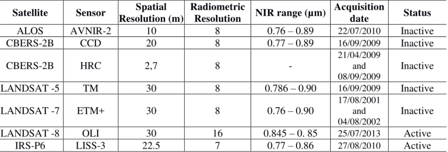
Seven types of sensors that are commonly applied to environmental studies were used: AVNIR (Advanced Visible and Near Infrared Radiometer type 2), CCD (Couple Charged Device), ETM+ (Enhanced Thematic Mapper Plus), HRC (High Resolution Panchromatic Camera), LISS3 (Linear Imaging Self-Scanner), OLI (Operational Land Imager), and TM (Thematic Mapper). Table 1 shows the main features of the sensors.

Table 1: Main features of the sensors used.

Satellite Sensor Spatial

Resolution (m)

Radiometric

Resolution NIR range (µm)

Acquisition

date Status

ALOS AVNIR-2 10 8 0.76 – 0.89 22/07/2010 Inactive

CBERS-2B CCD 20 8 0.77 _– 0.89 16/09/2009 Inactive

CBERS-2B HRC 2,7 8 - 21/04/2009 and

08/09/2009 Inactive

LANDSAT -5 TM 30 8 0.786 – 0.90 16/09/2009 Inactive

LANDSAT -7 ETM+ 30 8 0.76 – 0.90 17/08/2001 and

04/08/2002 Inactive

LANDSAT -8 OLI 30 16 0.845 – 0. 85 25/07/2013 Active

IRS-P6 LISS-3 22.5 7 0.77 – 0.86 27/08/2010 Active

(5)

2.3 Data Analysis

A geographic database was built in the GIS program SPRING version 5.2.4(Camara et al. 1996) to generate and process data. The QGIS (OSGeo 2013) program was used to measure the surface area of the water bodies in the aerial photos. Gimp 2.8 (the GIMP Team, 2013) was used for final image editing such as converting TIFF (Tagged Image File Format) to JPG (Joint Photographic Experts Group) format and standardizing file resolution to 300 dpi. Table 2 exhibits the data acquired by the sensors.

The water bodies were analyzed in the near infrared (NIR) region, which is present in all sensors of this study. It distinguishes well between elements such as vegetation and water. However, since human vision is based on colors, the analytical results of images in false color were also examined. Some image processing techniques were applied to optimize the information obtained with the sensors, including radiometric correction (RC) and spatial enhancement (image fusion).

For some sensors, image radiometric correction was applied to improve the quality of the captured images to match actual conditions as closely as possible. The sensors CCD, HRC of the CBERS-2B satellite (INPE 2011a) and ETM+ of Landsat -7 were radiometrically corrected. In the case of the ETM+ sensor, images from the INPE (2011b) database were used.

From the radiometric correction tools available in SPRING, restoration and filtering were applied. Restoration helps correct image distortions introduced by the optical sensor during image production, and filtering is a pixel-by-pixel image transformation based on the gray shade of each pixel and the gray shades of its neighboring pixels(INPE 2006).

Spatial enhancement, also known as image fusion, was applied to images from the ETM+ and OLI sensors (30-m spatial resolution) to improve resolution. The main method used was the HSI-RGB (H=hue, S=saturation, I=intensity) transformation where the panchromatic channel replaces the intensity channel. This conversion produces a final image with a 15-m spatial resolution.

Spatial resolution is one the key variables determining whether an object can be observed in the image. Water bodies were delineated by visual interpretation, so contrast enhancement was applied to better distinguish objects in the scene. To minimize subjective interpretation, one person delineated all water bodies.

3. Results and Discussion

As mentioned, contrast enhancement was applied to the images for visual interpretation, which improves visual quality in the scene. According to Ponzoni, Shimabukuro and Kuplish (2012),

“the visual identification of objects in images captured by remote sensors is effective when geometric characteristics and general appearance of the objects are of interest.” Since every region

is unique, the results of each water body are presented separately.

(6)

between the object limits in each scene. The actual offset between the borders of two targets may

be larger than the sensor’s spatial resolution, which is one of the basic factors in selecting a satellite.

With visual interpretation, the human operator is responsible for identifying these limits to identify and analyze the characteristics of each sensor. Measuring the surface area of water bodies in different sensors helps us understand and better identify the characteristics of each sensor. By using the NIR band, we expected that the limits of water bodies and their surroundings would be easier to identify, except in wetlands where pixel mixing is common between two classes (water and wetland). The advantage of using NIR to delineate water bodies is easy identification for visual interpretation, where the distinction among various gray shades was better than in RGB (Red-Green-Blue) composition.

This effect occurred because color composition causes more confusion when defining border limits. Pixel mixing was less perceived in NIR than in false color composition, which minimized uncertainty compared with defining pixel limits by naked eye.

In the NIR band, higher reflectance values are expected for vegetation. When the rate of photosynthesis is higher, the region appears clearer, which generates good contrast with water that often appears in darker hues.

The use of digital processing techniques including color composition, image fusion, and radiometric correction helps further the understanding and discussion of potential differences that a particular sensor can create in visual interpretation.

The imprecision of each sensor was estimated by calculating the difference between the surface area measured in the image acquired by the sensor and in the reference aerial image.

3.1 Water Body #1

The first water body is linked to an affluent of the Coxim River. It was the largest water body analyzed, and according to estimates from images acquired by UAV (16-cm spatial resolution), it occupied a surface area of 41,112 m². It has low vegetation and sparse shrubs on its margins (Figure 2).

Figure 2: Orthorectified aerial photo of water body #1, obtained by unmanned aerial vehicle (UAV). This image was used as reference for surface area and site identification. Acquisition

(7)

The high spatial resolution of the HRC sensor helped produce satisfactory results. Moreover, the features of this sensor are enhanced by radiometric correction, further improving its precision. As a result, the surface area estimated by HRC images with radiometric correction is the closest to the area visually determined from the reference aerial image. The values are show in Table 2.

Table 2: Measurement of the surface area of water body #1 and percent imprecision of each

analyzed sensor. RC (Radiometric Correction) and IF (Image Fusion)

Aerial Orthophoto = 41,112m2 Monochromatic

photo interpretation

Imprecision (%)

False Color Composite

Sensor Area (m²) Area (m²)

ETM+ 37,275 9.33 42.780 4.06

ETM+/IF 45,782 11.36 45.686 11.13

ETM/RC 43,344 5.43 42.470 3.30

TM 48,681 18.41 45.167 9.86

CCD 72,681 76.79 62.638 52.36

CCD/RC 38,942 5.28 42.941 4.45

HRC 39,126 4.83 - -

HRC/RC 40,795 0.77 - -

AVNIR-2 47,968 16.67 46.384 12.82

LISS-3 49,640 20.47 40.427 1.67

OLI 53,407 29.91 49.739 20.98

OLI/IF 35,737 13.07 45.107 9.72

CCD was the least precise sensor, reaching imprecision rates above 76% in the analysis of monochromatic photos. However, as observed for HRC, radiometric correction improved the features of CCD images, significantly reducing the imprecision of monochromatic photos to 5.28%. The LISS-3 sensor surpassed other sensors and may have a wider application in environmental studies. The outputs of the sensors are shown in Figure 3.

Figure 3: Graphical representation of data. Images obtained with the HRC sensor were used in

monochromatic analysis. Monochromatic photo interpretation shows the higher precision of CCD images with radiometric correction and lower precision of non-treated CCD images. In true

color composite, the LISS-3 sensor is exceptional with imprecision of only 1.67%.

The interaction between the electromagnetic radiation and the target objectdepends on the object’s

(8)

appear differently. This effect was observed in CCD and TM images analyzed in the NIR region. The radiometric correction on the ETM+ sensor gives the image an oversaturated appearance. A set of weirs near water body #1 could be distinguished in the aerial photos and in most sensor images. In the CCD image, the wiers appear connected to the reservoir, without barriers between them. Sensor imprecision is reduced in true color composition, but it remains high for CCD (52%) and OLI (nearly 21%).

3.2 Water Body #2

The smallest analyzed area was located near highway BR-163 and the municipality, in a region lacking wetlands and with low vegetation around the water body (Figure 4). Pixel mixture in this area was less frequent than in the other water bodies of the study.

Figure 4: Orthorectified aerial photograph of water body #2, obtained by UAV. The image was

used as reference for surface area and site identification. Acquisition date: November 17, 2012. Spatial resolution: 10 cm.

(9)

ETM+ 5,667 58.69 3.258 8.76

ETM+/IF 3,832 7.31 3.245 9.13

ETM/RC 4,552 27.47 4.552 27.47

TM 5,434 52.17 3.599 0.78

CCD 4,037 13.05 4.432 24.11

CCD/RC 5,197 45.53 4.348 21.76

HRC 4,320 20.97 - -

HRC/RC 3,359 5.94 - -

AVNIR-2 3,246 9.10 3.246 9.10

LISS-3 4,036 13.02 2.844 20.36

OLI 3,591 0.56 3.591 0.56

OLI/IF 2,680 24.95 3.553 0.50

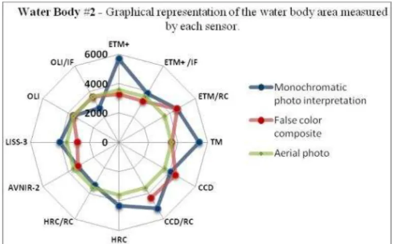
Image processing techniques, especially spatial enhancement, improved ETM+ outputs. Because of the features of each sensor, the same technique can produce different effects. Spatial enhancement, for instance, reduced water body surface area in the NIR range of the OLI sensor. Figure 5 compares and contrasts the sensor results.

Figure 5: Graphical representation of data. Data spatialization allows for rapid interpretation,

indicating the sensor with higher and lower precision based on the reference measurement. It also shows disparities among the outputs. The combination of spectral bands improved the performance of the TM sensor, which was more accurate than the aerial orthophoto in false color

composite.

(10)

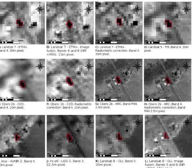
Figure 6: Images of water body #2 analyzed in the near infrared (NIR) region. In this band, water bodies absorb a great amount of energy, becoming darker and facilitating demarcation. The HRC sensor covers the visible and NIR bands. Water body #2 represents an area where the pixels of

the water body are different from its surroundings, making visual interpretation clearer since pixels are not mixed. The technical fusion in the OLI images shows more detailed elements, with

roofs and roads exhibiting similar spectral responses.

The OLI sensor has not only a higher radiometric resolution but also higher spectral resolution. This occurs because it has more spectral bands and the narrowest infrared range. Combined with spectral enhancement, it is a free tool with many potential uses, especially in construction areas. Spatial resolution is one of the key characteristics that determine which elements are detected in an image. However, spatial resolution alone does not improve data precision for the sensor. With 30-m spatial resolution, OLI was the best sensor in monochromatic analysis and was equally precise in color analysis without image processing.

3.3 Water Body #3

(11)

ETM+ 28,425 130.46 20.357 65.05

ETM+/IF 16,258 31.81 20.706 67.88

ETM/RC 15,290 23.97 18.968 53.79

TM 25,203 104.34 20.267 64.32

CCD 36,052 192.30 27.668 124.32

CCD/RC 20,737 68.13 21.172 71.65

HRC 13,761 9.14 - -

HRC/RC 12,369 0.28 - -

AVNIR-2 24,358 97.49 24.358 97.49

LISS-3 21,225 72.08 16.581 34.43

OLI 23,447 90.10 21.639 75.44

OLI/IF 10,789 12.53 14.391 16.68

Fused OLI images presented the best results of the color composite images, and also had good precision in monochromatic analysis. The HRC sensor with radiometric correction had the best overall output, measuring an estimated dam surface area of 12,369 m². Figure 7 shows a graphical data plot for water body #3.

Figure 7: Graphical representation of data. Surface area estimates varied among the sensors, and

both monochromatic and false color analyses had high rates of imprecision.

Given that the infrared band is very sensitive to moisture, the combined reflectance and pixel mixture are likely higher when areas surrounding the water bodiesare wet or saturated, as observed in water body #3. The phenomenon of pixel mixture, which is the occurrence of more than one classwithin a resolution cell (pixel) (Caimi 1993), often occurs in images from sensors with lower spatial resolution.

(12)

Figure 8: Orthorectified aerial photography of water body #3, obtained by UAV. The image was

used as reference for surface area and site identification. Acquisition date: November 17, 2012. Spatial resolution: 16 cm.

Despite the differences in each sensor’s measurement techniques, water body #3 did not present major difficulties for visual interpretation. The contrast between water and vegetation helped with delimitation.

As observed for water body #1, radiometric correction of the CCD sensor improved the quality of the information obtained, enhancing differentiation among the objects. An unprocessed CCD image, however, exhibited the worst result of all sensors in this study. As such, the CCD sensor in the NIR band was the least precise sensor for modeling water bodies.

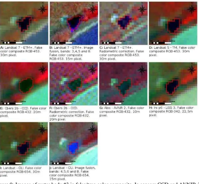
In the color composite sensor images in Figure 9, the difference in the delimited area between the original CCD image (Figure 9-E) and the other images can be compared.

AVNIR 2 has good spatial resolution (10 m), but failed to provide a satisfactory delimitation of the water bodies. Sensors with lower spatial resolution, such as LISS3, for instance, provided better results.

Of the 3 areas analyzed, the outputs were most consistent for water body #2, which showed low spectral confusion. Radiometric correction performed satisfactorily by decreasing sensor imprecision in most situations.

(13)

Figure 9: Images of water body #3 in false/true color composite. In sensors CCD and AVNIR-2, the RGB channels were associated to red, green and NIR bands. In Landsat series sensors and LISS-3, true color composite was based on NIR, SWIR and red bands. The study focused on the

accuracy of surface area measurements, but the patterns of water body shape in each image was noteworthy. The different shapes are related to the spectral bands used and the unique response

of each sensor to the different targets.

4. Final Considerations

(14)

The other sensors have large databases available, with more than 30 years of data collection by the Landsat series. In addition, the results presented here can support other studies based on new sensors that are launched.

The CCD sensor produced the most imprecise data, so radiometric correction was fundamental to improve image quality.

LISS-3 is another sensor with good image quality, and its data could be further explored. Despite the low radiometric resolution and moderate spatial resolution (22.5 m), its images allow for good visual analysis. The LISS-3 sensor is also coupled with the active ResourceSat-2 satellite, which provides free images and could be further explored in Brazil.

In this study, only one commercial sensor (AVNIR-2) was used. However, the results obtained corroborated that free data are becoming stronger in the geotechnology field because of their excellent quality.

ACKNOWLEDGEMENTS

The Coordination for the Improvement of Higher Education Personnel (CAPES) awarded Luciana Escalante Pereira with a MSc fellowship. The National Council for Scientific and Technological Development (CNPq) also funded an ACPF PQ fellowship (process 305300/2012-1).

REFERENCES

Agisoft (2014). Software Agisoft PhotoScan. Avaliable

at: <http://www.agisoft.ru/products/photoscan/professional/buy/educational/> [Accessed 20 January 2014]

Bielenki Júnior, C. Barbassa, A. P. 2012. Geoprocessamento e Recursos Hídricos: aplicações práticas. São Carlos: EdUFSCAR.

Caimi, D. 1993. O problema do pixel de mistura: um estudo comparativo. Porto Alegre. 104p. Dissertação (Mestre em Sensoriamento Remoto). Centro Estadual de Pesquisas em Sensoriamento Remoto. Universidade Federal Do Rio Grande Do Sul. Available at: <http://www.lume.ufrgs.br/handle/10183/1373> [Accessed 21 July 2013]

Camara, G. Souza, R. C. M. Freitas, U. M. Garrido, J. 1996. SPRING: Integrating remote sensing and GIS by object-oriented data modelling. Computers & Graphics, 20(3), pp.395-403.

Campbell, J. B. 2002. Introduction to remote sensing. 3rd ed. CRC Press.

Figueiredo, D. 2005. Conceitos Básicos de Sensoriamento Remoto. Available at:

<http://www.conab.gov.br/conabweb/download/SIGABRASIL/manuais/conceitos_sm.pdf> [Accessed 19 August 2013].

Global Land Cover Facility – GLCF. n.d. LANDSAT 7 ETM Canais 3, 4, 5 e 8. University of Maryland. Earth Science Data Interface. Órbita 225 ponto 073. Available at: <http://glcfapp.glcf.umd.edu:8080/esdi/> [Accessed 05 May 2012].

(15)

Instituto Nacional de Pesquisas Espaciais - INPE. 2011a. CBERS-2B/ CCD Banda 4. São José dos Campos Imagem de Satélite. Órbita 163 ponto 122. Available at: <http://www.dgi.inpe.br/CDSR/> [Accessed 10 July 2012].

Instituto Nacional de Pesquisas Espaciais - INPE. 2011b. CBERS-2B/ HRC Bandas 1. São José dos Campos Imagem de Satélite. Órbita 163_A ponto 121. Available at: <http://www.dgi.inpe.br/CDSR/> [Accessed 16 August 2012].

Instituto Nacional de Pesquisas Espaciais – INPE. 2011b. LANDSAT 7 ETM Canal 5. São José dos Campos. Imagem de Satélite. Órbita 225 ponto 073. Available at: <http://www.dgi.inpe.br/CDSR/> [Accessed 09 November 2012].

Instituto Nacional de Pesquisas Espaciais – INPE. 2006. SPRING – Sistema de Processamento de Informações Georreferenciadas. Manuais: Tutorial de Geoprocessamento – Restauração e Filtragem. Available at: <http://www.dpi.inpe.br/spring/portugues/tutorial/index.html> [Accessed 07 January 2014].

OSGeo. Open Source Geospatial Foundation. QGIS. 2013. Open Source Geographic Information

System (GIS). Version 2.0.1. “Dufour”. Available at: <http://qgis.org/> [Accessed 26 July 2012]. Paranhos Filho, A. C. Torres, T. G. Lastoria, G. 2008. Sensoriamento Remoto Ambiental Aplicado: Introdução as Geotecnologias. 1st ed. Campo Grande – MS. Editora UFMS.

Ponzoni, F. J. Shimabukuro, Y. E. Kuplich, T. M. 2012. Sensoriamento Remoto da Vegetação.

2nd ed. São Paulo – SP. Editora Oficina de Textos. Atualizada e ampliada.

Schowengerdt, Robert. A. 2007. Remote sensing: Models and methods for image processing. 3rd

ed.

United States Geological Survey, 2012. Landsat Missions [online]. Available at: <http://landsat.usgs.gov/> [Accessed 07 September 2013].