Article
ANALYSIS OF ISOSTATICALLY-BALANCED CORTICAL MODELS
USING MODERN GLOBAL GEOPOTENTIAL MODELS
Análise de modelos córticos isostaticamente equilibrados utilizando modelos
geopotenciais globais modernos
Claudia Infante1
Claudia Tocho 2,3
Daniel Del Cogliano 2,4
1 Universidad Nacional de Santiago del Estero. Facultad de Ciencias Exactas y Tecnologías. Av. Belgrano (S) 1912. (4200) - Santiago del Estero - Argentina. E-mail: [email protected]//[email protected]
2 Universidad Nacional de La Plata. Facultad de Ciencias Astronómicas y Geofísicas. Paseo del Bosque s/n, La Plata, Argentina. E-mail: [email protected] /[email protected]
3 Comisión de Investigaciones Científicas de la Provincia de Buenos Aires. Calle 526 e/10 y 11. La Plata, Buenos Aires. Argentina.
4 Consejo Nacional de Investigaciones Científicas y Técnicas (CONICET). Argentina.
Abstract:
The knowledge of the Earth's gravity field and its temporal variations is the main goal of the dedicated gravity field missions CHAMP, GRACE and GOCE. Since then, several global geopotential models (GGMs) have been released. This paper uses geoid heights derived from global geopotential models to analyze the cortical features of the Tandilia structure which is assumed to be in isostatic equilibrium. The geoid heights are suitably filtered so that the structure becomes apparent as a residual geoid height. Assuming that the geological structure is in isostatic equilibrium, the residual geoid height can be assimilated and compared to the isostatic geoid height generated from an isostatically compensated crust. The residual geoid height was obtained from the EGM2008 and the EIGEN-6C4 global geopotential models, respectively. The isostatic geoid was computed using the cortical parameters from the global crustal models GEMMA and CRUST 1.0 and from local parameters determined in the area under study. The obtained results make it clear that the isostatic geoid height might become appropriate to validate crustal models if the structures analyzed show evidence of being in isostatic equilibrium.
Keywords: Geopotential models, crustal models, isostatic geoid, EGM2008, EIGEN-6C4,
GEMMA, CRUST1.0
Resumo:
modelos geopotenciais globais (GGMs) foram lançados. Este artigo usa os níveis de geoide derivados de modelos geopotenciais globais para analisar as características corticais da estrutura de Tandilia, que se supõe estar no equilíbrio isostático. As alturas do geoide são adequadamente filtradas para que a estrutura se torne aparente como uma altura residual de geoide. Supondo que a estrutura geológica esteja em equilíbrio isostático, a altura residual do geoide pode ser assimilada e comparada com a altura do geoostato isostático gerada a partir de uma crosta compensada isostática. A altura residual de geoide foi obtida a partir dos modelos geopotenciais globais EGM2008 e EIGEN-6C4, respectivamente. O geóide isostático foi calculado utilizando os parâmetros corticais dos modelos crustais globais GEMMA e CRUST 1.0 e dos parâmetros locais determinados na área estudada. Os resultados obtidos deixam claro que a altura do geoide isostático pode se tornar apropriada para validar modelos crustais se as estruturas analisadas mostrarem evidências de estar em equilíbrio isostático.
Palavras-chave: Modelos geopotenciais, modelos crustais, geoide isostático, EGM2008,
EIGEN-6C4, GEMMA, CRUST1.0.
1. Introduction
The isostatic analysis of geological structures was traditionally made with isostatic gravity anomalies. However, the information provided by the geoid heights anomalies (Fowler 2005, pp 214) may be used to complement and/or validate these studies (Del Cogliano 2006; Crovetto, Molinari and Introcaso 2006; Cornaglia 2007).
Anomalous masses on the terrestrial crust disturb and undulate the geoid equipotential surface of the Earth's gravity field. The geoid height anomalies resulted by an isostatic density distribution can be compared to those geoid height anomalies seen on the actual structure if the wavelengths are compatible (Fowler 2005). The result presented in this paper constitutes another way to analyze isostasy (Haxby and Turcotte, 1978; Crovetto, Molinari and Introcaso 2006).
This study examines a profile over Tandilia structure located in Buenos Aires province, Argentina. By comparing the observed geoid anomaly, appropriately filtered in the area under study, with a perfectly compensated cortical model, it will be possible to draw a conclusion about the crust features (Del Cogliano 2006). This is feasible today because the resolution of the heights of the
Earth’s geoid has improved considerably during the past years through the dedicated gravimetry
satellite missions like CHAMP (Challenging Minisatellite Payload), (Reigber et al. 2002); GRACE (Gravity Recovery and Climate Experiment) (Tapley, Bettadpur, Watkings and Reigber 2004) and the GOCE (Gravity Field and Steady State Ocean Circulation Explorer), (Drinkwater et al., 2003).
2. Isostatic geoid height anomaly
The actual Earth´s gravitational potential Vactual can be expressed as the sum of the gravitational
potential produced by the isostatic regularized Earth Vreg, and an isostatic disturbing potential Tisost
resulting from the topography and the corresponding isostatic compensating model (Del Cogliano 2006):. It is possible to express it as (equation 1):
actual reg isost I
V V T v
(1)
where vI represents the deviation from the isostatic model and the errors made in its evaluation.
Rearranging equation (1), results (equation 2):
isost actual reg I
T V V v
(2)
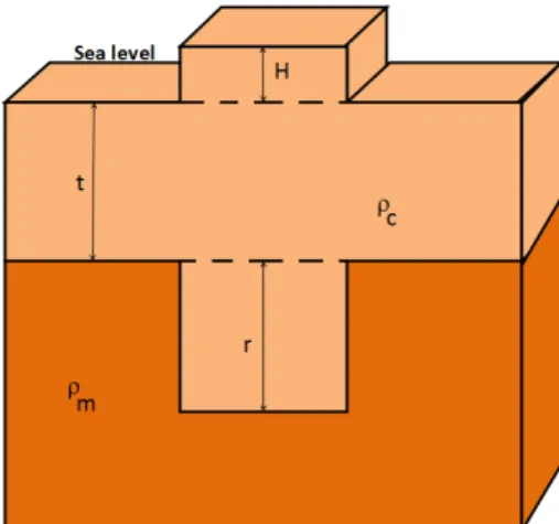
When considering the Airy’s compensating model (Fowler 2005), (Figure 1), a reference structure having a normal crust of thickness t, crust density c, mantle density m and height H will be isostatically compensated by the existence of a root of thickness r so that (equation 3):
c
m c
H
r
(3)
Figure 1: Airy isostatic compensation model.
It can be shown that the disturbing isostatic potential, Tisost, produced by the topographic mass of
a height H and root r will be, according to Fowler (2005), as follows (equation 4):
2
c
isost c
m c
T G H t H
(4)
where G is the universal gravitational constant; c and m are the crust and top mantle density, respectively; t is the thickness of the crust of reference and H is the structure´s height.
By applying the Bruns’ formula (Heiskanen and Moritz 1967, pp 85) that relates geoid height Nisost
isost isost
T N
(5)
where is the normal gravity computed at the computation point using Somigliana’s formula (Heiskanen and Moritz 1967, pp 70). Then:
2 c c isost m c G H
N t H
(6)
Equation (6) solves geoid height anomaly Nisost, resulting from an isostatic density anomaly, for a
compensated structure under Airy’s hypothesis in terms of a function depending just upon the
height of the structure under study, the values for the cortical and mantle densities and a reference crust isostasy (Haxby and Turcotte 1978; Fowler 2005).
3. Methodology for an isostatic analysis of geological structures
To analyse the cortical features of a geological structure, the observed and appropriately filtered geoid height is compared to the corresponding geoid for a perfectly compensated cortical model. For that reason, the observed geoid height must first be filtered in order to keep the signals related to the structure under study. This residual geoid height thus estimated is then compared to the geoid height anomaly calculated from the isostatically balanced model. The differences among them will show the fit of the adopted reference model and the real one.
The observed geoid height is taken from a global geopotential model (Nmod) and it can be written as the sum of a regional component (Nregional) that reflects the predominating behavior in the study area and a residual component (Nresidual), related to the local structure analyzed(Del Cogliano 2006). It will be expressed as (equation 7)
mod regional resisual n
N N N v (7)
where n stands for the errors of the global geopotential model. Thus, one can write (equation 8):
mod
residual regional n
N N N (8)
If the residual component is related to the discrepancies between the actual and the regularized crusts, the residual and the isostatic undulations can be assimilated (Equation 9).
The isostatic geoid height anomaly Nisost, is calculated using equation (6) with the crustal
parameters of the adopted reference model.
Then, if isostatic equilibrium exists (equation 9):
residual n isost I
N v N v (9)
where I represents the deviations from the isostatic model and the errors made in its evaluation.
I res N isost
Once the isostatic component has been eliminated from the residual geoid undulation, according to equation (10), the values for Ishow the eventual discrepancy of the analyzed structure from the isostatic model adopted.
4. Study area
For this paper, the Tandilia system, located southwest of Buenos Aires province, Argentina, has been chosen. The topographic structure under study is almost 60 km wide, extending along approximately 350 km in linear development with an imaginary NorthWest- SouthWest axis. The analysis is presented on a 220-km-long profile with an azimuth of 129 degrees (Figure 2).
Figure 2: Tandilia Hill profile location on a topographic map. Scale units are measured in meters.
4.1 Geological features of the structure
The Tandilia structure is located in the Rio de la Plata craton extending from Uruguay in the north
to the Tandilia region in the south (Figure 3). The craton’s thicknesses typically vary between 40
with SW Africa and an early bonding of these cratonic cores along the development of SW Gondwana (Dalla Salda 1979; Dalla Salda 1982; Del Cogliano 2006).
The thickness of the cratons typically varies between 40 and 45 km. In Namibia, a portion of Africa belonging to the Kalahari craton, the cortical thickness ranges from 41 to 48 km. In central Brazil, recent determinations yield values greater than 40 km (Del Cogliano 2006, pp86).
The CRUST 5.1 model (Mooney, Laske and Masters 1998), in its 2º x 2º version, tentatively suggests bark thicknesses of the same order. Due to the lack of seismologic data related to Tandilia, crust values are interpolated from the global crust model CRUST 1.0 (Laske, Ma, Masters and Pasyanos 2013) towards the South - East area, between continental and oceanic margin. The consequence is that the thicknesses that it throws punctually in the studied area are somewhat smaller than the previous ones.
Figure 3: Geological map of Tandilia (Dalla Salda, Barrio, Echebeste and Fernandez 2005;
extracted from Del Cogliano 2006)
Tandilia structure has a length of 350 km and a wide less than 60 km. It could be expected that small structures like this could not produce roots according to the Airy isostatic model due to the high rigidity of the crust (Introcaso 1997, pp. 297).
However, the geological processes that explain the origin of the present Tandilia structure formation are related to mountains with more than 8 km of height and much more extended than the existing ones. Then, in a metamorphic environment the isostasy had to balance mountains and roots. The subsequent erosion process of the topography had to be accompanied by the corresponding reduction in the roots (Del Cogliano 2006, pp. 85).
5. Data used
5.1 Global geopotential models: EGM2008 and EIGEN-6C4
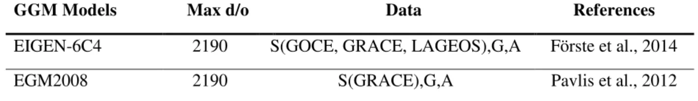
Two global geopotential models, up to their maximum degree and order (d/o), have been used in this study (Table 1). These models were released for public use via the International Centre for Global Earth Models (ICGEM) on http://icgem.gfzpotsdam.de/ICGEM/ICGEM.html. EGM2008 (Pavlis, Holmes, Kenyon and Factor 2012) and EIGEN-6C4 (Förste et al., 2014) are used as the observed geoid.
Table 1: Global Geopotential Models used as observed geoid in this study.
GGM Models Max d/o Data References
EIGEN-6C4 2190 S(GOCE, GRACE, LAGEOS),G,A Förste et al., 2014
EGM2008 2190 S(GRACE),G,A Pavlis et al., 2012
Table note: Data: S = Satellite Tracking Data, G = Gravity Data, A = Altimetry Data.- GRACE (Gravity Recovery And Climate Experiment).
GOCE (Gravity field and steady state Ocean Circulation Explorer). LAGEOS (Laser GEOdynamics Satellite)
The ultra-high resolution Earth Gravitational Model 2008 (EGM2008) is available by the National Geospatial-Intelligence Agency (NGA) and the EIGEN-6C4 has been jointly elaborated by GFZ Potsdam and the GRGS /CNES Toulouse. The maximal spatial resolution of both models is approximately of 9 km.
5.2 Global Crustal Models: GEMMA and CRUST 1.0
To estimate the isostatic geoid height anomaly, the parameters taken as reference were selected from GOCE Exploitation for Moho Modeling and Applications (GEMMA) (Barzaghi et al, 2014) and CRUST 1.0 (Laske, Ma, Masters and Pasyanos 2013).
The main objective of GEMMA project is to improve the knowledge of the crust-mantle discontinuity surface – the Moho – by using data coming from the GOCE satellite mission, ensuring a well distributed and homogeneous global coverage. The Moho depth was derived taking the density contrast (between mantle and crust) as a constant being equal to 0.630 kg/m3 (a homogeneous crust of density 2.67 kg/m3 and a homogeneous mantle of density 3.27 kg/m3 ) (Reguzzoni and Sampietro, 2015). The spatial resolution of the crustal models is 0.5° × 0.5°.
receiver function studies. The receiver function method (RFM) is a commonly used technique to study the crustal and upper mantle velocity structure using temporary and permanent, three-component, short period and broad-band seismic stations (Ryberg and Weber, 2011).
5.3 The local gravimetric geoid model (ESS1175)
The local geoid model ESS1175 (Equivalent Source Solution 1175), (Del Cogliano 2006) was computed using the equivalent source method. It includes 22 GPS/Levelling benchmarks and 1153 gravity anomalies, all of them corresponding to gravity sites interpolated on a grid of 7 km interval.
As result of geological, geophysical and geodetic considerations based on the ESS1175 model, a geological characterization was performed proposing a normal crust of a thickness of 42 km and a density of 2.84 gr/cm3, on a mantle of a density of 3.24 gr/cm3. Hereafter, this crust model will be referred to as ESS1175.
5.4 DTM2006 Digital Terrain Model
The DTM2006.0 (Pavlis, Factor and Holmes 2006) is the digital terrain model used by the ICGEM calculator to obtain the geoid height and Bouguer gravity anomalies in terms of spherical harmonics. The ICGEM calculator allows us to get the topography referred to the EGM2008 geoid. The heights from DTM2006 are used as heights to compute the isostatic geoid height anomaly as was explained in Section 2.
6. Results and discussion
The isostatic geoid height anomaly was estimated by using equation (6) with the cortical parameters determined from the local gravimetric data (ESS1175) (c = 2.84 g/cm3, m = 3.24
g/cm3, t = 42 km) and from both global crustal models: GEMMA (c = 2.85 g/cm3, m = 3.237 g/cm3, t = 35,7 km) and CRUST 1.0 (t = 35.9 km). For the calculation of the isostatic geoid height anomaly with CRUST 1.0, the density values of GEMMA were used, as CRUST 1.0 does not provide density data. The heights were taken from the DTM2006.0 Digital Terrain Model for the three calculations. The statistical summary is shown in Table 2.
Table 2. Statistical summary of the isostatic geoid height anomalies.
Nisost-GEMMA Nisost-CRUST 1.0
Nisost-Local
(ESS1175)
Maximun [m] 2.08 2.07 1.69
Minimun [m] 0.65 0.65 0.65
Range [m] 1.43 1.42 1.04
Average [m] 1.31 1.30 1.16
Standard Deviation [m] 0.29 0.28 0.21
The residual geoid height anomaly (Equation 8) was obtained after subtracting the contribution of the long wavelength of the regional geoid height from the signal of the observed geoid. In this way, the information concerning the Tandilia Hill is kept.
The observed geoid was taken from EGM2008 and secondly, with EIGEN-6C4 global geopotential models, both models up to degree 2190 in terms of spherical harmonics. The regional geoid (Nregional) was computed after the truncation up to degree 36 of the global geopotential model
coefficients. This corresponds to wavelength associated of 1110 km and 550 km of spatial resolution, which is the size of the structure we are trying to analyze. This means that the geological structures higher than 550 km were filtered.
Figure 4: Residual geoid height (units in meters) over the Tandilia structure by using EGM2008
(left) and residual geoid height over the profile by using EGM2008 and EIGEN-6C4 global geopotential models (right).
Figure 4 (left) shows the residual geoid by using EGM2008 model that evidences the Tandilia structure. The effects of the topographic masses generate isolines of the residual geoid that enclose the hills. The spatial distribution of the residual geoid curves of the EIGEN-6C4 model is similar to that of the EGM2008 model; the small discrepancies appearing on the profile differ in a few centimeters as it can be seen in Figure 4 (right). The profile was drawn in the direction of North West to South East. The horizontal axis represents the progressive distance is that direction measured along the profile.
On the same graph, it is seen that the isostatic geoid undulation fits well the residual geoid undulation computed by EGM2008 model. This is shown by the average of the differences that is equal to 0.01 m with a RMS (Root Mean Square) is ± 0.17 m. The range of the differences is close to 1.0 m when using local parameters, while it is 1.4 m when using the GEMMA and CRUST 1.0 parameters (Figure 5).
Figure 5: Differences between residual geoid heights computed with the global geopotential
models EGM2008 and EIGEN-6C4 and the isostatic geoid height anomalies with GEMMA, CRUST 1.0 and ESS1175 crustal parameters.
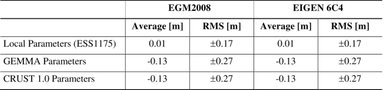
Table 3 shows the statistical summary of the differences between the isostatic geoid height anomalies and the residual geoid heights.
The results obtained show, on one hand, that the parameters used for the theoretical crust model on the Tandilia structure are appropriate, when using the values of the local and global cortical parameters. On the other hand, the goodness of the values of the global cortical models is shown, since in this case the mean of the differences increases only to -0.13 m and RMS is ± 0.27 m. These results further confirm that the structure is in isostatic equilibrium, since they confirm the starting hypothesis (equation 9).
Table 3. Statistical summary of the differences between the isostatic and residual geoid.
EGM2008 EIGEN 6C4
Average [m] RMS [m] Average [m] RMS [m]
Local Parameters (ESS1175) 0.01 0.17 0.01 0.17
GEMMA Parameters -0.13 0.27 -0.13 0.27
CRUST 1.0 Parameters -0.13 0.27 -0.13 0.27
7. Conclusions
It is possible to use the isostatic geoid height anomalies over a geological structure in order to infer its isostatic balance, or vice versa. If the condition of isostatic equilibrium is matched, the cortical features of the geological structure can be validated.
When the cortical model of the structure of Tandilia is analyzed from isostasy hypothesis, the procedure used, allows corroborating the hypothesis.
The results show that the parameters used for the theoretical cortical model are appropriate when using both the values of the local data and the values of the global cortical models even though, the first ones present a better fit. The statistics for the residual geoid yields an average of 0.01 m, with a RMS of ± 0.17 m (Infante, 2013). The significance of this adjustment is analyzed based on the effects made upon the geoid produced by the variation of some cortical parameters.
When the GEMMA and CRUST1.0 models are used, the average of the differences increases up to -0.13 m and the RMS of ± 0.27 m.
The highest differences identified in the profile correspond to a well-defined section of the geological structure. These gravimetric signals might be attributed to the existence of mass density anomalies. This repeats in all the geopotential models utilized and should be analyzed in the future.
These results make it evident that the isostatic geoid height anomaly might be appropriate to validate crustal models provided that the structures analyzed show evidence of being isostatiscally balanced.
Therefore, it is concluded that the methodology presented in this study can be applied as a complement and validation of the traditional method that uses gravity anomalies.
REFERENCES
Amante, C. and Eakins, B.W. 2009. ETOPO1 1 Arc-Minute Global Relief Model: Procedures, Data Sources and Analysis. NOAA Technical Memorandum NESDIS NGDC-24.
Barzaghi, R. et al. 2014. Global to local Moho estimate Estimate based Based on GOCE geopotential Geopotential model Model and local Local gravity Gravity dataData. Proceedings of the VIII Hotine-Marussi Symposium - IAG Symposia, Springer.
Bassin, C.; Laske, G. and Masters, G. 2000. The current limits of resolution for surface wave tomography in North America. EOS Trans AGU, 81 (F897. 2).
Cornaglia, L. 2007. La Sierra de San Luis, su estudio geofísico a partir de las ondulaciones del geoide. Entrega del premio “Ing. Eduardo E. Baglietto”. Anales Academia. Nacional de
Ingeniería Buenos Aires. Tomo III: pp. 75-108.
Crovetto, C.; Molinari, R. and Introcaso, A. 2006. Aproximaciones para el cálculo del geoide isostático. Revista de la Asociación Geológica Argentina. SciELO Issue, 61 (3), pp. :336-346.
Dalla Salda, L. 1982. Nama-La Tinta y el inicio de Gondwana. Acta Geológica Lilloana, 16(1), pp.: 23-28.
Dalla Salda, L. , Bossi, J. , and Cingolani, C. , 1988. The Río de la Plata cratonic region of Southwestern Gondwana. Episodes, 11,4, pp. 263-269.
Dalla Salda, L. 1999. Cratón del Río de la Plata. El basamento granítico-metamórfico de Tandilia y Martín García. Anales Geología Argentina. Subsecretaría de Minería. 29,(4), pp. :97-106. Subsecretaría de Minería.
Dalla Salda, L.; de Barrio, R. E.; Echebeste, H. J.; and Fernández, R. R. 2005. El Basamento de las Sierras de Tandilia. Relatorio del XVI Congreso Geológico Argentino. Cap. III, pp.: 31-50.
Del Cogliano, D. 2006. Modelado del Geoide con GPS y Gravimetría. Caracterización de la estructura geológica de Tandil. Tesis Doctoral. F.C.E.I.y.A – U.N.R. http://hdl.handle.net/10915/60243
Drinkwater, M. et al. 2003. GOCE: ESA’s first Earth Explorer Core mission. Earth Gravity Field from Space – From Sensors to Earth Sciences, vol. 18. Kluwer Academic Publishers, Dordrecht, Netherlands: Kluwer Academic Publishers, pp. 419–432
Fowler, C. M. R. 2005. The solid earth. An introduction to Global Geophysics. - Cambridge University Press. 2 edition -704 p.- ISBN 10: 521 89307 0. ISBN 13: 978-0521893077.
Förste, C. et al. 2014. EIGEN-6C4 The latest combined global gravity field model including GOCE data up to degree and order 2190 of GFZ Potsdam and GRGS Toulouse. GFZ Data Services. http://doi.org/10.5880/icgem.2015.1
Haxby, W. and Turcotte, D. 1978. On isostatic geoid anomalies. Journal Geophysical Journal
Vol. 94. (B4), pp. 3876-3890
Heiskanen, W. and Moritz, H. 1967. Physical Geodesy. W.H. Freeman and Company. San Fransisco and London: Freeman and Company. 364 pág.
ICGEM. 2016. International Centre for Global Earth Models http://icgem.gfzpotsdam.de/ ICGEM/ICGEM.html
Infante, C. 2013. Detección de estructuras geológicas potencialmente en equilibrio isostático a partir del análisis de modelos geopotenciales y anomalías de Bouguer. Tesis de Maestría.
F.C.A.y.G. – U.N.L.P. http://hdl.handle.net/10915/33836.
Introcaso, A. 1997. Gravimetría. UNR Editora Publisher. Rosario. Argentina. 355 pág.
Laske, G. and Masters, G. 1997. A Global Digital Map of Sediment Thickness. EOS Trans AGU, 78 (F483).
Laske, G.; Ma, Z.; Masters, G. and Pasyanos, M. 2013. CRUST 1.0.A New Global Crustal Model at 1x1 Degrees. LLNL.
Mooney, W.D; Laske, G. and Masters, T.G. 1998. CRUST 5.1: A global crustal model at 5°x5°.
Journal of Geophysical Research, 103 (B1), pp.: 727-747.
Pavlis, N.; Factor, J. and Holmes, S. 2006. Terrain-related gravimetric quantities computed for the next EGM. http://earth-info.nga.mil/GandG/wgs84/gravitymod/new_egm/ EGM08_papers/ NPavlis&al_S8_Revised111606.pdf
Ryberg, T. and M. Weber, M. 2000. Receiver function arrays: a reflection seismic approach.
Geophys J Int 141 (1): 1-11. doi: 10.1046/j.1365-246X.2000.00077.x
Ramos, V.; Leguizamón, A.; Kay, S.M. and Teruggi, M. 1990. Evolución tectónica de las Sierras de Tandil (provincia de Buenos Aires). 11º Congreso Geológico Argentino. San Juan. Actas 2, pp. 357-360.
Ramos, V. 1999. Geología Argentina. Evolución tectónica de la Argentina. Buenos Aires. Anales 29 (24), pp. 715-759. Buenos Aires.
Reguzzoni, M. and Sampietro, D. 2015. GEMMA: an earth crustal model based on GOCE satellite data. International Journal of Applied Earth Observation and Geoinformation. doi: 10.1016/j.jag.2014.04.002.
Reigber, C. et al. 2002. A high quality global gravity field model from CHAMP GPS tracking data and accelerometry (EIGEN-1S). Geophysical Research Letters, 29 (14), doi:http://dx.doi.org/10.1029/2002GL015064.
Tapley, B.D.; Bettadpur, S.; Watkins, M. and Reigber, C. 2004. The gravity recovery and climate experiment: mission overview and early results. Geophysical Research Letters, 31(9), L09607, doi:http://dx.doi.org/10.1029/2004GL019920. American Geophysical Union.
Teruggi, M.; Leguizamón, M.A. and Ramos V. 1989. Metamorfitas de bajo grado con afinidades oceánicas en el basamento de Tandil: sus implicaciones geotectónicas, provincia de Buenos Aires.
Asociación Geológica Argentina, Revista 43(3), pp. 366-374.
Received in January 19, 2017.