Artigo
*e-mail: [email protected]
APPLICATION OF GA-PLS AND GA-KPLS CALCULATIONS FOR THE PREDICTION OF THE RETENTION INDICES OF ESSENTIAL OILS
Hadi Noorizadeh* and Abbas Farmany
Department of Chemistry, Ilam Branch, Islamic Azad University, Ilam, Iran Mehrab Noorizadeh
Young Researchers Club, Ilam Branch, Islamic Azad University, Ilam, Iran
Recebido em 10/1/11; aceito em 19/3/11; publicado na web em 10/6/11
Genetic algorithm and partial least square (GA-PLS) and kernel PLS (GA-KPLS) techniques were used to investigate the correlation between retention indices (RI) and descriptors for 117 diverse compounds in essential oils from 5 Pimpinella species gathered from central Turkey which were obtained by gas chromatography and gas chromatography-mass spectrometry. The square correlation coeficient leave-group-out cross validation (LGO-CV) (Q2) between experimental and predicted RI for training set by
GA-PLS and GA-KPLS was 0.940 and 0.963, respectively. This indicates that GA-KPLS can be used as an alternative modeling tool for quantitative structure–retention relationship (QSRR) studies.
Keywords: essential oils; gas chromatography-mass spectrometry; QSRR.
INTRODUCTION
Essential oils also called volatile or ethereal oils are aromatic oily liquids obtained from different plant parts and widely used as food lavours.1 The composition of essential oil has been extensively in-vestigated because of its commercial interest in the fragrance industry (soaps, colognes, perfumes, skin lotion and other cosmetics), in aro-matherapy (relaxant), in cancer treatment, in pharmaceutical prepara-tions for its therapeutic effects as a sedative, spasmolytic, antioxidant, antiviral and antibacterial agent. Recently it has also been employed in food manufacturing as natural lavouring for beverages, ice cream, candy, baked goods and chewing gum.2,3Pimpinella is representing in Turkey by 23 spp. (5 endemic), 2 subspecies, and 2 varieties rep-resenting 27 taxa.4 The most widely known and cultivated Pimpinella species is P. anisum. Pimpinella anisum (Anis) fruits (Aniseed) have been use in Turkish folk medicine as carminative, appetizers, seda-tive, and agents to increase milk secretion.5Aniseed is an important agricultural crop of Turkey. The main volatile compounds found in Pimpinella oils were monoterpenes, sesquiterpenes, trinorsesquiter-penes and phenylpropanoids (propenylphenols,pseudoisoeugenols). These entire compounds have been identiied by gas chromatography and gas chromatography-mass spectrometry (GC–MS).
However, in the case of GC the identiication of chromatographic peaks is just carry out by means of comparison of retention indices with reference compounds. This means that due to the complexity of the matrix, some of the components may not be identify. On the other hand, such a study requires the availability of the standards for all components of the essential oil that sometimes are not available. For GC–MS technique, much more components are qualitatively and quantitatively analyzed, but the determination is performed only through the direct similarity searches in MS database attached to the GC–MS instruments. There exist at least two serious problems for this approach. First, the background cannot be accurately corrected.
Second, there are always overlapping/ embedded peaks even under good separating conditions. Both problems can possibly result in wrong similarity matches in the MS library. In recent decades, by developing hyphenated techniques such as GC–MS and high performed liquid chromatography-mass spectrometry (HPLC–MS), with two-dimensional data, which can provide information both in the chromatographic and spectral directions in one run, have become available. Thus, the qualitative and quantitative analysis of compo-nents can be performed not only with retention indices, peak heights and areas but also by ultra violent (UV) and/or mass spectra.6,7
Chromatographic retention for capillary column gas chromato-graphy is the calculated quantity, which represents the interaction between stationary liquid phase and gas-phase solute molecule. This interaction can be related to the functional group, electronic and geometrical properties of the molecule.8,9
Mathematical modeling of these interactions helps chemists to ind a model that can be used to obtain a deep understanding about the mechanism of interaction and to predict the retention indices (RI) of new or even unsynthesized compounds.10 Building retention prediction models may initiate such theoretical approach, and several possibilities for retention prediction in GC. Among all methods, quantitative structure-retention relationships (QSRR) are most popular. In QSRR, the retention of given chromatographic system was modeled as a function of solute (molecular) descriptors. A number of reports, deals with QSRR retention indices calculation of several compounds have been published in the literature.11-13 The QSRR models apply to partial least squares(PLS) method often combined with genetic algorithms (GA) for feature selection.14,15
high-dimensional nonlinear mapping.18 Therefore, KPLS can eficien-tly compute latent variables in the feature space by means of integral operators and nonlinear kernel functions. Compared to other nonlinear methods, the main advantage of the kernel based algorithm is that it does not involve nonlinear optimization. It essentially requires only linear algebra, making it as simple as the conventional linear PLS. In addition, because of its ability to use different kernel functions, KPLS can handle a wide range of nonlinearities. In the present study, GA-PLS and GA-KPLS were employed to generate QSRR models that correlate the structure of some compound; with observed RI.
EXPERIMENTAL
Data set
Retention indices of essential oils from 5 Pimpinella species gath-ered from central Turkey (Pimpinella anisetum, Pimpinella anisum, Pimpinella cappadocica var. cappadocica, Pimpinella labellifolia and Pimpinella isaurica) was studied by GC-FID and GC–MS, which contains 117 compounds19 (Table 1). Quantiication of essential oil components was performed on the basis of their GC-FID peak areas on the Innowax column and percentages of the characterized components. The identiication of the volatile organic compounds was achieved through retention indices and mass spectrometry by comparison mass spectra of the unknown peaks with those stored in the Wiley GC–MS Library, MassFinder and the in-house “Baser Library of Essential Oil Constituents” which includes over 3200 genuine compounds with MS and retention data. The n-Alkanes (C9-C20) were used as refer-ence points in the calculation of retention indices. Essential oils of Pimpinella species were subjected to silica gel column chromatography using n-hexane and diethyl ether according to previous procedures.19 Structure elucidation of isolated compounds was achieved by 1D and 2D NMR techniques (Bruker Avance DRX 300, 400 and 500) and LC-electrospray ionization-MS and GC–MS were used to conirm molecular weights. Isolated compounds were re-analyzed by GC–MS to conirm their identity with Pimpinella essential oil constituents and mass spectral fragmentation patterns. Essential oils were analyzed by GC using a Agilent Technologies 6890 system (SEM, Istanbul, Turkey) and an HP Innowax FSC (60 m × 0.25 mm i.d., 0.25 µm ilm thickness) with nitrogen as the carrier gas at 1 mL/min. Flame ionization detection and injector temperatures were performed at 250 oC. GC–MS analysis was also performed by Hewlett Packard G1800A GCD system (SEM, Istanbul, Turkey) and an HP Innowax FSC column (60 m × 0.25 mm, 0.25 µm ilm thickness) was used with helium as the carrier gas (0.7 mL/ min). GC oven temperature and analytical conditions were as described above. Mass spectra were recorded at 70 eV. Mass range was from m/z 35 to 425. The RI of these compounds was decreased in the range of 2931 and 1032 for both Hexadecanoic acid and α-Pinene, respectively.
In order to evaluate the generated models, we used leave-group-out cross validation (LGO-CV). This methodology systematically removed one group data at a time from the data set. A QSRR model was then constructed on the basis of this reduced data set and sub-sequently used to predict the removed data set. This procedure was repeated until a complete set of predicted was obtained.
Descriptor calculation
All structures were drawn with the HyperChem software (version 6). Optimization of molecular structures was carried out by semi-empirical AM1 method using the Fletcher- Reeves algorithm until the root mean square gradient of 0.01 was obtained. Since the calculated values of the electronic features of molecules will be inluenced by the related conformation. In the current research an attempt was made to
use the most stable conformations. Some electronic descriptors such as dipole moment and orbital energies of LUMO and HOMO were calcu-lated by using the HyperChem software. Also optimized structures were used to calculate 1497 descriptors by DRAGON software20 version 3.
Genetic algorithm
Genetic algorithm has been proposed by J. Holland in the early 1970s but it was possible to apply them with reasonable computing times only in the 1990s, when computers became much faster. GA is a stochastic method to solve the optimization problems, deined by itness criteria applying to the evolution hypothesis of Darwin and different genetic functions, i.e., crossover and mutation.21 Compared to the traditional search and optimization procedures, GA is robust, global and generally more straightforward to apply to situations where there is little or no a priori knowledge about the process to be controlled. Since GA does not require derivative information or a formal initial estimate of the solution region and because of the stochastic nature of the search mechanism, it is capable to search the entire solution space with a greater probability of inding the global optimum.22 In GA, each individual of the population, deined by a chromosome of binary values as the coding technique, represented a subset of descriptors. The number of genes at each chromosome was equal to the number of descriptors. The population of the irst generation was selected randomly. A gene was given the value of one, if its corresponding descriptor was included in the subset; otherwise, it was given the value of zero. The GA performs its optimization by variation and selection via the evaluation of the itness function η. Fitness function was used to evaluate alternative descriptor subsets that were inally ordered according to the predictive performance of related model by cross validation. The itness function was proposed by Depczynski et al..23 The root-mean-square errors of calibration (RMSEC) and prediction (RMSEP) were calculated and the itness function was calculated by Equation 1
η = {[(mc – n – 1)RMSEC2 + m
pRMSEP2]/(mc+ mp – n – 1)}1/2 (1) where mc and mp are the number of compounds in the calibration and prediction set and n represent the number of selected variables, respectively. The parameter algorithm reported in Table 2.
Linear model
Partial least squares
PLS is a linear multivariate method for relating the process variables X with responses Y. PLS can analyze data with strongly collinear, noisy, and numerous variables24 in both X and Y. PLS re-duces the dimension of the predictor variables by extracting factors or latent variables that are correlated with Y while capturing a large amount of the variations in X. This means that PLS maximizes the covariance between matrices X and Y. In PLS, the scaled matrices X and Y are decomposed into score vectors (t and u), loading vectors (p and q), and residual error matrices (E and F):
(2)
where a is the number of latent variables. In an inner relation, the score vector t is linearly regressed against the score vector u.
Table 1. The data set and the corresponding observed and predicted RI values by GA-KPLS for the training and test sets No Name RI Exp RI Cal REa AbsEb
Training set
1 α-Pinene 1032 1030 0.19 2
2 Camphene 1076 1042 3.16 34
3 β-Pinene 1118 1086 2.86 32
4 δ-3-Carene 1159 1238 6.82 79
5 Myrcene 1174 1193 1.62 19
6 α-Terpinene 1188 1197 0.76 9
7 Limonene 1203 1237 2.83 34
8 (Z)-β-Ocimene 1246 1184 4.98 62
9 γ-Terpinene 1255 1233 1.75 22
10 (E)-β-Ocimene 1266 1292 2.05 26
11 Terpinolene 1290 1312 1.71 22
12 Isogeijerene 1304 1397 7.13 93
13 Geijerene 1338 1363 1.87 25
14 Clavukerin B 1455 1453 0.14 2
15 trans-Sabinene hydrate 1474 1439 2.37 35
16 δ-Elemene 1479 1401 5.27 78
17 δ-Ylangene 1493 1542 3.28 49
18 α-Copaene 1497 1525 1.87 28
19 Pregeijerene B 1503 1507 0.27 4 20 α-Bergamotene 1545 1580 2.27 35
21 Linalool 1553 1572 1.22 19
22 cis-Sabinene hydrate 1556 1607 3.28 51 23 Pregeijerene 1594 1684 5.65 90 24 Bornyl acetate 1597 1627 1.88 30
25 β-Elemene 1600 1638 2.38 38
26 Thymol methylether 1604 1612 0.50 8 27 Terpinen-4-ol 1611 1611 0.00 0 28 β-Caryophyllene 1612 1636 1.49 24 29 Sesquisabinene 1649 1721 4.37 72
30 β-Elemene 1650 1621 1.76 29
31 α-Himachalene 1661 1619 2.53 42 32 (Z)-Farnesene 1668 1584 5.04 84 33 cis-p-Mentha-2,8-dien-1-ol 1678 1650 1.67 28
34 α-Humulene 1687 1646 2.43 41
35 Guaioxide 1697 1728 1.83 31
36 γ-Muurolene 1704 1712 0.47 8
37 γ-Himachalene 1705 1794 5.22 89 38 Germacrene D 1722 1737 0.87 15 39 α-Zingiberene 1725 1723 0.12 2
40 Valensene 1740 1782 2.41 42
41 β-Bisabolene 1741 1791 2.87 50 42 Eremophilene 1743 1806 3.61 63 43 Bicyclogermacrene 1755 1770 0.85 15
44 δ-Cadinene 1773 1743 1.69 30
45 (E,Z)-2,4-Decadienal 1779 1776 0.17 3 46 (Z)-Anethole 1780 1860 4.49 80 47 β-Sesquiphellandrene 1783 1824 2.30 41
48 Kessane 1785 1836 2.86 51
49 3,10-Dihydro-1,4- dimethylazulene 1787 1851 3.58 64 50 4,10-Dihydro-1,4- dimethylazulene 1815 1861 2.53 46
51 (E)-Anethole 1845 1842 0.16 3
52 Germacrene B 1854 1826 1.51 28 53 (E)-Geranyl acetone 1868 1803 3.48 65 54 2,5-Dimethoxy-p-cymene 1878 1870 0.43 8
55 Traginone 1881 1907 1.38 26
56 Dodecyl acetate 1893 1934 2.17 41 57 4-Hydroxy-2-methyl acetophenone 1942 1986 2.27 44 58 Chavicol acetate 1970 2087 5.94 117 59 Isocaryophyllene oxide 2001 1972 1.45 29 60 Caryophyllene oxide 2008 1968 1.99 40 61 1-Allyl-2,4- dimethoxybenzene 2012 2016 0.20 4
No Name RI Exp RI Cal REa AbsEb
Training set
62 Anisaldehyde 2065 2081 0.77 16 63 Humulene epoxide II 2071 2197 6.08 126
64 p-Cresol 2094 2099 0.24 5
65 Elemol 2096 2117 1.00 21
66 Globulol 2098 2166 3.24 68
67 Guaiol 2103 2114 0.52 11
68 Spathulenol 2144 2119 1.17 25
69 Dictamnol 2170 2134 1.66 36
70 T-Muurolol 2209 2158 2.31 51
71 trans-Isoosmorhizole 2212 2215 0.14 3
72 ar-Turmerol 2214 2237 1.04 23
73 α-Bisabolol 2232 2285 2.37 53
74 Carvacrol 2239 2258 0.85 19
75 Elemicine 2245 2257 0.53 12
76 trans-α-Bergamotol 2247 2165 3.65 82 77 4-(2-Propenyl)- phenylangelate 2252 2237 0.67 15
78 α-Cadinol 2255 2248 0.31 7
79 Alismol 2272 2360 3.87 88
80 Allohimachalol 2273 2234 1.72 39 81 4-(1-Propenyl)-phenyl-2-methyl
bu-tyrate
2284 2300 0.70 16 82 Caryophylladienol II 2324 2389 2.80 65
83 Anol 2343 2316 1.15 27
84 Octadecanal 2353 2353 0.00 0
85 Eudesma-4 (15),7-dien-1 -ol 2370 2383 0.55 13 86 Caryophyllenol II 2392 2451 2.47 59 87 4-(1-Propenyl)-phenyl tiglate 2406 2437 1.29 31 88 Pseudoisoeugenyl-2-methyl butyrate 2567 2670 4.01 103 89 Epoxy pseudoisoeugenyl-2 methyl
butyrate
2698 2731 1.22 33 90
4-Methoxy-2-(3-methyloxiranyl)-phenyl angelate
2825 2608 7.68 217 91
4-Methoxy-2-(3-methyloxiranyl)-phenyl tiglate
2926 2786 4.78 140 92 Hexadecanoic acid 2931 2864 2.29 67 Test set
93 α-Thujene 1035 1009 2.51 26
94 Sabinene 1132 1091 3.62 41
95 β-Phellandrene 1218 1196 1.81 22
96 p-Cymene 1280 1268 0.94 12
97 Longipinene 1469 1531 4.22 62
98 Bicycloelemene 1495 1504 0.60 9
99 β-Cubebene 1549 1647 6.33 98
100 trans-α-Bergamotene 1595 1593 0.13 2 101 trans-p-Mentha-2,8-dien-1-ol 1639 1772 8.11 133 102 Sabinaketone 1651 1637 0.85 14 103 Methyl chavicol 1687 1734 2.79 47 104 α-Terpineol 1706 1692 0.82 14 105 α-Himachalene 1740 1634 6.09 106 106 (E,E)-α-Farnesene 1758 1782 1.37 24 107 ar-Curcumene 1786 1788 0.11 2 108 Dehydrocostus lactone 1867 1801 3.54 66 109 α-Calacorene 1941 1982 2.11 41 110 Salvial-4(14)-en-1-one 2037 2183 7.17 146 111 Viridilorol 2104 2162 2.76 58 112 trans-Methyl isoeugenol 2209 2351 6.43 142
113 Himachalol 2240 2289 2.19 49
114 β-Eudesmol 2257 2270 0.58 13 115 1,4-Dimethyl azulene 2291 2340 2.14 49
116 Chavicol 2353 2391 1.62 38
117 4-Methoxy-2-(1-propenyl)- phenyl angelate
where b is regression coeficient that is determined by minimizing the residual h. It is crucial to determine the optimal number of latent variables and cross validation is a practical and reliable way to test the predictive signiicance of each PLS component. There are several algorithms to calculate the PLS model parameters. In this work, the NIPALS algorithm was used with the exchange of scores.25
NONLINEAR MODEL
Kernel partial least squares
The KPLS method is based on the mapping of the original input data into a high dimensional feature space ℑ where a linear PLS model is created. By nonlinear mapping Φ:x∈ℜn→Φ(x)∈ℑ, a KPLS algorithm can be derived from a sequence of NIPALS steps and has the following formulation:26 1. Initialize score vector w as equal to any column of Y. 2. Calculate scores u = ΦΦTw and normalize u to ||u|| = 1, where Φ is a matrix of regressors. 3. Regress columns of Y on u: c = YTu, where c is a weight vector. 4. Calculate a new score vector w for Y: w = Yc and then normalize w to ||w||=1. 5. Repeat steps 2–4 until convergence of w. 6. Delate ΦΦT and Y matrices:
ΦΦT = (Φ – uuTΦ)(Φ – uuTΦ)T (4)
Y = Y − uuTY (5)
7. Go to step 1 to calculate the next latent variable.
Without explicitly mapping into the high-dimensional feature space, a kernel function can be used to compute the dot products as follows:
k(xi,xj) = Φ (xi) T(Φ(x
j) (6)
ΦΦT represents the (n×n) kernel Gram matrix K of the cross dot products between all mapped input data points Φ(xi),i = 1,…,n. The delation of the ΦΦT = K matrix after extraction of the u components is given by:
K = (I − uuT)K(I − uuT) (7) where I is an m-dimensional identity matrix. Taking into account the normalized scores u of the prediction of KPLS model on training data Y ^is deined as:
^
Y = KW(UTKW)–1UTY = UUTY (8)
For predictions on new observation data Y^t, the regression can be written as:
^
Yt = KtW(U
TKW)–1UTY (9) where Kt is the test matrix whose elements are Kij =K(xi, xj) where xi and xj present the test and training data points, respectively.
Software and programs
A Pentium IV personal computer (CPU at 3.06 GHz) with windows XP operational system was used. Geometry optimization was performed by HyperChem (version 7.0 Hypercube, Inc.); Dragon software was used to calculate of descriptors. MINITAB software (version 14, MINITAB) was used for the simple PLS analysis. Cross validation, GA-PLS, GA-KPLS and other calcu-lation were performed in the MATLAB (Version 7, Mathworks, Inc.) environment.
Model validation
Validation is a crucial aspect of any QSPR/QSRR modeling.27 The accuracy of proposed models was illustrated using the evalua-tion techniques such as leave-group-out cross validaevalua-tion (LGO-CV) procedure and validation through an external test set.
Cross validation technique
Cross validation is a popular technique used to explore the reliability of statistical models. Based on this technique, a number of modiied data sets are created by deleting in each case one or a small group (leave-some-out) of objects. For each data set, an input–output model is developed, based on the utilized modeling technique. Each model is evaluated, by measuring its accuracy in predicting the responses of the remaining data (the ones or group data that have not been utilized in the development of the model).28 In particular, the LGO procedure was utilized in this study. A QSRR model was then constructed on the basis of this reduced data set and subsequently used to predict the removed data. This procedure was repeated until a complete set of predicted was obtained. The statistical signiicance of the screened model was judged by the correlation coeficient (Q2). The predictive ability was evaluated by the cross validation coeficient (Q2 or R2
cv) which is based on the prediction error sum of squares (PRESS) and was calculated by following equation:
(10)
Where yi, ^ yiand y
– were respectively the experimental, predicted, and mean RI values of the samples. The accuracy of cross validation results is extensively accepted in the literature considering the Q2 value. In this sense, a high value of the statistical characteristic (Q2 > 0.5) is considered as proof of the high predictive ability of the model.29 However, this assumption is in many cases incorrect and can be that exist the lack of the correlation between the high Q2 and the high predictive ability of QSPR/QSRR models has been established and corroborated recently.27 Thus, the high value of Q2 appears to be necessary but not suficient condition for the models to have a high predictive power. These authors stated that
Table 2. Parameters of the genetic algorithm
Population size 30 Chromosome
Average on variables per chromosome in the \ original population
Five
Regression method PLS and KPLS
Cross validation Leave-Group-Out
Number subset Four
Elitism True
Crossover Multi Point
Probability of crossover 50%
Mutation Multi Point
Probability of mutation 1%
Maximum number of components for PLS 10
an external set is necessary. As a next step, further analysis was also followed for chemical property of the new set of compounds using the developed QSRR model.
Validation through the external test set
Validating QSRR with external data (i.e. data not used in the model development) is the best method of validation. However the availability of an independent external test set of several compounds is rare in QSRR. Thus, the predictive ability of a QSRR model with the selected descriptors was further explored by dividing the full data set. The predictive power of the models developed on the selected training set is estimated on the predicted values of test set chemicals. The data set was randomly divided into two groups including training set (calibration and prediction sets) and test set, which consists of 92 and 25 molecules, respectively. The calibration set was used for model generation. The prediction set was applied deal with overitting of the network, whereas test set which its molecules have no role in model building was used for the evaluation of the predictive ability of the models for external set. The result clearly displays a signiicant improvement of the QSRR model consequent to non-linear statistical treatment and a substantial independence of model prediction from the structure of the test molecule. In the above analysis, the descriptive power of a given model has been measured by its ability to predict partition of unknown drugs. For instance, as to prediction ability, it can be observed in Figure 1 that scattering of data points from the ideal trend in test set is poor.
RESULTS AND DISCUSSION
Results of linear model
To reduce the original pool of descriptors to an appropriate size, the objective descriptor reduction was performed using various cri-teria. Reducing the pool of descriptors eliminates those descriptors which contribute with no information or whose information content is redundant with other descriptors present in the pool. After this process, 1007 descriptors remained. These descriptors were employed to generate the models with the GA-PLS and GA KPLS program. The best model is selected on the basis of the highest multiple cor-relation coeficient leave-group-out cross validation (LGO-CV) (Q2), as well as the simplicity of the model. The best PLS model contains 10 selected descriptors in 4 latent variables space. These descriptors were obtained constitutional descriptors (number of atoms (nAT), number of bonds (nBT) and number of Hydrogen atoms (nH)), to-pological descriptors (polarity number (Pol)) and (Balaban distance connectivity index (J)), Burden eigenvalues (lowest eigenvalue n. 2 of Burden matrix/weighted by atomic polarizabilities (BELp2) and
lowest eigenvalue n. 6 of Burden matrix/weighted by atomic polariza-bilities (BELp6)), atom-centred fragments (CH3R/CH4 (C-001)) and electronic descriptor (lowest unoccupied molecular orbital (LUMO) and dipole moment (µ)). For this in general, the number of components (latent variables) is less than number of independent variables in PLS analysis. The obtained statistic parameters of the GA-PLS model were shown in Tables 3 and 4. The PLS model uses higher number of des-criptors that allow the model to extract better structural information from descriptors to result in a lower prediction error. The statistical parameters R2, Q2, least root mean squares error (RMSE), absolute error (AbsE) and relative error (RE) of prediction were obtained for GA-PLS proposed model. These parameters are probably the most popular measure of how well a model its the data. The Root Mean Square Error (RMSE) is a frequently used measure of the difference between values predicted by a model and the values experimentally. The RMSE of a model prediction with respect to the estimated va-riable Xmodel is deined as the square root of the mean squared error:
(11)
where Xobs is observed values and Xmodel is modeled values at time/ place i. The PLS model uses a higher number of descriptors that allow the model to extract better structural information from descriptors in order to result in a lower prediction error. With this mathematical model, we do not intend to explain the chromatographic phenomena but we propose a tool for the prediction of the performance of non-evaluated compounds.
Results of nonlinear model
With the aim of improving the predictive performance of QSRR model, GA-KPLS modeling was performed. The leave-group-out cross validation (LGO-CV) has been performed. The n selected descriptors in each chromosome were evaluated by itness function of PLS and KPLS based on the Equation 1. In this paper a radial basis kernel function, k(x,y)= exp(||x-y||2/c), was selected as the kernel function with c = rm2 where r is a constant that can be determined by considering the process to be predicted (here r set to be 1), m is the dimension of the input space and 2 is the variance of the data.30 It means that the value of c depends on the system under the study. The 7 descriptors in 2 latent variables space chosen by GA-KPLS feature selection methods were contained constitutional descriptors (number of atoms (nAT), mean atomic Sanderson electronegativity (scaled on Carbon atom) (Me)), Burden eigenvalues (lowest eigenvalue n. 2 of Burden matrix/weighted by atomic polarizabilities (BELp2), highest eigenvalue n. 2 of Burden matrix/weighted by atomic van der Waals volumes (BEHv2)), charge descriptors (maximum negative charge (qnmax)) and electronic descriptors (dipole moment (µ) and high occupied molecular orbital (HOMO)).
For the constructed model, 5 general statistical parameters were selected to evaluate the prediction ability of the model for the RI. The statistical parameters R2, Q2, RE, AbsE and RMSE were obtained for proposed models. Each of the statistical parameters mentioned above were used for assessing the statistical signiicance of the QSRR model. Inspection of the results reveals a higher R2 and lowers other values parameter for the training and test sets GA-KPLS compared with their counterparts for GA-PLS. The GA-PLS linear model has good statistical quality with low relative error, while the corresponding errors obtained by the GA-KPLS model are lower. Plots of predicted
Figure 1. Plot of predicted RI obtained by GA-KPLS against the experimental
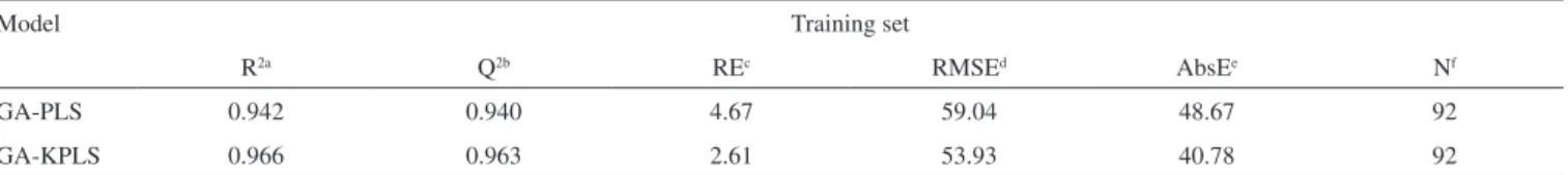
Table 3. The statistical parameters of different constructed QSRR models
Model Training set
R2a Q2b REc RMSEd AbsEe Nf
GA-PLS 0.942 0.940 4.67 59.04 48.67 92
GA-KPLS 0.966 0.963 2.61 53.93 40.78 92
a: square correlation coeficient; b: square correlation coeficient leave-group-out cross validation; c: relative error; d: root mean square error; e: absolute error; f: number of compounds in training set
Table 4. The statistical parameters of different constructed QSRR models
Model Test set
R2a REb RMSEc AbsEd Ne
GA-PLS 0.914 6.13 93.20 71.84 25 GA-KPLS 0.938 3.52 81.60 58.4 25 a: square correlation coeficient; b: relative error; c: root mean square error; d: absolute error; e: number of compounds in test set
RI by GA-KPLS versus experimental RI values for training and test set are shown Figure 1. Obviously, there is a close agreement between the experimental and predicted RI and the data represent a very low scattering around a straight line with respective slope and intercept close to one and zero. This clearly shows the strength of GA-KPLS as a nonlinear feature selection method. This result indicates that the RI of essential oils possesses some nonlinear characteristics.
Description of models descriptors
In the chromatographic retention of compounds in the polar sta-tionary phases is related to the induced forces that are very important in retention of the compounds. The induced forces are related to the dipolar moment, which should stimulate dipole-induced dipole in-teractions. Also, it is related to the dispersion forces. The dispersion forces related to steric factors, molecular size and branching. For these reasons, constitutional descriptors and electronic descriptors are very important.
Electronic descriptors were deined in terms of atomic charges and used to describe electronic aspects both of the whole molecule and of particular regions, such atoms, bonds, and molecular fragments. This descriptor calculated by computational chemistry and therefore can be consider among quantum chemical descriptor. The eigenval-ues of LUMO and HOMO and their energy gap relect the chemical activity of the molecule. LUMO as an electron acceptor represents the ability to obtain an electron, while HOMO as an electron donor represents the ability to donate an electron. HOMO energy is a useful descriptor that presents information on the distribution of π electron and explains π-π charge transfer interactions of unsaturated com-pounds. The lowest unoccupied molecular orbital (LUMO) energy can be interpreted as a measure of charge transfer interactions and/ or of hydrogen bonding effects.31,32
Constitutional descriptors are most simple and commonly used descriptors, relecting the molecular composition of a compound without any information about its molecular geometry. The most common Constitutional descriptors are number of atoms, number of bound, absolute and relative numbers of speciic atom type, ab-solute and relative numbers of single, double, triple, and aromatic bound, number of ring, number of ring divided by the number of atoms or bonds, number of benzene ring, number of benzene ring divided by the number of atom, molecular weight and average molecular weight.
Burden eigenvalues descriptors deined as eigenvalues of a modiied connectivity matrix, which could be called burden matrix
B., the B matrix representing an H-depleted molecular graph. BCUT descriptor (Burden-CAS-University of Texas eigenvalues) are based on a signiicant extension of Burden approach, considering three classes of matrices whose diagonal elements correspond to 1) atomic charge-related values, 2) atomic polarizability-related values, and 3) atomic H-bond abilities.33
Topological descriptors are based on a graph representation of the molecule. They are numerical quantiiers of molecular topol-ogy obtained by the application of algebraic operators to matrices representing molecular graphs and whose values are independent of vertex numbering or labeling. They can be sensitive to one or more structural features of the molecule such as size, shape, symmetry, branching and cyclicity and can also encode chemical information concerning atom type and bond multiplicity. Balaban index is a variant of connectivity index, represents extended connectivity and is a good descriptor for the shape of the molecules and modifying biological process. Nevertheless, some of chemists have used this index successfully in developing QSPR/QSRR models.
Charge descriptors were deined in terms of atomic charges and used to describe electronic aspects both of the whole molecule and of particular regions, such atoms, bonds, and molecular fragments. Charge descriptor calculated by computational chemistry and there-fore can be consider among quantum chemical descriptor. Electrical charges in the molecule are the driving force of electrostatic inter-actions, and it is well known that local electron densities or charge play a fundamental role in many chemical reactions, physic-chemical properties and receptors-ligand binding afinity.34
CONCLUSION
In this study, an accurate QSRR model for estimating the retention indices (RI) of essential oils from ive Pimpinella species gathered from central Turkey which obtained by GC and GC-MS was devel-oped by employing the linear model (GA-PLS) and nonlinear model (GA-KPLS). The most important molecular descriptors selected represent the electronic, charge and constitutional descriptors that are known to be important in the retention mechanism of essential oils. Two models have good predictive capacity and excellent statistical parameters. The results obtained by GA-KPLS were compared with the results obtained by GA-PLS model. The results demonstrated that GA-KPLS was more powerful in the retention indices of the essential oils than GA-PLS. This model could accurately predict the partitioning of these components that did not exist in the modeling procedure. It was easy to notice that there was a good prospect for the GA-KPLS application in the QSRR modeling.
REFERENCES
1. Burt, S.; Food Microbiol. 2004,94, 223.
2. Kim, N. S.; Lee. D. D.; J. Chromatogr., A2002, 982, 31.
3. Eminagaoglu, O.; Tepe, B.; Yumrutas, O.; Akpulat, H. A.; Daferera, D.; Polissiou, M.; Sokmen, A.; Food Chem. 2007, 100, 339.
5. Baytop, T.; Turkiyede Bitkilerle Tedavi, Nobel Tip Kitapevi, Istanbul, 1999.
6. Joulain, D.; Konig W. A.; The Atlas of Spectra Data of Sesquiterpene Hydrocarbons, E. B. Verlag: Hamburg, 1998.
7. Jennings, W.; Shibamoto, T.; Quantitative Analysis of Flavor and Fragrance Volatile by Glass Capillary Column Gas Chromatography, Academic Press: New York, 1980.
8. Ong, V. S.; Hites, R. S.; Anal. Chem. 1991, 63, 2829.
9. Peng, C. T.; Ding, S. F.; Hua, R. L.; Yang, W. C.; J. Chromatogr. 1988, 436, 137.
10. Kaliszan, R.; Structure and Retention in Chromatography, Harwood: Amsterdam, 1997.
11. Qin, L. T.; Liu, Sh. Sh.; Liu, H. L.; Tong, J.; J. Chromatogr., A 2009, 1216, 5302.
12. Noorizadeh, H.; Farmany, A.; Noorizadeh, M.; Quim. Nova2011, in press.
13. Noorizadeh, H.; Farmany, A.; Chromatographia2010, 72, 563. 14. Sauer-Leal, E.; Okada, F. M.; Peralta-Zamora, P.; Quim. Nova. 2008, 31,
1621.
15. Kaliszan, R.; J. Chromatogr., A1993, 656, 417.
16. Lindgren, F.; Geladi, P.; Wold, S.; J. Chemometrics1993,7, 45. 17. Braak, J. M.; Birks, H. J. B.; J. Chemometrics1994, 8, 169.
18. Krämer, N.; Boulesteix, A. L.; Tutz, G.; Chemom. Intell. Lab. Syst. 2008, 94, 60.
19. Tabanca, N.; Demirci, B.; Ozek, T.; Kirimer, N.; Can Baser, K. H.; Be-dir, E.; Khand, I. A.; Wedge, D. E.; J. Chromatogr., A 2006, 1117, 194. 20. Todeschini, R.; Consonni, V.; Mauri, A.; Pavan, M.; DRAGON-Software
for the calculation of molecular descriptors, version 3.0 for Windows, 2003.
21. Costa Filho, C. A.; Poppi, R. J.; Quim. Nova1999, 22, 405. 22. Lemes, M. R.; Pino Júnior, A. D.; Quim. Nova2002, 25, 539. 23. Depczynski, U.; Frost, V. J.; Molt, K.; Anal. Chim. Acta2000,420, 217. 24. Samistraro, G.; Muniz, G. I. B.; Peralta-Zamora, P.; Cordeiro, G. A.;
Quim. Nova2009, 32, 1422.
25. Nicolaï, B. M.; Theron, K. I.; Lammertyn, J.; Chemom. Intell. Lab. Syst.
2007, 85, 243.
26. Rosipal, R.; Trejo, L. J.; J. Mach. Learning Res. 2001, 2, 97. 27. Noorizadeh, H.; Farmany, A.;J. Chin. Chem. Soc. 2010,57, 1. 28. Afantitis, A.; Melagraki, G.; Sarimveis, H.; Koutentis, P. A.; Markopoulos,
J.; Igglessi-Markopoulou, O.; Bioorg. Med. Chem. 2006,14, 6686. 29. Golbraikh, A.; Tropsha, A.; J. Mol. Graphics Modell. 2002, 20, 269. 30. Kim, K.; Lee, J. M.; Lee, I. B.; Chemom. Intell. Lab. Syst. 2005,79, 22. 31. Salvi, M.; Dazzi, D.; Pelistri, I.; Neri, F.; Wall, J. R.; Ophthalmology
2002, 109, 1703.
32. Kim, K.; Lee, J. M.; Lee, I. B.; Chemom. Intell. Lab. Syst. 2005, 79, 22. 33. Booth, T. D.; Azzaoui, K.; Wainer, I. W.; Anal. Chem. 1997, 69, 3879. 34. Todeschini, R.; Consonni, V.; Handbook of molecular descriptors,