Quantitative structure-retention relationship studies for organic pollutants in textile wastewaters and landfill leachate in LC-APCI-MS

(1)

Article

Quantitative structure-retention relationship studies for organic

pollutants in textile wastewaters and landfill leachate in LC-APCI-MS

Kamyar Arman1, Ehsan Aghayani2

1

Department of Environmental Engineering, School of Agricultural Engineering, Payame Noor University, Tehran, Iran 2

Dept. of Environmental Health Engineering, Faculty of Health, Shahid Beheshti University of Medical Sciences, Tehran, Iran E-mail: [email protected]

Received 21 December 2012; Accepted 25 January 2013; Published online 1 June 2013

Abstract

A quantitative structure–retention relation (QSRR) study was conducted on the retention times of organic

pollutants in textile wastewaters and landfill leachate which obtained by liquid chromatography-reversed phase-atmospheric pressure chemical ionisation-mass spectrometry (LC-APCI-MS). The genetic algorithm was used as descriptor selection and model development method. Modeling of the relationship between

selected molecular descriptors and retention time was achieved by linear (partial least square; PLS) and nonlinear (Levenberg-Marquardt artificial neural network; L-M ANN) methods. Linear and nonlinear methods

resulted in accurate prediction whereas more accurate results were obtained by L-M ANN model. This is the first research on the QSRR of the organic pollutants in textile wastewaters and landfill leachate against the retention time.

Keywords organic pollutants; textile wastewaters; landfill leachate; LC-APCI-MS; QSRR;

Levenberg-Marquardt artificial neural network.

1 Introduction

Water pollution may be defined as the addition of any substance (pollutant) to water resource which may change the physical and chemical characteristics in any way which may interfere with its use for legitimate purposes. A great number of synthetic organic chemicals have been released to the environment due to

industrial activities. Textile wastewaters contain a wide range of non-polar and polar compounds, but polar ones are predominant. They comprise substances which are used as auxiliary products in textile production and

treatment and are washed out of the textiles having run off with the wastewater. These polar organic pollutants in textile wastewater may give rise to problems due to the fact that they are non-biodegradable and their elimination is incomplete. Moreover, some of the contaminants have a toxic effect on the bacteria applied for

wastewater purification (Covarrubias et al., 2008). As a consequence strict characterization of contaminated effluents needs to be done. In this respect the European Union (EU) has promulgated a Directive on Integrated

Environmental Skeptics and Critics ISSN 22244263

URL: http://www.iaees.org/publications/journals/environsc/onlineversion.asp RSS: http://www.iaees.org/publications/journals/environsc/rss.xml

Email: [email protected] EditorinChief: WenJun Zhang

(2)

Pollution Prevention Control (IPPC) expanding the range of pollutants that should be monitored in industrial effluents discharges (García-Pérez et al., 2010). This Directive covers many industrial sectors and it is indicated in the Directive that all the substances discharged should be monitored and the former European Union black list expanded by adding new compounds. It is of interest to the EU to develop monitoring strategies for the characterization of a variety of pollutants. From this perspective, research strategies applied

to the characterization of new pollutants in contaminated industrial effluents will be encouraged and will be expanded during the next coming years.

Another area of interest is the landfill leachates. In the EU and related European countries a total number of 250 000 abandoned and closed landfills can be estimated. From a number of investigations all over Europe, it can be estimated 50 000 landfills as hazard to the environment which already due or will pollute the

groundwater and surface water in the near future. For this reason, the recently adopted Landfill directive by the EU on 26th April 1999 requires a general improvement in the standards of landfill construction and operation

with the objective of preventing any negative effect on the environment caused by landfilling. One of the key issues in this new Directive is that monitoring of landfill leachates and surface waters affected by the landfill should be carried out (Wang et al., 2006).

Common methods for identifying organic pollutants in contaminated industrial effluents generally involve the use of either dichloromethane liquid–liquid extraction (LLE) or solid phase extraction (SPE), followed by

gas chromatography-mass spectrometry (GC-MS) techniques with electron impact (EI) ionisation (Petitgirard et al., 2009; Mothes et al., 2010; Burkhard et al., 1991; Biache et al., 2011), although few works have also

been reported using chemical ionisation (Nash et al., 2005; Covaci et al., 2005). By this approach a variety of non-polar compounds are generally determined in waste waters and effluents like phthalates, phosphates, benzenes, PAHs. However, many polar, ionic, heavy and thermally unstable compounds cannot be analysed by

GC techniques. A different approach should be used for these pollutants which usually comprise more than 95% of the organic content (Mothes et al., 2010; Biache et al., 2011).

The use of LC has been rarely reported in the characterization of polar analytes detected in industrial effluents. In this respect, few papers were published determining a variety of non-ionic and anionic surfactants in waste waters (Gutiérrez et al., 2007; Gomez et al., 2001). The US EPA has published two methods for the

analysis of solid waste (SW-846), involving either particle beam (method 8325) (Huang et al., 2005) or thermospray (method 8321) (US EPA, 1995). These methods involve the determination of different kinds of

pollutants including disperse azo dyes, phosphates, pesticides and benzidines in waste waters. Both methods were recently applied to the characterisation of many organic acids found in Superfund sites (Mothes et al., 2010)

LC-TSP-MS was used to confirm that approximately half of the unidentified total organic halocarbon (TOX) content in leachates from a hazardous waste site is 4-chlorobenzene sulfonic acid. However, the main obstacle

to routine analytical applications of LC-MS has been the unavailability of rugged and reliable LC-MS interfaces. The development of atmospheric pressure ionization (API) LC-MS interfaces provides structural information similar to that obtained by chemical ionization techniques, overcoming the limitations of other

LC-MS interfacing devices such as poor structural information or sensitivity related to TSP and PB, respectively. Recently, reported the use of LC-APCI-MS combined with toxicity-based fractionation using

Vibrio fsicheri for the characterisation of organic pollutants in waste water treatment works (Castillo and Barceló, 1999). In addition to the toxicity-based fractionation, a sequential solid phase extraction (SSPE) protocol was also applied to the raw samples to identify the major organic pollutants present. The final

(3)

In addition to that chromatographic retention prediction methodologies can be valuable starting points for GC method development. A promising approach is the use of quantitative structure–retention relationship

(QSRR) (Put and Heyden, 2007; Kaliszan, 1997). QSRR are statistically derived relationships between chromatographic parameters and descriptors related to the molecular structure of the analytes. In QSRR these descriptors are used to model the molecular interaction of the analytes with a given stationary phase and eluent

(Baczek and Kaliszan, 2002). In chromatography, QSRR have been applied to: (i) gain a better understanding of the molecular mechanism of the chromatographic separation process; (ii) identify the most informative structure related properties of analytes; (iii) characterize stationary phases, and (iv) predict retention for new analytes (Put and Heyden, 2007).

There is a trend to develop QSRR from a variety of methods. In particular, genetic algorithm (GA) is

frequently used as search algorithms for variable selection in chemometrics and QSRR. The GA provides a “population” of models, from which it could be difficult to identify the most significant or relevant models

(which may be preferred in certain uses, e.g. regulatory toxicology prediction) (Hewitt et al., 2007).

Partial least square (PLS) is the most commonly used multivariate calibration method. Moreover, non-linear statistical treatment of QSRR data is expected to provide models with better predictive quality as

compared with related PLS models.

Moreover, non-linear statistical treatment of QSRR data is expected to provide models with better predictive

quality as compared with linear models. In this perspective, artificial neural network (ANN) modelling has become quite common in the QSRR field (Noorizadeh and Farmany, 2010). Extensive use of ANN, which does not

require the “a priori” knowledge of the mathematical form of the relationship between the variables, largely rests on its flexibility functions of any complexity can be apply. In the present work, a QSRR study has been carried out on the liquid chromatography-reversed phase-atmospheric pressure chemical ionisation- mass

spectrometry (LC-APCI-MS) system retention times (tR) for organic pollutants in textile wastewaters and landfill leachate by using structural molecular descriptors. The present study is a first research on QSRR of the organic pollutants in textile wastewaters and landfill leachate against the tR, using GA-PLS and L-M ANN.

2 Materials and Methods 2.1 Data set

Retention time (tR) of 35 organic pollutants in textile wastewaters and landfill leachate which obtained by LC-APCI-MS were taken from the literature (Castillo and Barceló, 2001) is shown in Table 1. The retention time

of these compounds were increased in the range of 5.07 and 33.47 for both Phenol and Dotriacontane, respectively.

2.2. LC-APCI-MS conditions

Samples were collected in Pyrex borosilicate glass containers. Each bottle was rinsed with tap water and with high-purity water prior to sample addition. For LC-APCI-MS experiments a VG Platform from Micromass

(Manchester, UK) equipped with a standard atmospheric pressure ionisation (API) source, which can be configurated for APCI or ESI, was used. Mobile phase of water and acetonitrile both acidified with 0.5% of

acetic acid was used to accomplish separation on an Hypersil Green ENV column (150mm



4.6mm i.d., 5



m particle size) equipped with a guard column both from Shandon HPLC (Cheshire, UK).

Source and probe temperatures were set at 150 and 400oC, respectively, corona discharge voltage was

(4)

checked. In order to distinguish between the different functionalities, the presence of peaks at m/z 151 and 195 were checked for aliphatic alcohol polyethoxylate, AEOn,x; at m/z 271 and 291 for nonylphenol polyethoxylate

NPEOx and at m/z 101 and 145 for PEGx . In addition to this comparison, non-ionic polyethoxylated

surfactants were identified by checking correspondence

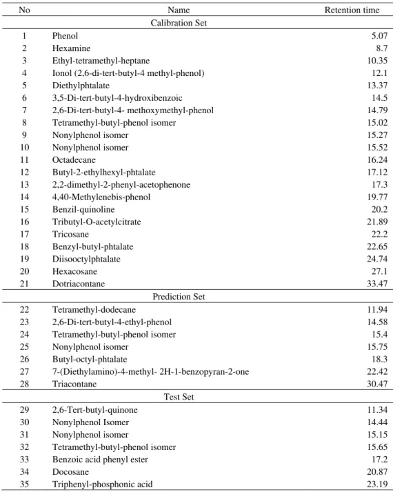
Table 1 The data set, structure and the corresponding observed retention time values.

No Name Retention time

Calibration Set

1 Phenol 5.07

2 Hexamine 8.7

3 Ethyl-tetramethyl-heptane 10.35

4 Ionol (2,6-di-tert-butyl-4 methyl-phenol) 12.1

5 Diethylphtalate 13.37

6 3,5-Di-tert-butyl-4-hydroxibenzoic 14.5

7 2,6-Di-tert-butyl-4- methoxymethyl-phenol 14.79

8 Tetramethyl-butyl-phenol isomer 15.02

9 Nonylphenol isomer 15.27

11 Octadecane 16.24

12 Butyl-2-ethylhexyl-phtalate 17.12

13 2,2-dimethyl-2-phenyl-acetophenone 17.3

14 4,40-Methylenebis-phenol 19.77

15 Benzil-quinoline 20.2

16 Tributyl-O-acetylcitrate 21.89

17 Tricosane 22.2

18 Benzyl-butyl-phtalate 22.65

19 Diisooctylphtalate 24.74

20 Hexacosane 27.1

21 Dotriacontane 33.47

Prediction Set

22 Tetramethyl-dodecane 11.94

23 2,6-Di-tert-butyl-4-ethyl-phenol 14.58

26 Butyl-octyl-phtalate 18.3

27 7-(Diethylamino)-4-methyl- 2H-1-benzopyran-2-one 22.42

28 Triacontane 30.47

Test Set

29 2,6-Tert-butyl-quinone 11.34

30 Nonylphenol Isomer 14.44

33 Benzoic acid phenyl ester 17.2

34 Docosane 20.87

35 Triphenyl-phosphonic acid 23.19

2.3 GC-MS characterisation of toxicity fractionated extracts

The inherent low volatility of several pollutants such as the non-ionic surfactants, hampered the application of HRGC for their analysis. This fact was overcome by the use of high temperature capillary columns and a cold

(5)

textile effluents) are shown in Table 1. Fast characterization of a great number of different classes of pollutants, including highly functionalised compounds, such as tetraethoxyphenol was possible. This revealed the

presence of various groups of chemical components in industrial effluents such as phenolic compounds, phthalates, aliphatic carboxylic acids, aromatic carboxylic acids, amines, alkanes and linear aliphatic alcohols among them.

Aliphatic carboxylic acids were detected from C8 to C18 with two different origins: the short chain

carboxylic acids of metabolic origin and the long chain fatty acids of the hides, fatting agents and microbial

biomass. Aromatic carboxylic acids were also present in the studied wastewaters as constituents of natural tanning agents. Amines and linear aliphatic alcohols are regularly determined in industrial effluents due to their use in the production of dyes and textiles and as solvents and antifoaming agents, respectively.

2.4 Molecular modeling and theoretical molecular descriptors

The derivation of theoretical molecular descriptors proceeds from the chemical structure of the compounds. In

order to calculate the theoretical descriptors, molecular structures were constructed with the aid of HyperChem version 7.0. The final geometries were obtained with the semi-empirical AM1 method in HyperChem program. The molecular structures were optimized using Fletcher- Reeves algorithm until the root mean square gradient

was 0.01 kcal mol-1. Some quantum descriptor such as orbital energy of LUMO was calculated by using the HyperChem software. The resulted geometry was transferred into Dragon program, to calculate 1497

descriptors, which was developed by Todeschini et al (Todeschini et al., 2003). To reduce the original pool of descriptors to an appropriate size, the objective descriptor reduction was performed using various criteria. Reducing the pool of descriptors eliminates those descriptors which contribute either no information or whose

information content is redundant with other descriptors present in the pool.

2.5 Genetic algorithm for descriptor selection

To select the most relevant descriptors with GA, the evolution of the population was simulated (Ferrand et al., 2011). Each individual of the population, defined by a chromosome of binary values, represented a subset of descriptors. The number of the genes at each chromosome was equal to the number of the descriptors. The

population of the first generation was selected randomly. A gene was given the value of one, if its corresponding descriptor was included in the subset; otherwise, it was given the value of zero. The number of

the genes with the value of one was kept relatively low to have a small subset of descriptors (Aires-de-Sousa et al., 2002) that is the probability of generating zero for a gene was set greater. The operators used here were crossover and mutation. The application probability of these operators was varied linearly with a generation

renewal. For a typical run, the evolution of the generation was stopped, when 90% of the generations had taken the same fitness. The molecules of the training and the test sets, on which the GA technique was performed,

are shown in Table 1. In this paper, size of the population is 30 chromosomes, the probability of initial variable selection is 5:V (V is the number of independent variables), crossover is multi Point, the probability of crossover is 0.5, mutation is multi Point, the probability of mutation is 0.01 and the number of evolution

generations is 1000. For each set of data, 3000 runs were performed.

2.6 Nonlinear model: Artificial neural network

An artificial neural network (ANN) with a layered structure is a mathematical system that stimulates biological neural network, consisting of computing units named neurons and connections between neurons named synapses (Kara et al., 2006; Zhang and Barrion, 2006; Kara and Okandan, 2007; Zhang, 2007; Zhang et al.,

2007; Zhang et al., 2008a, b; Zhang and Zhang, 2008; Zhang and Wei, 2009; Noorizadeh et al., 2011; Watts, 2011; Watts and Worner, 2011; Zhang, 2010, 2011). All feed-forward ANN used in this paper are three-layer

(6)

Input layer

Hidden layer

Output layer

ANN training and the linear functions were used as the transformation functions in hidden and output layers.

3 Results and Discussion 3.1 Linear model

To reduce the original pool of descriptors to an appropriate size, the objective descriptor reduction was

performed using various criteria. Reducing the pool of descriptors eliminates those descriptors which contribute either no information or whose information content is redundant with other descriptors present in

the pool. The remained descriptors were employed to generate the models with the GA-PLS program. The best model is selected on the basis of the highest square correlation coefficient leave-group-out cross validation (R2), the least root mean squares error (RMSE) and relative error (RE) of prediction. These parameters are

probably the most popular measure of how well a model fits the data. The best GA-PLS model contains eleven selected descriptors in three latent variables space. These descriptors were obtained constitutional descriptors

(sum of atomic polarizabilities (scaled on Carbon atom) (Sp) and (number of bonds (nBT)), topological descriptors (quasi-Wiener index (Kirchhoff number) (QW), Wiener-type index from mass weighted distance matrix (Whetm) and mean distance degree deviation (MDDD)), 2D autocorrelations (Moran autocorrelation -

lag 4 / weighted by atomic masses (MATS4m)), geometrical descriptors (3D-Wiener index (W3D), absolute eigenvalue sum on geometry matrix (SEig)), functional group counts (number of total tertiary C(sp3) (nCt)),

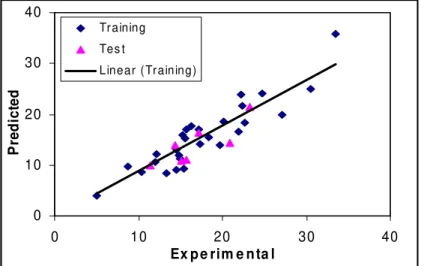
charge descriptors (total positive charge (Qpos)) and quantum chemical descriptors (lowest unoccupied molecular orbital (LUMO)). The R2 and mean RE for training and test sets were (0.827, 0.709) and (15.44, 22.91), respectively. The predicted values of tR are plotted against the experimental values for training and test

sets in Fig 2. For this in general, the number of components (latent variables) is less than the number of independent variables in PLS analysis. The PLS model uses higher number of descriptors that allow the model

to extract better structural information from descriptors to result in a lower prediction error.

Fig. 1 Used three layer ANN.

3.2 Nonlinear model

With the aim of improving the predictive performance of nonlinear QSRR model, L-M ANN modeling was performed. The networks were generated using the twelve descriptors appearing in the GA-PLS models as

(7)

and prediction (training) and test sets. All molecules were randomly placed in these sets. A three-layer network with a sigmoid transfer function was designed for each ANN. Before training the networks the input and

output values were normalized between -1 and 1. The network was then trained using the training set by the back propagation strategy for optimization of the weights and bias values. The procedure for optimization of the required parameters is given elsewhere (Jalali-Heravi et al., 2004). The proper number of nodes in the

hidden layer was determined by training the network with different number of nodes in the hidden layer. The root-mean-square error (RMSE) value measures how good the outputs are in comparison with the target values.

It should be noted that for evaluating the overfitting, the training of the network for the prediction of tR must stop when the RMSE of the prediction set begins to increase while RMSE of calibration set continues to decrease. Therefore, training of the network was stopped when overtraining began. All of the above mentioned

steps were carried out using basic back propagation, conjugate gradient and Levenberge-Marquardt weight update functions. It was realized that the RMSE for the training and test sets are minimum when four neurons

were selected in the hidden layer and the learning rate and the momentum values were 0.8 and 0.4, respectively. Finally, the number of iterations was optimized with the optimum values for the variables. It was realized that after 18 iterations, the RMSE for prediction set were minimum.

0 10 20 30 40

Ex p e rim e n ta l

Pr

e

d

ic

te

d

Training Tes t

Linear (Training)

Fig. 2 Plots of predicted retention time against the experimental values by GA-PLS model.

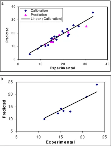
The R2 and RE for calibration, prediction and test sets were (0.931, 0.924, 0.906) and (8.50, 10.27, 13.19),

respectively. Inspection of the results reveals a higher R2 and lowers other values parameter for the test set compared with their counterparts for other models. Plots of predicted tR versus experimental tR values by L-M

ANN for calibration, prediction and test sets are shown in Fig. 3a, 3b, respectively. The relative error and R2 of test set for the GA-PLS model are 22.91 and 0.709 respectively which would be compared with the values of 13.19 and 0.906, respectively, for the L-M ANN model. Comparison between these values and other statistical

parameters reveals the superiority of the L-M ANN model over other model. The key strength of neural networks, unlike regression analysis, is their ability to flexible mapping of the selected features by

manipulating their functional dependence implicitly. The statistical parameters reveal the high predictive ability of L-M ANN model. The whole of these data clearly displays a significant improvement of the QSRR model consequent to nonlinear statistical treatment. Obviously, there is a close agreement between the

(8)

respective slope and intercept close to one and zero. As can be seen in this section, the L-M ANN is more reproducible than GA-PLS for modeling the LC-APCI-MS retention time of organic pollutants in textile

wastewaters and landfill leachate.

0 10 20 30 40

Exp e r im e n t al

Pre

d

ic

te

d

Calibration Predic tion

Linear (Calibr ation)

a

5 10 15 20 25

Ex p e rim e n ta l

Pr

e

d

ic

te

d

b

Fig. 3 Plot of predicted tR obtained by L-M ANN against the experimental values (a) calibration and prediction sets of molecules and (b) for test set.

3.3 Model validation and statistical parameters

The applied internal (leave-group-out cross validation (LGO-CV)) and external (test set) validation methods were used for the predictive power of models. In the leave-group-out procedure one compound was removed from the data set, the model was trained with the remaining compounds and used to predict the discarded

compound. The process was repeated for each compound in the data set. The predictive power of the models developed on the selected training set is estimated on the predicted values of test set chemicals. The data set

should be divided into three new sub-data sets, one for calibration and prediction (training), and the other one for testing. The calibration set was used for model generation. The prediction set was applied deal with overfitting of the network, whereas test set which its molecules have no role in model building was used for

the evaluation of the predictive ability of the models for external set.

In the other hand by means of training set, the best model is found and then, the prediction power of it is

(9)

components are in calibration set, 7 components are in prediction set and 21 components are in test set).

The result clearly displays a significant improvement of the QSRR model consequent to non-linear

statistical treatment and a substantial independence of model prediction from the structure of the test molecule. In the above analysis, the descriptive power of a given model has been measured by its ability to predict partition of unknown organic pollutants in textile wastewaters and landfill leachate.

For the constructed models, some general statistical parameters were selected to evaluate the predictive ability of the models for tR values. In this case, the predicted tR of each sample in prediction step was

compared with the experimental acidity constant. Root mean square error (RMSE) is a measurement of the average difference between predicted and experimental values, at the prediction step. RMSE can be interpreted as the average prediction error, expressed in the same units as the original response values. Its small value

indicates that the model predicts better than chance and can be considered statistically significant. The RMSE was obtained by the following formula:



 





n i i i

y

n

RMSE

1 2 1 2

]

)

(

1 [

(1)

The other statistical parameter was relative error (RE) that shows the predictive ability of each component, and is calculated as:





















  n i i i i

y

n

RE

1 0

0

₎

₁₀₀

1 (

)

(

(2)

The predictive ability was evaluated by the square of the correlation coefficient (R2) which is based on the

prediction error sum of squares and was calculated by following equation:



  





_n i i i n i

y

R

1 _ _ 1 2

)

(

)

(

(3)

where yi is the experimental tR in the sample i, y_i



represented the predicted tR in the sample i,

_

y

is the mean

of experimental tR in the prediction set and n is the total number of samples used in the test set.

The main aim of the present work was to assess the performances of GA-PLS and L-M ANN for modeling

the retention time of compounds. The procedures of modeling including descriptor generation, splitting of the data, variable selection and validation were the same as those performed for modeling of the retention time of organic pollutants in textile wastewaters and landfill leachate.

4 Conclusion

(10)

methods seemed to be useful, although a comparison between these methods revealed the slight superiority of the L-M ANN over the model. High correlation coefficients and low prediction errors confirmed the good

predictability of two models. Application of the developed model to a testing set of 30 compounds demonstrates that the new model is reliable with good predictive accuracy and simple formulation. The QSRR procedure allowed us to achieve a precise and relatively fast method for determination of tR of different series

of organic pollutants to predict with sufficient accuracy the tR of new compound derivatives. To the best of our knowledge this is the first study for the prediction of retention time of organic pollutants in textile wastewaters

and landfill leachate using GA-PLS and L-M ANN.

References

Aires-de-Sousa J, Hemmer MC, Casteiger J. 2002. Prediction of H-1 NMR chemical shifts using neural

networks. Analytical Chemistry 74: 80-90

Aschi M, D’Archivio AA, Maggi MA, et al. 2007. Quantitative structure-retention relationships of pesticides in reversed-phase high-performance liquid chromatography. Analytica Chimica Acta, 582(2): 235-242

Baczek T, Kaliszan R. 2002. Combination of linear solvent strength model and quantitative structure-retention relationships as a comprehensive procedure of approximate prediction of retention in gradient liquid

chromatography. Journal of Chromatography A, 962: 41-45

Biache C, Ghislain T, Faure P, et al. 2011. Low temperature oxidation of a coking plant soil organic matter and its major constituents: An experimental approach to simulate a long term evolution. Journal of

Hazardous Materials, 188: 221-230

Boysen RI, Milton TW. 2010. High performance liquid chromatographic separation methods. In:

Comprehensive Natural Products II. 5-49

Burkhard LP, Durhan EJ, Lukasewycz MT. 1991. Identification of nonpolar toxicants in effluents using toxicity-based fractionation with gas chromatography/mass spectrometry. Analytical Chemistry, 63:

277-283

Castillo M, Barceló D. 1999. Identification of polar toxicants in industrial wastewaters using toxicity-based

fractionation with liquid chromatography/mass spectrometry. Analytical Chemistry, 71: 3769-3776

Castillo M, Barceló D. 2001. Characterisation of organic pollutants in textile wastewaters and landfill leachate by using toxicity-based fractionation methods followed by liquid and gas chromatography coupled to mass

spectrometric detection. Analytica Chimica Acta, 426: 253-264

Castillo M, Barceló D, Pereira AS, et al. 1999. Characterization of organic pollutants in industrial effluents by

high-temperature gas chromatography–mass spectrometry. Trends in Analytical Chemistry, 18: 26-36 Covaci A, Gheorghe A, Voorspoels S, et al. 2005. Polybrominated diphenyl ethers, polychlorinated biphenyls

and organochlorine pesticides in sediment cores from the Western Scheldt river (Belgium): analytical

aspects and depth profiles. Environment International, 31: 367-375

Covarrubias C, García R, Arriagada R, et al. 2008. Removal of trivalent chromium contaminant from aqueous

media using FAU-type zeolite membranes. Journal of Membrane Science, 312: 163-173

Ferrand M, Huquet B, Barbey S, et al. 2011. Determination of fatty acid profile in cow's milk using mid-infrared spectrometry: Interest of applying a variable selection by genetic algorithms before a PLS

regression. Chemometrics and Intelligent Laboratory Systems, 106: 183-189

Fragkaki AG, Tsantili-Kakoulidou A, Angelis YS, et al. 2009. Gas chromatographic quantitative structure–

(11)

García-Pérez J, López-Cima MF, Boldo E, et al. 2010. Leukemia-related mortality in towns lying in the vicinity of metal production and processing installations. Environment International, 36: 746-753

Gomez V, Ferreres L, Pocurull E, et al. 2011. Determination of non-ionic and anionic surfactants in environmental water matrices. Talanta, 84: 859-866

Gutiérrez G, Cambiella A, Benito JM, et al. 2007. The effect of additives on the treatment of oil-in-water

emulsions by vacuum evaporation. Journal of Hazardous Materials, 144: 649-654

Hewitt M, Cronin MTD, Madden JC, et al. 2007. Consensus QSAR models: Do the benefits outweigh the

complexity? Journal of Chemical Information and Modeling, 47: 1460-1468

Huang KC, Zhao ZQ, Hoag GE, et al. 2005. Degradation of volatile organic compounds with thermally activated persulfate oxidation. Chemosphere, 61: 551-560

Jalali-Heravi M, Noroozian E, Mousavi E. 2004. Prediction of relative response factors of electron-capture detection for some polychlorinated biphenyls using chemometrics. Journal of Chromatography A, 1023(2):

247-254

Kara S, Güven AS, Okandan M, et al. 2006. Utilization of artificial neural networks and autoregressive modeling in diagnosing mitral valve stenosis. Computers in Biology and Medicine, 36: 473-483

Kara S, Okandan M. 2007. Atrial fibrillation classification with artificial neural networks. Pattern Recognition, 40: 2967-2973

Karen CW, Alberico BF. 2008. A chemometric study of the 5HT 1A receptor affinities presented by arylpiperazine compounds. European Journal of Medicinal Chemistry, 43(2): 364-372

Kaliszan R. 1997. Structure, Retention in Chromatography. A Chemometric Approach. Harwood Academic Publishers, Amsterdam, Netherlands

Mothes F, Reiche N, Fiedler P, et al. 2010. Capability of headspace based sample preparation methods for the

determination of methyl tert-butyl ether and benzene in reed (phragmites australis) from constructed wetlands. Chemosphere, 80: 396-403

Nash D, Leeming R, Clemow L, et al. 2005. Quantitative determination of sterols and other alcohols in overland flow from grazing land and possible source materials. Water Research, 39: 2964-2978

Noorizadeh H, Farmany A. 2010. QSRR models to predict retention indices of cyclic compounds of essential

oils. Chromatographia, 72: 563-569

Noorizadeh H, Farmany A, Noorizadeh M. 2011. Quantitative structure retention relationship analysis

retention index of essential oils. Quimica Nova, 34(2): 242-249

Petitgirard A, Djehiche M, Persello J, et al. 2009. PAH contaminated soil remediation by reusing an aqueous solution of cyclodextrins. Chemosphere, 75: 714-718

Put R, Heyden YV. 2007. Review on modelling aspects in reversed-phase liquid chromatographic quantitative structure-retention relationships. Analytica Chimica Acta, 602: 164-172

Ruggieri F, D’Archivio AA, Carlucci G, et al. 2005. Application of artificial neural networks for prediction of retention factors of triazine herbicides in reversed-phase liquid chromatography. Journal of

Chromatography A, 1076: 163-169

Todeschini R, Consonni V, Mauri A, et al. 2003. DRAGON-Software for the calculation of molecular descriptors; Version 3.0 for Windows.

US EPA. 1995. Method 8321A, Solvent extractable nonvolatile compounds by high performance liquid chromatography/ particle beam/mass spectrometry (HPLC/PB/MS) or ultraviolet (UV) detection. 1-50, US EPA, Office of Solid Waste and Emergency response, Washington DC, USA

(12)

177-182

Watts MJ. 2011. Using data clustering as a method of estimating the risk of establishment of bacterial crop

diseases. Computational Ecology and Software, 1(1): 1-13

Watts MJ, Worner SP. 2011. Improving cluster-based methods for investigating potential for insect pest species establishment: region-specific risk factors. Computational Ecology and Software, 1(3): 138-145

Zhang WJ. 2007. Supervised neural network recognition of habitat zones of rice invertebrates. Stochastic Environmental Research and Risk Assessment, 21: 729-735

Zhang WJ. 2010. Computational Ecology: Artificial Neural Networks and Their Applications. World Scientific, Singapore

Zhang WJ. 2011. Simulation of arthropod abundance from plant composition. Computational Ecology and

Software, 1(1): 37-48

Zhang WJ, Bai CJ, Liu GD. 2007. Neural network modeling of ecosystems: a case study on cabbage growth

system. Ecological Modelling, 201: 317-325

Zhang WJ, Barrion AT. 2006. Function approximation and documentation of sampling data using artificial neural networks. Environmental Monitoring and Assessment, 122: 185-201

Zhang WJ, Liu GH, Dai HQ. 2008a. Simulation of food intake dynamics of holometabolous insect using functional link artificial neural network. Stochastic Environmental Research and Risk Assessment, 22(1):

123-133

Zhang WJ, Wei W. 2009. Spatial succession modeling of biological communities: a multi-model approach.

Environmental Monitoring and Assessment, 158: 213-230

Zhang WJ, Zhong XQ, Liu GH. 2008b. Recognizing spatial distribution patterns of grassland insects: neural network approaches. Stochastic Environmental Research and Risk Assessment, 22(2): 207-216