Braz. j. oceanogr. vol.60 número3

REMOTE WIND STRESS INFLUENCE ON MEAN SEA LEVEL IN A

SUBTROPICAL COASTAL REGION

Mabel Calim Costa1* and Marcos Eduardo Cordeiro Bernardes2

Instituto Nacional de Pesquisas Espaciais

(Rodovia Presidente Dutra, Km 39, Cachoeira Paulista, SP, Brasil)

Universidade Federal de Itajubá - Instituto de Recursos Naturais (Avenida BPS, Itajubá – MG, Brasil)

*Corresponding author: [email protected]

A

The purpose of this study was to assess the relative influence of remote wind stress on mean sea level (MSL) variations in the coastal region of Cananeia (Sao Paulo State, Southern Brazil) during the period from 1/1/1955 to 12/31/1993. An optimized low-pass Thompson filter for the study area, and spectral analysis (cross spectrum, coherence and phase lag) of the relationship between the MSL and both parallel (T//) and perpendicular (T|) wind stress components were applied. These were extracted from four grid points of the NCEP/NCAR global model. The predominance of annual oscillations as those of greatest coherence and energy, of periods of approximately 341 days (frequency of 0.00293 cpd) and 410 days (frequency of 0.00244 cpd), respectively, were observed. Offshore NCEP/NCAR grid points were those with the highest coherence and energy throughout the study in relation to the observed MSL. This may be linked to the restriction of the NCEP/NCAR model as regards the inland limit. It is also concluded that remote wind stress may play an important role in several MSL time scales, including the annual ones. Based on criteria such as coherence and energy peaks, the wind stress component of greatest effect on MSL was the parallel one.

R

O presente estudo tem por objetivo avaliar a influência relativa de tensão do vento remoto na variação do nível médio do mar (NMM) para a região costeira de Cananéia (SP) durante o período de 1/1/1955 a 31/12/1993. Foram aplicados um filtro de passa-baixa de Thompson (1983), otimizado para a região de Cananéia, além de análise espectral (espectro cruzado, coerência e defasagem) entre o NMM e as componentes paralela (T//) e perpendicular (T|) da tensão do vento. Estas foram extraídas de quatro pontos de grade do modelo global NCEP/NCAR. Observou-se a predominância das oscilações anuais como aquelas de maior coerência e energia, destacando-se os períodos de aproximadamente 341 dias (frequência de 0,00293 cpd) e 410 dias (frequência de 0,00244 cpd), respectivamente. As maiores coerências e energia em todo estudo foram encontradas nos pontos mais distantes da costa. Este fato pode estar associado às restrições do modelo NCEP/NCAR em representar os limites continentais. Conclui-se também que a tensão do vento remoto pode ter um papel importante em várias escalas temporais do NMM, incluindo a escala anual. A partir dos valores de coerência e picos energéticos, a componente paralela da tensão do vento foi a que mostrou ser mais influente no NMM da região estudada.

Descriptors: Thompson filter, Spectral analysis, NCEP/NCAR, Cananeia, Brazil. Descritores: Filtro de Thompson, Análise espectral, NCEP/NCAR, Cananéia; Brasil.

I

Given the difficulty encountered in describing phenomena occurring at the ocean-atmosphere interface, as well as in determining the correlation between meteorological and oceanographic data, the variability of mean sea level (MSL), within the context of the global warming and climate change

The investigation of MSL variability has been the focus of several studies around the world due to various factors: its effects along coastal areas, changes in coastal morphodynamic patterns, adjustment of the shoreline profile and the modification of saline intrusion into coastal aquifers (NEVES, 2005). Pugh (1996) reviewed the main concepts and methodologies for MSL and tidal analyses. In Brazil, Mesquita (2002, 2009) studied MSL variability in the light of the main tide gauges along the country´s coast. Neves (2005) and Neves and Muehe (2008) undertook the analysis of different methodologies for estimating MSL and studied its variability along the Brazilian coastline in the context of climate change. Harari and Camargo (1994, 1995) and Harari et al. (2004) studied the variation of MSL particularly at Santos and Cananeia, both on the Sao Paulo State coast. Cananeia was also the object of a NOAA (1997) study, which presented long term cycles in the region between 1955 and 2005. Camargo and Harari (1994) and Camargo et al. (1998, 1999) studied the variability of the MSLin those areas by means of numerical models.

Improvements in MSL prediction are closely related to the advance of filtering numerical methods, since MSL can be defined as the observed sea level if inertial, gravitational and ‘high’ frequency disturbances (such as diurnal, semidiurnal, terdiurnal astronomic tidal constituents, etc.) are removed. Table 1 gives an example of the filtering process used to obtain MSL on the southeastern and southern coast of Brazil by Uaissone (2004 apud Oliveira, 2007) and Oliveira (2009). Duchon (1979) described a Fourier method for filtering time series by adding a ’sigma’

factor as a means to minimize Gibbs'[1] phenomenon. The Lanczos filter as it is called is the method most commonly used in oceanography to predict MSL, mainly due to the simplicity of its implementation. Thompson (1983) proposed a filter that allows the user to choose cut-off frequencies. Despite some complexity in its implementation, Thompson´s filter seems more versatile, since it provides an optimized treatment of MSL series.

Several Brazilian authors have applied the low-pass filter proposed by Thompson (1983): i) compared data from the Rio de Janeiro State Tide Gauge Network with meteorological data extracted from the global model of NCEP/NCAR; ii) Oliveira et al. (2007) studied the effect of storm surges in Paranagua Bay (PR) and their effects on tidal records from Cananeia (SP); iii) compared Lanczos and Thompson filters' performances in the analysis of MSL variability in the coastal region of Cananeia, and iv) Oliveira et al. (2009) analyzed the response of the coastal sea level to atmospheric phenomena through the use of wind and atmospheric pressure data based on the NCEP/NCAR model and tide gauge data from Cananeia (SP). The choice of the Thompson low-pass filter in this study is mainly to be explained as due to its better performance than that shown by Lanczos' results (COSTA; BERNARDES, 2010) and to its versatility in allowing the user to determine the frequencies to be attenuated in the filtering process.

The purpose of this study is to evaluate the influence of remote wind stress on MSL variations along the coastal region of Cananeia, in southern São Paulo State, southeastern Brazil (Fig. 1).

Table 1. Statistical results of sea level (SL) and MSL (in cm) for the region of Piraquara(RJ), Ponta da Armação (RJ) and Paranaguá (PR). Sources: Uaissone (2004), Oliveira (2004) and Oliveira (2009a).

Level Average Maximum Minimum Standard

deviation

Variance Filtering

Piraquara (RJ) Original (SL)

119 215.6 17.1 32.6 1060.7

MSL 119 175.7 36.4 16.6 275.5 26%

Ponta da Armação (RJ)

Original (SL)

185.5 329 74 32.1 1024

MSL - - - - 210 21%

Paranagua (PR) Original (SL)

52.04 2705.19

MSL - - - 18.19 332.71 12%

__________

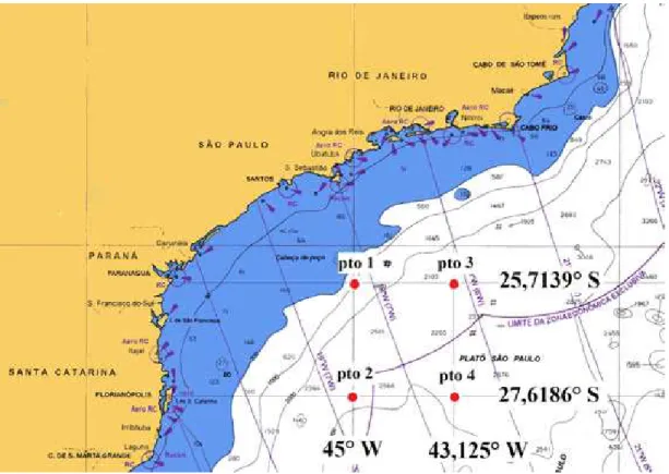
Fig. 1. Study area location (in detail) and the sampling points of the Reanalysis grid model of NCEP/NCAR. DHN – Brazilian Navy Nautical Chart Nº 1 (1995).

M

M

Sea level observations were based on tide gauge series sampled at the Oceanographic Institute of Sao Paulo University's base in Cananeia (SP), as the Institute ensures the quality of maintenance and altimetric reference over the years, with hourly measurements, from 1955 to 1993.

Meteorological data were extracted from the Reanalysis Project of NCEP/NCAR (http://www.ncep.noaa.gov), by which the zonal (Tx) and meridional (Ty) components of wind stress were estimated at 10 m above sea level with grid spacing equal to 1.875º (lat) by 1.905º (long), available at the synoptic times of 00:00, 06:00, 12:00 and 18:00 GMT. Four grid points near the study area were chosen for the space-time evaluation of tide gauge and meteorological series (Fig. 2). These data were acquired by direct access to the files on extensions such as html, netcdf and others. In this study, the second option was chosen, the data being manipulated through an Excel® macro function. The

properties of the reanalysis records are described in detail in Kalnay et al. (1996). In addition to the time series analysis against MSL data, wind model estimates were evaluated at four grid points (the closest and most relevant to the region) chosen from the NCEP/NCAR global model, and these were arranged as in Figure 2: points 1 and 2 being closer to the coast, and points 3 and 4, further offshore.

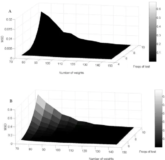
Figs 2a,b. Mean squared deviations as a function of weights number (N) and the frequency band. Without any preset frequencies to be attenuated (A). With the imposition of the 16 local main tidal components (B).

Numerical Filtering

The low-pass filter was used to obtain MSL in order to suppress the astronomical and inertial tidal components preserving the ‘low’ frequency signal (periods longer than three days) - a methodology similar to that used by Oliveira et al. (2007).

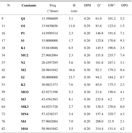
Thompson's (1983) low-pass filter allows its optimization by the user, who defines the main parameters of calculation, especially by imposing pre-selected cut-off frequencies. The harmonic components were extracted from Mesquita (1997), who analyzed the records of sea level in the coastal regions of southeastern Brazil through the application of the harmonic method developed by Franco and Rock (1971). The selected components were Q1, O1,

P1, K1, N2, M2, S2 and M3, which correspond to approximately 90% of the tidal energy on the Cananeia coast (PICARELLI et al., 2002). All the constants were determined at confidence intervals of 95% (MESQUITA, 1997), as can be seen in Table 2.

The filter equation is described by the convolution of weights over the time series in the frequency domain (i.e. a Fourier Transform), seen in details in Thompson (1983). The main parameters for optimization are: number of weights, the number of frequencies to be attenuated, lower cut-off frequency (Ω1) and upper cut-off frequency (Ω2), which defines the band to be filtered out. It should be noted that the filtering process is not perfect (EMERY; THOMSON, 2001). In other words, there is no exact, perfect answer for all the frequencies that should hold

A

intact nor a null answer for those intended to be attenuated. The ability of a filter to resolve sequential events is inversely proportional to the bandwidth, i.e. the narrower the bandwidth, the longer the time series needed to resolve individual events (EMERY; THOMSON, 2001).

Spectral Analysis

The main purpose of time series analysis methods is to define the variability of the data in terms of dominant periodic functions, or pattern recognition. In order to apply a spectral analysis, the first care to be taken is to extract, a priori, the trend and the average of the time series since the aim is to avoid distortions in the ‘low’ frequency components of the spectrum. At the same time, the time series to be analyzed must be ideally long enough to allow for many cycles of the lowest frequency of interest. This phenomenon is

known as aliasing and can be solved by filtering data in order to separate out only the fluctuations of interest, reducing the amount of adjacent frequencies that may distort the energy values of the signal (EMERY; THOMSON, 2001). These authors also state that sampling the signal also interferes in obtaining spectral estimates; for instance, an hourly series collected on a single day cannot fully describe the behavior of a daily cycle, just as monthly series over one year are not sufficient to describe an annual cycle.

Cross-spectral analysis is used to measure the degree of relationship between two stochastic processes. In this case, the covariance function between time series, described in detail in Franco (1982), Kumaresan (1993) and Emery and Thomson (2001), was applied.

Table 2. Tidal harmonic constants for Cananeia calculated from records obtained in 1978. The first column contains the name of the components; the second, the angular frequency; the third, the angular frequency in hertz; the fourth, the amplitude, in meters; the fifth, the standard deviation of amplitude; the sixth, the phase angle; the seventh, the phase angle relative to the Greenwich meridian, and the eighth, the standard deviation of the phase angle component. Source: Mesquita (1997).

N. Constants Freq

(°/hour)

H (cm)

DPH G° GW° DPG

9 Q1 13.3986609 3.1 0.20 61.0 101.2 5.2

11 O1 13.9430656 11.0 0.29 81.6 123.4 1.5

16 P1 14.9589314 2.3 0.20 146.8 191.6 7.1

17 S1 15.0000000 1.7 0.20 125.8 170.8 9.3

18 K1 15.0410686 6.5 0.20 145.5 190.6 2.5

34 MU2 27.9682084 2.3 0.20 151.8 235.7 7.4

37 N2 28.4397295 5.6 0.30 161.8 247.1 3.1

42 M2 28.9841042 36.6 0.30 92.3 179.2 0.4

49 S2 30.0000000 23.7 0.30 94.2 184.2 0.7

51 K2 30.0821373 7.6 0.30 85.0 175.3 2.3

59 MO3 42.9271398 5.3 0.30 21.6 150.4 4.1

62 M3 43.4761563 8.1 0.30 233.8 4.2 2.7

64 MK3 44.0251728 2.7 0.30 138.5 270.6 8.0

72 MN4 57.4238337 3.4 0.20 157.4 329.7 4.3

76 M4 57.9682084 7.0 0.20 208.0 21.9 2.1

Remote wind stress energetic influence on the MSL was based on the same sampling frequency in both databases. Thus, sea level records, which were originally collected at hourly intervals, were converted to six-hour samples by calculating the average value within this range. The wind stress was decomposed into its zonal (Tx) and meridional (Ty) components. Then, in order to align them with the Cananeia continental shelf, these components were rotated at 45° relative to geographical north. Thus, both the parallel and perpendicular wind tension components were estimated. The entire 39-year-sample of MSL data were used.

The evaluation of energy content was adapted from the work of Pawlowicz et al. (2002). This method was chosen due to: i) its faster computational time and ii) more accurate approach in resolving frequencies that are close together. The cross-spectrum methodology (spectrum, coherence and lag) was adapted. In this study, only the maximum coherence peaks in the spectrum were considered. For some cases, the secondary peaks were added to the analysis if their coherence values were above 70%. The choice of this value set as a cut-off for coherence analysis was based on Menezes (2007), who established a value of 65%.

R

Numerical Filtering

The performance assessment of the low-pass filter proposed by Thompson (1983) considered the following conditions: i) with no preset frequencies to be attenuated (Fig. 2A) and ii) the imposition of major tidal harmonic components to be attenuated (Fig. 2B). These tests were analyzed using the mean squared deviation values (MSD) as a function of the frequency band (area of cut-off frequencies) and the respective number of weights used in the filtering process.

For the situation in which no frequencies are imposed for attenuation, a clear improvement in the response function adherence to the idealized filter proposed by Thompson (1983) was observed (Fig. 2A). It reflects the close relationship between the numbers of weights and the number of pre-defined frequencies (ωj) since reducing the number of imposed frequencies required a decrease in the amount of weights, which consequently reduced the data loss associated with it. However, the main interest of this analysis lies in ensuring that energy attenuation takes place – ideally the complete suppression of the main local harmonic components. This is why the test which considers the imposition of the 16 local main tidal components was selected, as it ideally considers a null response of the main tidal harmonic components for

Cananeia, giving the filter an optimized character for the study region.

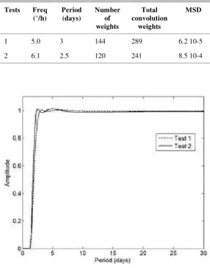
From the analysis of MSD values, the minimum error among overall tests was found under the following conditions: Ω1 of 5°/hour and 144 weights (289 weights convoluted altogether), with MSD of 6.2 10-5 (Table 3). These values agree with the mathematical requirement which defines that the sum of Ω1 and Ω2 may not be multiples of 180º/h and reflect the best adherence of the response function to the filter idealized by Thompson (1983). However, there was another set of values which complied with the aforementioned requirements, with an even smaller number of weights (e.g. 120 weights) and greater proximity between the cut-off frequencies. The goal is to get as close as possible to the ideal filter, i.e. a square wave, which would result in a very small distance between Ω1 and Ω2, such that they would merge into a single frequency. Successive approximations to the Fourier series, and hence to the transfer function, are not convergent near discontinuities. These are explained by a truncation error of the Fourier series when trying to approximate sine and cosine of a real function (Fig. 3).

Table 3. Summary of the highest sets of values to optimize the low-pass filter of Thompson.

Tests Freq (°/h)

Period (days)

Number of weights

Total convolution

weights

MSD

1 5.0 3 144 289 6.2 10-5

2 6.1 2.5 120 241 8.5 10-4

The second set (Test 2) of optimum values ally the lowest MSD and the possible number of weights along the shortest distance between the cut-off frequencies, with no significant disturbance generated by Gibb’s phenomenon.

Since no filter is perfect, as noise from the stop-band cannot be completely removed and certain frequencies in the pass-band will be distorted, it is often necessary to rescale the output series so that the total variance in the pass-band spectral estimates equals the total variance of the input data for that frequency range (EMERY; THOMSON, 2001). In this study, the rescaling process was carried out using a Hanning window. In Figure 3, it can be seen that Test 1 allowed the passage of oscillations of 2.7 days (0.9816) and resulted in the transfer of power in periods of 3.2 days (1.005), 5 days (1.001), 5.5 days (1.012), 6.7 days (1.004) and 7.5 days (1.002). In the second test, oscillations above 2.3 days (0.992) were retained by the filter and there was a power transfer for periods of 2.6 days (1.012), 4.6 days (1.013), 5 days (1.014) and 6 days (1.007). In both tests there was a power transfer to the ‘high’ (order of less than 3 days) and to the ‘low’ (order of 3 days and longer) frequencies, allowing the passage of oscillations between semidiurnal and terdiurnal bands. According to Thompson (1983), some power leakage to higher frequencies is to be expected, since the filter best performs at suppressing tides and is necessarily good at suppressing a particular inertial frequency. In other words, the best filter is the one that transmits less power (THOMPSON, 1983). Emery and Thomson (2001) suggest that the frequency response functions should have reasonably sharp transitions between adjacent stop and pass-bands, especially if the data do not have wide ’spectral-gaps’ between the dominant frequencies of the two bands, as occurs in this study.

The same technique was used to filter out the wind stress components obtained from the Reanalysis project (NCEP/NCAR). However, in this case the filter had to be adapted to a 6 hour-sampling. The filtering of meteorological data should retain the same characteristics as the filter optimized for Cananeia (Test 2), with the same bandwidth and data loss as those of the sea level data. Thus the chosen parameters corresponding to the number of weights and cut-off frequencies are respectively: 21 weights (41 weights convoluted altogether), 1= 36.6°/6 h and 2= 79.2°/6 h.

Power Spectral Density of MSL

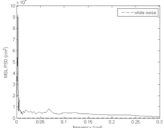
The annual and interannual oscillations represent most of the energy peaks found in the sea level data series. The MSL’s maximum power peak lies in an annual oscillation (0.00269 cpd – period of 372.4 days). Secondary peaks of significant energy

(energy that exceeded the white noise’s threshold) were found at higher frequency bands, with oscillations between 3 to 50 days. The most energetic oscillation among these higher frequencies was represented by the fluctuation with a 50-day period, as can be seen in Figure 4.

Fig. 4. Power spectrum density of MSL from 1955 to 1993 (solid line) and white noise area (dashed line).

Power Spectral Density of Parallel Wind Stress Component (T//)

The spectra obtained for the parallel wind stress component (T//), indicated that the NCEP/NCAR point 1 always had the lowest energy level among all the grid points considered. This may be explained by the non-physical limitations of the NCEP/NCAR model, such as grid resolution, morphological discretization and coastal proximity, which may result in a loss of reliability of the modeled data on these regions. Of the maximum peaks of the spectra analyzed, most occurred at an annual oscillation with a frequency of 0.00269 cpd (period of 371.7days). Another annual fluctuation was captured at a frequency of 0.00256 cpd (period of 390.6 days) at point 2 (Fig. 5A). An interannual oscillation was detected at point 1, with a period of 497.5 days (0.00201 cpd). The most energetic oscillation at point 4 was on a seasonal scale, with a frequency of 0.00549 cpd (period of 182.2 days), that exceeds the energy captured by the annual oscillation at point 3. However, the values of the coherence of this oscillation (seasonal) were less than 50 %, thus contrasting with the high levels of coherence found for annual oscillation (above 70%).

Cross-correlation Between MSL and Parallel Wind Stress Component (T//)

time domain (given in days). The lags with a negative sign were interpreted as indicative of the pause in the action of the wind stress components on MSL or derived from the formation of platform waves that are advanced in time as compared with the evolution of the weather systems (UAISSONE, 2004 apud OLIVEIRA, 2007). The opposite happens when the lags are positive.

The analysis of maximum spectral density lies in the same frequency of 0.00269 cpd in the

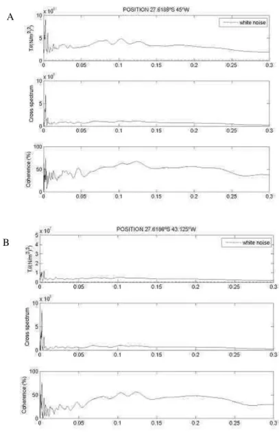
spectra of MSL, in the parallel wind stress component spectra and in cross-spectra analysis. The MSL´s highest energy peak occurred in this frequency, and this was compatible with the T// component and cross-spectral analysis, both in the same period. Points 2 and 4 are those that had, respectively, the highest energy values of T// and MSL versus T//, as can be seen in Figure 5. Regarding the lag, there is a predominance of phases equal to zero, when the atmospheric forcing and the MSL response are in phase.

Figs 5a,b. Spectral analysis of parallel wind stress component (T//) since 1955 to 1993, spatially distributed over four grid points, exemplified by point 2 (as a representative of the points near the coast) and point 4 (as representative of the points far from the coast) : a) point 2; b) point 4. Evaluation of power spectral density, cross spectrum between MSL and T//, coherence, respectively. White noise area was delimited by the dashed line.

A

Power Spectral Density of Perpendicular Wind Stress Component (T|)

In general, the power spectral density of the perpendicular wind stress component had higher values than those estimated for the parallel component at all the points sampled. There is a clear predominance of annual oscillations in the energy domain, such as the frequencies of 0.00275 cpd and 0.00269 cpd, respectively. Sometimes those frequencies could be as much as ten times more energetic that their counterparts in the parallel component analysis (Fig. 6). Those oscillations also sometimes showed higher coherence with MSL, with values above 65%.

Cross-correlation Between MSL and Perpendicular Wind Stress omponent (T|)

The analysis of the perpendicular wind stress component energy and its correlation with the MSL suggested that the maximum values were concentrated in the annual frequency (371.7 days), detected at point 4, as can be seen in Figure 6. This annual fluctuation (0.00269 cpd) was the dominant peak at all the grid points, as was also observed on the MSL spectrum. This oscillation also had high levels of coherence, all above 65% (the maximum being found at point 1 with a value of 75.2%). As for the parallel wind stress component, MSL and perpendicular wind stress component were also in phase.

Figs 6a,b. Spectral analysis of perpendicular wind stress component (T|) from 1955 to 1993, spatially distributed over four grid points, exemplified by point 2 (representating the points near the coast) and point 4 (representing the points further from the coast): a) point 2; b) point 4. Evaluation of power spectral density, cross spectrum between MSL and T|, coherence, respectively. The white noise area has been delimited by the dashed line.

A

D

In both tests involving wind stress components, there was nearly the same variance (≈

26%) as with the original tide gauge series. Thus, it can be stated that the high-frequency oscillations - especially the local tidal harmonic components, are the cause of approximately 75% of the total variance of the series. There was a similar influence of high frequency phenomena on the tide gauge variance in the coastal regions of Rio de Janeiro and at Paranagua, where the proportion was even higher than 88%, as can be seen in Table 1.

In order to ensure that the filters work on the same frequency band for both sea level and wind stress components, the cut-off windows used in this study were chosen based on the analysis of the influence of atmospheric disturbance (wind stress) on the variation of MSL. It was assumed that weather periods longer than 3 days influenced the MSL disturbance over that same period. However, as the atmosphere and the ocean are fluids of different characteristics, which also respond to the influence of similar frequencies, there can be interactions in different periods in response to the same disturbance.

Spectral Analysis

The correlations between MSL and wind stress components for the entire period of 39 years showed that the annual oscillations presented the most energetic peaks, mainly in T| analysis. However the influence of the T// would be a possible explanation for the variation of sea level, since this component was energetic significant, and the T| component had lower coherence than the T//. Thus, an oscillation may not be effective in influencing the sea level variation if it only shows a strong power with MSL (significant peak compared to the spectral range) without having enough coherence.

Regarding the phase signals, oscillations of higher coherence values had null phases, which can be interpreted as indicative of a simultaneous action of wind forcing and MSL. Throughout the 39-year period, energy peaks' influence on annual oscillations tended to decline over the years, and thus their contribution to the variation of MSL in the coastal region of Cananeia was reduced through time. On the other hand, secondary peaks of energy (periods below 50 days) presented increasing trends over the period under analysis.

C

The analysis of Thompson´s low-pass filters resulted in the selection of Test 2, which brought

together the basic assumptions of the optimal filter, i.e.: i) lower MSD and ii) sum of cutoff frequencies different from multiples of 180º/h; iii) the shortest distance between Ω1 and Ω2, and iv) with no significant disturbance by Gibb's phenomenon.

The spectra were analyzed within a restricted frequency band of periods longer than 3 days, or 0.33 cpd. However there was a mathematical leakage of energy outside the spectral range chosen. In other words, a part of the ‘high’ frequencies (periods of less than 3 days) were not ideally attenuated by the low pass Thompson filter. Despite that, these inconsistencies were below 10% of the average PSD peaks found in the entire spectrum. This was then considered a noise and thus incorporated into the study, since the filtering was considered successful, although not perfect.

In general the spectra presented power peaks over the years analyzed, which suggested the prevalence of phenomena caused by the influence of wind stress, being mainly associated with annual oscillations (mainly the oscillation with periods of 0.00269 cpd). They also combined energy peaks with the highest coherence values found in the overall analysis, as they were responsible for the largest MSL variance in the coastal region of Cananeia.

Oscillations of shorter period with coherence values above 70% also stood out. However, these oscillations were not associated with a significant energy level. Higher coherence frequencies were not necessarily associated with maximum peaks of energy. The sample points obtained from the grid of the NCEP/NCAR global model presented different responses to the disturbance during the same period, indicating that the disposition of these points in some way affected the detection of similar spectral bands. Non-physical limitations of the NCEP/NCAR model, such as grid resolution and morphological discretization may have introduced some restrictions to the estimated results. Point 1 always presented the lowest energy level in relation to other sampling points, possibly due to its proximity to the continent. Grid points closer to the coast may have been biased by the global model resolution, which probably did not distinguish the influence of the continent, resulting in the loss of reliability of modeled data. The opposite occurred at point 4 (the grid point furthest offshore in this study), which showed more robust results. The offshore points, i.e. 2 and 4, were those with the higher frequencies of coherence and energy throughout the study.

It is concluded that the wind stress components can affect not only the MSL variation through oscillations with periods of the order of days, associated with the passage of cold fronts (periods of 3 to 10 days) or on storm surge-scales (i.e. 3 to 30 days) – as described by Uaissone (2004 apud Oliveira, 2007), Castro et al. (2006) and Pugh (1996), but also through annual and interannual oscillations. The parallel component of the wind stress seems to be more effective in the region of Cananeia than the perpendicular component, mainly due the association of high coherence and energy peaks.

The inclusion of sea level atmospheric pressure is recommended as a parameter to improve the understanding of frontal systems' effects on MSL variations and on wind stress components, as well as the future projection of the main oscillations found in the coastal region of Cananeia (SP) as a result of climate change scenarios.

A

The authors thank Prof. Claudio Neves (COPPE-UFRJ) for his invaluable assistance in preparing this study and CAPES for the financial support granted to the first author.

R

CAMARGO, R.; HARARI, J. Modelagem numérica de ressacas na plataforma sudeste do Brasil a partir de cartas sinóticas de pressão atmosférica na superfície. Bol. Inst. Oceanogr., v. 42, n. 1/2, p. 19-34, 1994.

CAMARGO, R.; HARARI, J.; CARUZZO, A. Numerical modeling of tidal circulation in coastal areas of the southern Brazil. Afro-Am. Gloss News.,v. 3, n. 1, 1998. CAMARGO, R.; HARARI, J.; CARUZZO, A. Basic statistics of storm surges over the south-western Atlantic. Afro-Am. Gloss News., ed. 3, n. 2, 1999.

CASTRO, B. M.; LORENZZETTI, J. A.; SILVEIRA, I. C. A.; MIRANDA, L. B. Estrutura termohalina e circulação na região entre Cabo de São Tomé (RJ) e o Chuí (RS). In: ROSSI-WONGTSCHOWSKI, C. L. B.; MADUREIRA, L. S. P. (Org.). O ambiente oceanográfico da Plataforma Continental e do Talude na região sudeste-sul do Brasil. São Paulo: EDUSP, São Paulo, 2006. 472 p.

COSTA, M. C.; BERNARDES, M. E. C. Estimativa do Nível Médio do Mar (NMM) em Cananéia (SP) a partir da otimização do Filtro de Thompson. In: CONGRESSO BRASILEIRO DE OCEANOGRAFIA, 4., 2010, Rio Grande, RS. Anais ... Trabalho n. 1019, p. 01943-01945. CD Rom.

DUCHON, C. E. Lanczos Filtering in one and two dimensions. J. Appl.Meteorol., v. 18, p. 1016-1022, 1979.

EMERY, W. J.; THOMSON, R. E. Data analysis methods in Physical Oceanography. Amsterdam: Elsevier Science , 2001. 636 p.

FRANCO, A. S. Análise espectral contínua e discreta. São Paulo: Instituto de Pesquisas Tecnológicas do Estado de São Paulo, 1982. 194 p.

FRANCO, A. S.; ROCK, N. J. The fast Fourier transform and its application to tidal oscillation. Bol. Inst. Oceanogr., 1971.

HARARI, J.; CAMARGO, R. Simulação da propagação das nove principais componentes de maré na plataforma sudeste brasileira através de modelo numérico hidrodinâmico. Bol. Inst. Oceanogr., v. 42, n.1, p. 35-54,1994.

HARARI, J.; CAMARGO, R. Tides and mean sea level variabilities in Santos (SP), 1944 to 1989. Relatório Interno Inst. Oceanogr., n. 36, p. 1-15, 1995.

HARARI, J.; FRANÇA, C. A. S.; CAMARGO, R. Variabilidade de longo termo de componentes de marés e do nível médio do mar na costa brasileira. Afro-Am. Gloss News, ed. 8, n. 1, 2004.

KALNAY, E.; KANAMITSU. M.; KISTLER, R.; COLLINS, W.; DEAVEN, D.; GANDIN, L.; IREDELL, M.; SAHA, S.; WHITE, G.; WOOLLEN, J.; ZHU, Y.; LEETMAA, A.; REYNOLDS, R.; CHELLIAH, M.; EBISUZAKI, W.; HIGGINS, W.; JANOWIAK, J.; MO, K. C.; ROPELEWSKI, C.; WANG, J.; JENNE, R.; JOSEPH, D. The NCEP/NCAR 40-Year Reanalysis Project. In: Bull. Am. Meteor. Soc., Mar. 1996.

KUMARESAN, R. Spectral analysis. In: MIRTA, S. K.; KAISER, J. F. (Org.). Handbook for digital signal processing. New York: John Wiley & Sons, 1993. p. 1143 – 1237.

MESQUITA, A. R. Marés, circulação e nível do mar na costa sudeste do Brasil. Documento preparado à Fundespa (Fundação de Estudo e Pesquisas Aquáticas) 1997. Disponível em: <www.fundespa.com.br>. Access: 01 Sep. 2009.

MESQUITA, A. R. Sea level variations along the brazilian coast: a short review. In: BRAZILIAN SYMPOSIUM ON SANDY BEACHES, 2000, Itajaí, SC. Anais… Itajaí: 2000.

MESQUITA, A. R. Hourly, daily, seasonal and long-term sea levels along brazilian coast. Afro-Am. Gloss News, jan. 2002.

MESQUITA, A. R. O gigante em movimento. Scientific American Brasil, v. 1, p. 17-23, 2009. (Especial Oceanos)

MUNK, W. Twentieth century sea level: An enigma. P. Natl Acad.Sci. USA, v. 99, n. 10, p. 6550-6555, 2002. NEVES, C. F.; O nível do mar: uma realidade física ou um

critério de engenharia? Vetor, v. 15, n. 2, p. 19-33, 2005. NEVES, C. F.; MUEHE, D. Vulnerabilidade, impactos e adaptação a mudanças do clima: a zona costeira. In: Mudança do clima no Brasil: vulnerabilidade, impactos e adaptação. Brasília, DF.: Centro de Gestão e Estudos Estratégicos, n. 27, 2008. p. 217-297. (Série Parcerias Estratégicas).

NOAA, Mean sea level trend 874-051 Cananeia,

Brazil. Disponível em: <

http://tidesandcurrents.noaa.gov/sltrends/sltrends_global _station.shtml?stnid=874-051>. 17/8/2012

OLIVEIRA, M. M. F.; EBECKEN, N. F. F.; OLIVEIRA, J. L. F.; SANTOS, I. A. Neural Network Model to predict a storm surge. J. Appl. Meteor. Clim., v. 48, p. 143-155, 2009.

PAWLOWICZ, R.; BEARDSLEY, B.; LENTZ, S. Classical tidal harmonic analysis including error estimates in MATLAB using T_TIDE. Comput.Geosci., v. 28, p. 929-937, 2002.

PICARELLI, S. S.; HARARI, J.; CAMARGO, R. Modelling the tidal circulation in Cananeia-Iguape estuary and adjacent coastal area (São Paulo, Brazil). Afro- Am. Gloss News, ed. 6, 2002.

PUGH, D. T. Tides, surges and Mean Sea-Level. Swindon: John Wiley & Sons, 1996. 486 p.

THOMPSON, R. O. R. Y. Low-pass filters to supress inertial and tidal frequencies. J. Phys. Oceanogr., v. 13, p.1077-1083,1983.

(Manuscript received 28 July 2011; revised 14 July 2012; accepted 24 July 2012)