Table 1 : Differintegration in context of Laplace transform

Introduction

t o

fractional linear

systems.

Part

1

:

zyxwvutsrqponmlkjihgfedcbaZYXWVUTSRQPONMLKJIHGFEDCBA

Continuous-time

case

M.D.Ortigueira

zyxwvutsrqponmlkjihgfedcbaZYXWVUTSRQPONMLKJIHGFEDCBA

Abstract:

zyxwvutsrqponmlkjihgfedcbaZYXWVUTSRQPONMLKJIHGFEDCBA

In the paper, the class of continuous-time linear systems is enlarged with the inclusion

of fractional linear systems. These are systems described by fractional differential equations. It is shown how to compute the impulse, step, and frequency responses from the transfer function. The theory is supported by definitions of fractional derivative and integral, generalisations of the usual. An introduction to fractal signals as outputs of fractional differintegrators is presented. It is shown how to define a stationary fractal.

1 Introduction

Fractional calculus is nearly 300 years old. In fact, in a letter to Leibnitz, Bernoulli put him a question about the meaning of a non-integer derivative order. It was the beginning of a discussion on the theme that involved other mathematicians such as L‘ Hhpital, Euler and Fourier

[ 1-31, However we can trace the beginning of the fractional calculus in the works of Liouville and Abel. Abel solved an integral equation representing an operation of fractional integration. Liouville made several attempts and presented a formula for fractional integration

where T(p) is the gamma function. With the term ( - 1)p omitted, we call this the Liouville fractional integral. Liouville developed ideas on this theme and presented a generalisation of the notion of incremental ratio to define a fractional derivative. This idea was discussed again by Grunwald (1867) and Letnikov (1 868). Riemann reached an expression similar to eqn. 1 for the fractional integral.

Holmgren (1 86Y66 and Letnikov 1868/74) discussed this problem when looking for the solution of differential equations, putting in a correct statement thc fractional differentiation as inverse operation of the fractional inte- gration. Hadamard proposed a method of fractional differ- entiation based on the differentiation of the Taylor’s series associated with the function. Weyl (1917) defined a frac- tional integration suitable to periodic functions, and Marchaud (1 927) presented a form of differentiation based on finite differences. More recently, the unified formulation of integration and differentiation (differ- integration) based on Cauchy’s integral [4-61 has gained

great popularity.

zyxwvutsrqponmlkjihgfedcbaZYXWVUTSRQPONMLKJIHGFEDCBA

C IEE 2000

IEE Proceedings online no. 20000272 DOI: 10.1049/ip-vis:20000272

Paper received 9th September 1999

The author is with the lnstituto Superior Tecnico and UNINOVA, Ca~npus

da FCT da

zyxwvutsrqponmlkjihgfedcbaZYXWVUTSRQPONMLKJIHGFEDCBA

UNL, Quinta da Tort-e 2825 - 114 Monte da Caparica, Portugal

and also with INESC, K. Alves Redol, 9, 2 , 1000 Lisbon, Portugal 62

Applications to physics and engineering are not recent: application to viscosity dates back to the 1930s [7]. The work of Mandelbrot [8, 91 in the field of fractals had great influence and attracted attention to fractional calculus. During the last 20 years, application domains of fractional calculus have increased significantly: seismic analysis [7], dynamics of motor and premotor neurones of the oculo- motor systems [ l o ] , viscous damping [ 1 1 , 121, electric fractal networks [13], l/f noise [14, 151: fractional order sinusoidal oscillators [ 161, and, more recently, control [ 17- 191 and robotics [20]. However, there is no publication with a coherent presentation of fractional linear system theory. Most elementary books on signals and systems consider only the integer derivative order case and treat the corresponding systems, studying their impulse, stcp and frequency responses and their transfer function. It is not such a simple matter, if one substitutes fractional deriva- tives for the common derivatives.

The objective of this paper is to treat the fractional continuous-time linear system as is done with usual systems. Attempts have been made to create a formal framework for the study of fractional linear systems, but without the desired generality, coherence and usefulness of the final results [2, 1 1 , 21-23]. To our knowledge, the approach we propose here is original, although it has an ‘already seen’ character. This is because we are dealing with very well known concepts. We merely generalise them to the fractional case.

We intend to make a first contribution for a correct understanding of some experimental results [ 14, 22, 231 and to create a new way into modelling, simulation, and estimation in real fractional systems.

To begin a study of fractional systems, we need to define fractional derivative. The most obvious approach to the fractional derivative is the Griinwald-Letnikov method, a generalisation of the usual definition based on the incre- mental ratio [ 1-31. However, it is very hard to manipulate and obtain new results. This motivates us to adopt a definition based on the Laplace transforms.

Consider first the Laplace transform (LT) case. Essen-

tially, we are looking for the Laplace inverse transform of

zyxwvutsrqponmlkjihgfedcbaZYXWVUTSRQPONMLKJIHGFEDCBA

3, d(’)(t), with 2 being any positive real number. General-

ising the well known property of the Laplace transform, the

convolution of a Laplace transformable signal

zyxwvutsrqponmlkjihgfedcbaZYXWVUTSRQPONMLKJIHGFEDCBA

.Y( t ) with a(’)(t) has s’X(s) as the LT and is defined as the 2 order

derivative of x(t). If r < 0, the definition remains valid and

we are performing a (fractional) integration. For this

zyxwvutsrqponmlkjihgfedcbaZYXWVUTSRQPONMLKJIHGFEDCBA

reason, we assume

zyxwvutsrqponmlkjihgfedcbaZYXWVUTSRQPONMLKJIHGFEDCBA

c! to be any real and speak of 'differ- integration' (3, 5, 241. As in the integer case, there arc two

functions with

zyxwvutsrqponmlkjihgfedcbaZYXWVUTSRQPONMLKJIHGFEDCBA

s" as the LT, corresponding to the causal and anti-causal cases. The combination of these two allows us

to obtain a definition of differintegration for bilateral signals with a Fourier transform (FT).

The results obtained with the LT are suitable for dealing with linear systems described by fractional linear differ- ential equations. We define transfer function and impulse response in a very similar way to that normally used. We also make a brief study of the stability problem.

We present the definition of differintegration that we have adopted. Interesting topics arc studied: differintegra- tion of periodic functions, the unilateral Laplace transform and the initial conditions, and differintegration of the causal exponential. These results are fundamental to our study of the linear fractional continuous systems. We consider systems defined by fractional differential equa- tions that are uscd to obtain the transfer function and the impulse response. This is obtained by partial fraction expansion. Examples are presented and the problem of the stability is treated briefly. We also consider the state variable formulation.

We study the stochastic processes output of the differ- integrator when the input is white noise. We define a stationary fractional stochastic process, the hyperbolic noise. It is shown that this process belongs to the class of the so-called ' l / f noise', and we obtain a generalisation of the Brownian motion. We also show why some attempts to define a stationary fractal have failed.

Note that in the following and othcrwise stated, we assume to be in the context of the generalised functions (distributions). We always assume that they are either of

cxponential order or tempered distributions.

zyxwvutsrqponmlkjihgfedcbaZYXWVUTSRQPONMLKJIHGFEDCBA

2 Fractional differintegration of continuous-time

signals

2.7 Definition

The simplest way of defining fractional derivative is through the generalisation of the incremental ratio. It is called the Cirunwald-Letnikov approach [3]. However, this approach is not suitable for the application we have in mind, since it is hard to manipulate. Thercfore, wc pursue a different method.

Instead of beginning by a definition of differintegration, let us invert the problem and take the LT as the starting point, not only for thc differentiation, but also for integra-

tion

zyxwvutsrqponmlkjihgfedcbaZYXWVUTSRQPONMLKJIHGFEDCBA

- differintegration. Essentially, we intend to prolong

the sequence

. , s-*,

zyxwvutsrqponmlkjihgfedcbaZYXWVUTSRQPONMLKJIHGFEDCBA

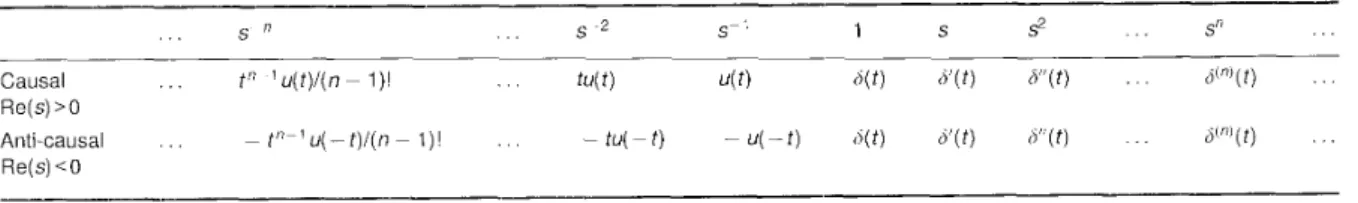
.SF', 1, .si, s 2 , . . . , S n .

zyxwvutsrqponmlkjihgfedcbaZYXWVUTSRQPONMLKJIHGFEDCBA

. . ₍₂₎

in order to include other kinds of exponents: rational or, generally, real (or even complex numbers). It is clear that there are two forms of obtaining the extension, depending on the choice for the region of convergence for the LT: the left and right half-planes. Let us begin by considering both

cases with integer powers and obtaining the corresponding inverses. With these cases, we can form Table 1, where S ( t )

is the Dirac impulse and u ( t ) is the Heaviside unit step function.

To obtain a differintegration of a given function, we only have to convolve it with one of the functions presented in each row. Generalising the notation used for the usual derivatives, we denote by (5( "'(t) the nth order primitive of

S(t). This corresponds to saying that a differintegration of order n (integcr) is given by

.f""'(t) =

.IR,

,f(~)d'*'(t

- ?)dz (3)

zyxwvutsrqponmlkjihgfedcbaZYXWVUTSRQPONMLKJIHGFEDCBA

where 6 ( " ) ( t ) is given in the causal case by

the nth order derivative of 6 ( t ) if n > 0

i I . p

if

zyxwvutsrqponmlkjihgfedcbaZYXWVUTSRQPONMLKJIHGFEDCBA

IZ < 0

P ( t ) = t - ' l - l u ( t )

(4) To define a fractional differintegration, we have to general- ise eqn. 2 to eqn. 4 for non-integer orders. Thus, we have to give a precise meaning to (Si")(t) = LT-' [s']. Note that, in

the general case, a =

1x1

zyxwvutsrqponmlkjihgfedcbaZYXWVUTSRQPONMLKJIHGFEDCBA

+

v

(0

I 1' < l), and so we only have to consider the case 0 < 131 < 1, since

represents the

x

differintegrated of the Dirac's distribution

S T = ,Iv1 + " ._ --s tzl .s', 1 giving the following (6(')(t) always

zyxwvutsrqponmlkjihgfedcbaZYXWVUTSRQPONMLKJIHGFEDCBA

6( t ) ) :

( 5 )

= (pvi)(t)$l,)(t)

The solution for the problem is given by [2, 31 for the causal case. It is a simple task to show that

( 7 )

is the solution for the anti-causal case.

r(t)

is the Euler gamma function [ 3 ] . Returning to eqns. 6 and 7, if

x

> 0, it is a derivation; if

x

< 0, it is an integration. Essentially, eqns. 6 and 7 lead to the Riemann-Liouville and Weyl differintegration schemes, respectively [2, 31.

In the following, we consider the causal case and use the notation D"x(t) =,d")(t), where x(t) is an exponential order signal with X ( s ) as the LT. The differintegration enjoys some interesting properties [2-61, we present three of them.

If x = - [j, we conclude that the fractional differentiation and the fractional integration are inverse operations, as expected.

Table 1 : Differintegration in context of Laplace transform

. . . s " , . . s 2 5-' 1 S 52 . . . s" . . .

Causal . . . t" ' u ( t ) / ( n - I ) ! . . . t 4 t ) u ( t ) 6 ( t ) H'(t) 6"(t) . . . c P ) ( t ) . . .

Re(s) > 0 Re(s)<O

Anti-causal . . . - t " - ' u ( - t ) / ( n - I ) ! . . . - t u ( - t ) - U ( - t ) 6 ( t ) 6 ' ( t ) 6"(t) . . . 6("'(t) . . .

2.1.2 Differintegration in the transform domain:

zyxwvutsrqponmlkjihgfedcbaZYXWVUTSRQPONMLKJIHGFEDCBA

LT[t'x(t)z@)] =

zyxwvutsrqponmlkjihgfedcbaZYXWVUTSRQPONMLKJIHGFEDCBA

(- 1)%(')(3)

zyxwvutsrqponmlkjihgfedcbaZYXWVUTSRQPONMLKJIHGFEDCBA

(9) with

(10) This is similar to the differintegration formula used by Campos [4, 51 and Nishimoto [6], and is a generalisation of the well known Cauchy formula.

2.1.3 Differintegration of the product of

two

func- tions:

This is the Leibnitz' formula for the differintegration of the product. The binomial coefficients ( d k ) are given by where = u(a

+

] ) ( a

+

2) . . . ( a

+

k - 1 j is the Poch- hammer's symbol.

Although in the deductions of the previous results we used the LT, its validity is wider, allowing their use with other functions, as is the case of the exponential defined for all the time. Since we have in mind the study of causal linear systems, we are going to consider mainly the definition introduced in eqn. 6.

Till now, we considered a differintegration of signals with the LT that exclude, for example, the sinusoids defined for all the time and other similar signals with a Fourier transform, but not the Laplace transform (or its region of convergence is degenerate). This means that we

look for a sequence like that presented in eqn.

zyxwvutsrqponmlkjihgfedcbaZYXWVUTSRQPONMLKJIHGFEDCBA

2 but with

Jw instead of s. We must begin by noting that the FT of the signum function, sgn(t), is given by 2/jto. With this, we can present Table 2.

Table 2 suggests the introduction of the following definition of differintegration of d ( t ) :

This can be considered as the arithmetic mean of causal and anti-causal differintegrations, if we extend their regions of convergence to include the imaginary axis. This is the Rieman-Hilbert problem: to define a function on the boundary of the analyticity regions of two functions. We have

2

.

A(w)

zyxwvutsrqponmlkjihgfedcbaZYXWVUTSRQPONMLKJIHGFEDCBA

= 2 . FT[Gr'(t)]

= F T [ 4 ? ( t ) ]

+

FT[5(Y)(t)]

= lim

zyxwvutsrqponmlkjihgfedcbaZYXWVUTSRQPONMLKJIHGFEDCBA

s2

+

lim s' (14)

S€C'+JO d " + J ' O

where C" and

zyxwvutsrqponmlkjihgfedcbaZYXWVUTSRQPONMLKJIHGFEDCBA

d

represent the right and left half complex planes. This immediately gives A(w) = ( j w ) " .

zyxwvutsrqponmlkjihgfedcbaZYXWVUTSRQPONMLKJIHGFEDCBA

Table 2: Differintegration in context of Fourier transform

Before finishing here, we must consider the application fields of the second approach. It is not hard to see that if the function has the LT convergent in a strip that includes the imaginary axis, both definitions give the same result. If the strip degenerates in the imaginary axis, as is the case of many bilateral signals, the function has the FT (at least in the generalised sense) and we must use eqn. 12. Of course, in applications to the study of causal systems, we must use the approach based on the LT.

2.2 Differin tegra tion of periodic functions

Now we have the problem of the differintegration of a periodic function, x/>(rj, These functions do not have the LT, but they have the FT. A given periodic function, with

period T, can be considered as a sum of delayed versions of

a

given basic wavelet. Mathematically, we have leading to

This shows that the differintegrator of a periodic function can be obtained by convolving the wavelet with the differintegrator of the comb signal. To obtain the corre- sponding Fourier series, we must find the differintegration of the exponential eJ"'Or for all t E R. The FT of this function

is 27c6(0 - wo). This leads us to conclude that its

zyxwvutsrqponmlkjihgfedcbaZYXWVUTSRQPONMLKJIHGFEDCBA

2 order

fractional differintegrator is the inverse FT of

2n.

(@)' .

6(w - coo) = 271. (jcoO)' .6(co - too). The inverse of this transform is

Using the FT in eqn. 16, we have

If

c% < 0, we must assume a zero mean value periodic function X ( 0 ) = O . Inverting the FT and putting

oo

=

2 d T , we obtain

2.3 Unilateral Laplace transform and initial

conditions

zyxwvutsrqponmlkjihgfedcbaZYXWVUTSRQPONMLKJIHGFEDCBA

The solution of fractional differential equations can be done using the unilateral LT. As in the ordinary equations, this transform introduces the initial conditions naturally. For this, we need a generalisation of the usual theorem of

the LT of the derivative. Let x ( t ) be a signal and

zyxwvutsrqponmlkjihgfedcbaZYXWVUTSRQPONMLKJIHGFEDCBA

X ( s ) its unilateral LT. It is known that

n-l

LTIDflx(t)] =

zyxwvutsrqponmlkjihgfedcbaZYXWVUTSRQPONMLKJIHGFEDCBA

S X ( S ) - s"-'-'x(')(o) (20)

/=U

To generalise this result, for any order c( >

0,

let m be the

least natural number greater than or equal to a : m

zyxwvutsrqponmlkjihgfedcbaZYXWVUTSRQPONMLKJIHGFEDCBA

2

2.

zyxwvutsrqponmlkjihgfedcbaZYXWVUTSRQPONMLKJIHGFEDCBA

D-("'-') then corresponds to integration and multiplication by s ~ ( ~ - ' ) in the transformed domain. We have succes- sively [3]

L T [ D " ~ ( t ) ] = L T [ D ~ ~ [D-(" -?Ix(

zyxwvutsrqponmlkjihgfedcbaZYXWVUTSRQPONMLKJIHGFEDCBA

t ) ] ] = . y n 7 ~

zyxwvutsrqponmlkjihgfedcbaZYXWVUTSRQPONMLKJIHGFEDCBA

T [ D - ( " - ~ ) ~ ( t)]

n7- I

which is the desired result (this can also be obtained from eqn. 11, by putting y ( t ) = ~ ( t ) . ) With this result, we can deduce generalisations of the initial and final value theo- rems. For the former, we obtain

For the final value, we have

x ~ ~ ' ) ( c o ) = lims"X(s) Re(s) _\+0 > 0 (23) The proofs are very similar to the usual, and so we do not present them.

2.4 Differintegration of the causal exponential

This case is exceptionally important, since it appears in the computation of the impulse and step responses of linear causal systems. We do not consider the case of integer

differintegration. Here, we have

zyxwvutsrqponmlkjihgfedcbaZYXWVUTSRQPONMLKJIHGFEDCBA

1 P t

We represent this function by E,(t,a), with Eo(t,a) = e'"u(t) and E,(t,O) = cZ('-')(t). The study of this function is normally done in terms of the incomplete gamma function

[ 1, 21. Here, we use the power series approach.

The generalised Leibnitz' rule allows us to obtain

directly a power series for E,(t,a). We only have to make

zyxwvutsrqponmlkjihgfedcbaZYXWVUTSRQPONMLKJIHGFEDCBA

x ( t ) = u ( t ) and y(t)=e'' in eqn. 1 I . As u@)(t)=

d("-l)(/) = t-"/T(l - a), (another power series for this function is presented elsewhere [ 2 ] ) then,

This gives, after some manipulation

This equation shows that all the non-integer derivatives of the causal exponential are not continuous at the origin and go to infinity. This has important implications in applica- tions to linear systems. The LT of this function is easily obtained, following the theory developed in Section 2.2,

and is

zyxwvutsrqponmlkjihgfedcbaZYXWVUTSRQPONMLKJIHGFEDCBA

S

'

LT[E,(t, U ) ] = ~ Re(s) > Re(a) (27)

As Re(s) > Re(a), we can always work in the region

Is1 > IuI, and so eqn. 27 can be written

s -

a

+m

LT[E,(t, a)] = a n S x - n - l Is1 > IUI (28)

0

This expresses a special case of the more general result known as Hardy's theorem [ 2 5 ] :

Let the series

0

be convergent for some Re(s) > so > 0 and

zyxwvutsrqponmlkjihgfedcbaZYXWVUTSRQPONMLKJIHGFEDCBA

CI > ~ 1. The

series

+m

,f(t) = U,f+'l

0

converges for all t > 0 and F ( s ) = Lm(t)].

3 Fractional continuous-time linear systems

3. I Description

The most common and useful continuous-time linear systems are the lumped parameter systems, described by linear differential equations. The simplest of these systems are the integrators, differentiators and constant multipliers (amplifiers/attenuators). The referred lumped parameter linear systems are associations (cascade, parallel or feed- back) of those simple systems. Here, we study the systems that result from the use of fractional differentiators or integrators, and that are described by linear fractional differential equations. We assume that the coefficients of the equation are constant, and so the corresponding system is a fractional linear time-invariant (FLTI) system. With this definition, we are ready to define and compute the impulse response and transfer function.

We therefore consider FLTI systems described by a differential equation with the general format

N M

n=O m=O

where D is the derivation operator and v,, are the orders of differintegration that, in the general case, are complex numbers. Here, we assume they are positive real numbers.

As usual, we apply the

LT

to eqn. 3 1, obtaining easily rw

bPls'','~

a n s ' ~ ~

IV (32)

H ( s ) = m=O

,,=0

which is the transfer function, provided that Re(s)

zyxwvutsrqponmlkjihgfedcbaZYXWVUTSRQPONMLKJIHGFEDCBA

> 0 or Re(s) < 0. If we use the FT instead of the LT, we would

obtain the frequency response,

zyxwvutsrqponmlkjihgfedcbaZYXWVUTSRQPONMLKJIHGFEDCBA

H o w ) , and could represent the Bode diagrams as in usual systems. It is interesting to

note that the asymptotic amplitude Bode diagrams consti- tute straight lines with slopes that, at least in principle, may assume any value; this is in contrast to the usual case, where the slopes are multiples of 20 dBidecade. To obtain the frequency response directly from eqn. 32, we must proceed as in Section 2.1. The result would be that

achieved by letting s go t o j o in eqn. 32

zyxwvutsrqponmlkjihgfedcbaZYXWVUTSRQPONMLKJIHGFEDCBA

3.2 From the transfer function to the impulse response

To obtain the impulse response from the transfer function, we proceed almost as usual. However, we must be careful. Let us begin by considering the simple case of a differ- integrator:

H ( s ) = s7

zyxwvutsrqponmlkjihgfedcbaZYXWVUTSRQPONMLKJIHGFEDCBA

9! f 0 ( 3 3 )

s’ is a multi-valued expression defining an infinite number of Riemann surfaces. Each Riemann surface defines one function. Therefore, eqn. 33 can represent an infinite number of linear systems. However, only the principal

Riemann surface

zyxwvutsrqponmlkjihgfedcbaZYXWVUTSRQPONMLKJIHGFEDCBA

{z: - n 5 arg(z) < n} may lead to a real system. Constraining this function by imposing a region of

convergence, we define a transfer function. Eqn. 6 or 7 gives the corresponding impulse response.

Now, go a step further and consider the simple case corresponding to the fraction

where v is a real number. The equation

zyxwvutsrqponmlkjihgfedcbaZYXWVUTSRQPONMLKJIHGFEDCBA

s“ = a has infinite solutions on a circle of radius Ial””. However, in the

general case, we cannot ensure the existence of one pole in the principal Riemann surface. This is not the case for 0 <

v

5 1. In this case, we may have one pole on that branch. For this reason, we focus on the following cases:

(a) v, are rational numbers that we write in the form plt/q,l.

Let q be the least common multiple of the q,; then = n/q,

where n and q are positive integer numbers. So, v n = n . i’,

with v = liq (a differential equation with

zyxwvutsrqponmlkjihgfedcbaZYXWVUTSRQPONMLKJIHGFEDCBA

v = 112 is semi- differential [28]). The coefficients and orders do not coin-

cide necessarily with the previous ones, since some of the coefficients can be zero: for example

[ad/’

+

hD’/2]y(t) = x(t)

[ h ~ ’ . l / 6 + . ~ 2 , 1 / 6

+

0 ‘ D 1 / 6 ] y ( t ) = x ( t )

transforms into:

( 3 5 )

(6) \I,~ are irrational numbers but multiples of CI

zyxwvutsrqponmlkjihgfedcbaZYXWVUTSRQPONMLKJIHGFEDCBA

(0 4

Eqns. 31 and 32 then assume the general forms

< 1) Y L1

11=0 m=O

and

With a transfer function as in eqn. 37 we can perform the inversion quite easily, by following the steps below: (i) transform H ( s ) into H ( z ) , by substitution of s’ for z [we are assuming that H ( z ) is a proper fraction; otherwise, we have to decompose it in a sum of a polynomial (inverted separately) and a proper fraction.]

(ii) the denominator polynomial in H ( z ) is the indicial polynomial [3] or characteristic pseudo-polynomial [ 181; perform the expansion of H ( z ) in partial fractions (we must use only the zeros of the indicial polynomials that are really in the principal Riemann surface.)

(iii) substitute back si’ for z, to obtain the partial fractions i n the form

( 3 8 )

1

F ( s ) = ~ k = 1 , 2 . . . .

(9 - L$

zyxwvutsrqponmlkjihgfedcbaZYXWVUTSRQPONMLKJIHGFEDCBA

(iv) invert each partial fraction.

(v) add the different partial impulse responses.

3.3 Partial fraction inversion

3.3.1 Rational case: We proceed to the inversion of

the partial fraction (eqn. 38), considering first the k = 1 and

zyxwvutsrqponmlkjihgfedcbaZYXWVUTSRQPONMLKJIHGFEDCBA

TI = l i q case. Using the well known result referring the sum

of the first q terms of a geometric sequence, we obtain because r = bls, we obtain

y

= (1 - h ) . b1-I . .$-J

j = 1

q

1

hJ- 1 , ,YVi 1 i=l

- from where ~ -

I - h ,Y? - h‘l

(40) We conclude that the LT inverse of a partial fraction as

F ( s ) = l/s’/q - n is a linear combination of q fractional derivatives of EO(t,aq) =e“““. U ( / ) :

The k > 1 case in eqn. 38 does not present great difficulties, except some additional work. We can use eqn. 39 repeat- edly and the convolution to solve the problem. Alterna- tively, we can differentiate. For example

withj(t) given by eqn. 4 1. We do not proceed further, since this example shows how we can proceed in the general case.

IEE P I U C . - V ~ ~ . l r n ~ g e S i p ~ l PI.OC~.S\.,

zyxwvutsrqponmlkjihgfedcbaZYXWVUTSRQPONMLKJIHGFEDCBA

I61 147, i\‘a I , Fehrltcq 2000

3.3.2 Irrational case:

zyxwvutsrqponmlkjihgfedcbaZYXWVUTSRQPONMLKJIHGFEDCBA

Consider now the case corre-

sponding to

zyxwvutsrqponmlkjihgfedcbaZYXWVUTSRQPONMLKJIHGFEDCBA

11 an irrational number, 0

zyxwvutsrqponmlkjihgfedcbaZYXWVUTSRQPONMLKJIHGFEDCBA

< v < 1. To invert

eqn. 38 when 11 is irrational, we can use a known result [4]:

the LT of the Mittag-Leffler function

(44) is given by

s'-l

Y ( S ) = ~ Re(s) > 1 (45)

zyxwvutsrqponmlkjihgfedcbaZYXWVUTSRQPONMLKJIHGFEDCBA

S'' - 1 '

Therefore, in terms of this function, it is not hard to conclude that F(s) is the LT of the ( 1 - v)th order deriva- tive of the function i//(at')

f(t) = D ' p " [ ~ b ( ~ t l ' ) ] (46) The Mittag-Leffler function can be considered as a general- isation of the exponential with which it coincides when

v = 1. Eqn. 4 1 (and eqn. 45) suggests that we work with the step response instead of the impulse response, to avoid derivatives or working with non-regular functions near the origin.

3.4 Stability of FLTI continuous-time systems

Our study of the stability of the FLTI systems is based on the B I B 0 (bound input, bound output) stability criterion, which implies stability when the impulse response is absolutely integrable.

The simplest FLTI system is the system with transfer

function

zyxwvutsrqponmlkjihgfedcbaZYXWVUTSRQPONMLKJIHGFEDCBA

H ( s ) = s " , where s belongs to the principal

Riemann surface. If

zyxwvutsrqponmlkjihgfedcbaZYXWVUTSRQPONMLKJIHGFEDCBA

v > 0, the system is definitely unstable, since the impulse response is not absolutely integrable,

even in a finite interval. If - 1 < 11 < 0, the impulse

response remains a limited function when t increases indefinitely and it is absolutely integrable in every finite interval. Therefore, we say that the system is wide-sense stable. This case is interesting to the study of the fractional stochastic processes. If v = - 1, the normal integrator, the system is wide-sense stable. The case v < - 1 corresponds to an unstable system, since the impulse response is not a

limited function when t goes to

+

00.

zyxwvutsrqponmlkjihgfedcbaZYXWVUTSRQPONMLKJIHGFEDCBA

These considerations tell us that a system with poly- nomial transfer function

P K ( s V )

= CEO u,s"~ is stable if

l K .

V I

< 1. Thus, in the case of a pole-zero system, with N poles, the number of zeros must be less than

N+

l/v. Consider the LTI systems with transfer function H(s) a

quotient of two polynomials in s'. Let us go back to the partial fraction (eqn. 38) with v = l / y and k = 1, which was transformed into eqn. 39. The poles are therefore integer

powers of complex numbers. The transformation w = z'

zyxwvutsrqponmlkjihgfedcbaZYXWVUTSRQPONMLKJIHGFEDCBA

[ transforms the sector 0 5

H

5 271/q(O = arg(z)) into the

entire complex plane. The sector 71/24

5

H 5 71/24

+

z/q is then transformed in the left half-plane [36]. It is not difficult to show that the same happens to the sectors obtained by rotating the previous one by an angle i ' 2 d q

(i = 1 , . . . , q - 1). Then, if we let H be the argument of a in eqn. 39. we have stability if the poles are in one of the sectors 71/2q

+

2 d 4 i

5

f) 5 71/2y

+

71/4

+

(271Iy) i (i = 0, . . . , y - 1). Thus, the impulse responses of these kind of linear systems are linear combinations of functions of the type represented in eqn. 4 1. These functions are not regular at the origin, where they are proportional to t p ' l q , but the impulse responses are absolutely integrable functions, leading to regular step response functions. Thus, these systems are stable in the usual meaning. If v is not rational, the situation is similar, provided that 0 < v < 1. It is not

1h'E Pnx-b'ic.. h u g e Signul Process., Kd. 147. No. I , Fehr.ucr~1~ 2000

hard to see that the region of stability is defined by with

N =

[ l h l .

( ~ ' 2 ) . 1'

+

271vi 5

O

5 7112~

+

TCV

+

2 n ~ i (i = 0 , . . . ,

N

- l ) ,

3.5 Initial conditions and free response

In the previous Section, we have described the procedure to find the impulse response of a linear fractional system. Here we consider the response of the system corresponding to a given set of initial conditions. Apply the unilateral LT to both members of eqn. 37. With the help of eqn. 20 and after rearranging the terms, we obtain as the LT of the free response

(47) where A(s") is the polynomial in the denominator of eqn. 37, and C ( , S ) = C ~ = ~ C ~ S ' , with I as the smallest integer greater than or equal to max(N,

M ) v

- 1; the coefficients

ci (i = 0, I , . . . , I ) are linear combinations of the fractional derivatives of the input and output at t = 0. To have an idea about the behaviour of yr (t), let h,(t) be the inverse LT of l/A(s''). From eqn. 47 we conclude that y,(t) is a linear combination of h,(t) and its 1 integer derivatives D ' [ h , ( t ) ] .

Using the initial value theorem eqn. 20, we conclude that

y, ( t ) goes to zero as t

+

00 . In general, y,(t) is irregular at

t = 0, because the numerator in eqn. 47 has a higher degree than the denominator.

3.6 Practical example

The 'single-degree-of-freedom fractional oscillator' consists of a mass and a fractional Kelvin element, and it is applied in viscoelasticity theory. The equation of motion is [20]

mD2x(t)

+

cD"x(t)

+

h ( t ) =J'(t) (48) where m is the mass, c the damping constant, k the stiffness, x the displacement and J'the forcing function. Fenander [21] includes another fractional term in eqn. 48, leading to a different transfer function. Eqn. 48 has been studied [7, 11, 231, but its solution was not found expli- citly. The impulse response has been given implicitly as an integral [ 1 I]; approximate solutions have been proposed

[ 3 ] , allowing the computation of the most important para- meters: damping factor and damped natural frequency. To solve eqn. 48 Koh and Kelly [7] use numerical schemes. However, none of these methods solves effectively eqn. 48. We are going to do this. Let us introduce the parameters toO = z / ( k / m ) as the undamped natural frequency of the system and ( = ~ I 2 m w ~ ~ ' .

Following the work of Koh and Kelly

[7],

we rewrite eqn. 48 in the form

D2X(t)

+

2&'(D"x(t)

+

&(t) = f ( t ) (49) Let CI = 112, and apply the LT. The transfer function is with indicia1 polynomial s 4

+

2 ~ : ' ~ j s

+

01;. Its roots can

be found by a standard procedure, but it is rather difficult to reach useful conclusions. However, as the coefficients in

s3 and .s2 are zero, we can conclude that four roots are on two vertical straight lines with symmetric abscissas, but only two belong to the first Riemann surface. For example, with (/IO=- 1 rad/s and ( = 0 . 0 5 , the roots are -0.7073 Sj0.6819, and s4 = -0.7073 -j0.6819, but

S I =0.7073 +j0.7319, ~2 ~ 0 . 7 0 7 3 -j0.7319, ~3 =

only

zyxwvutsrqponmlkjihgfedcbaZYXWVUTSRQPONMLKJIHGFEDCBA

s1 and

zyxwvutsrqponmlkjihgfedcbaZYXWVUTSRQPONMLKJIHGFEDCBA

s2 belong to the first Riemann surface. Using the results in Section 3.3.1, we obtain the impulse response

as

where

zyxwvutsrqponmlkjihgfedcbaZYXWVUTSRQPONMLKJIHGFEDCBA

Y is the residue at s,. Fig. 1 presents the results of

solving eqn. 49 for

zyxwvutsrqponmlkjihgfedcbaZYXWVUTSRQPONMLKJIHGFEDCBA

x = 1, 112, and 213, with coo = 1 radls and [ = 0.05. However, Fig. 1 does not show, for x

#

1, h ( t )

zyxwvutsrqponmlkjihgfedcbaZYXWVUTSRQPONMLKJIHGFEDCBA

is not regular for t = 0.

3.7 State-space formulation

In some applications, e.g. control, the state-space formula- tion is very important [IS, 271. It is not hard to obtain it

from eqn. 36. It can be written for the time-variant case as

zyxwvutsrqponmlkjihgfedcbaZYXWVUTSRQPONMLKJIHGFEDCBA

s(”)(/) = A ( t ) ,

zyxwvutsrqponmlkjihgfedcbaZYXWVUTSRQPONMLKJIHGFEDCBA

s ( t )

+

B(t), x(t) and y ( f ) = C ( t ) , s(t)

+

D(t),

x(t). To solve the dynamic equation, it is necessary to introduce the fractional state transition operator @(t, z),

which is a generalisation of the usual state transition operator. Heuristically, we could conclude that the required operator can be represented by the usual Peano-Baker series with a substitution of a v-order integration for the usual one. In the time-invariant case, this operator is related to the Mittag-Leffler function. However, it is very difficult to manipulate. In addition, it does not enjoy all the features of the ordinary one, i.e. the semi-group property even in the time-invariant case, in fact

f ( 0 , t ) =

I

( t - r)p”-’dz

zyxwvutsrqponmlkjihgfedcbaZYXWVUTSRQPONMLKJIHGFEDCBA

This has a very important consequence: the operator @ ( T , t )

is not the inverse operator of @ ( t , ~ ) . Such an inverse operator might be obtained with the help of the anti- causal differintegratioii operator: this must be a subject for further research.

0.6

-0.2

-0.4

-0.6 -

-0.8 I I I I I I , , ,

0 10 20 30 40 50

I n i p u k r-espoiises of system (eyn. 49) f b r Y = 1, 112, and 213

zyxwvutsrqponmlkjihgfedcbaZYXWVUTSRQPONMLKJIHGFEDCBA

Fig. 1

~ x = 1

. . . x = 112

= 213

~~~

68

4 Fractional integrators and fractal signals

In the previous Section we have studied fractional linear systems described by fractional differential equations (eqn. 36) and having transfer functions with expansions in partial fractions with the general forinat (eqii. 38).

Now we generalise these results by introducing the notions of fractional order pole and siinilarly fractional order zero. In terms of systems, we consider systems with transfer function

( 5 2 ) corresponding to a \*-order zero if 1’ > 0, and to a \>-order pole if \s<O. Assuming the interest in the causal case Re(s) > 0, the corresponding impulse response is given by

H(.s) = ( 3 - a)”

17(t) = epar . P ( t ) (53) where O(’j(t) is the \!-order differintegrator of

6(r).

The special cases obtained by putting a = 0 are very important: it is a differintegrator (fractional differentiator if 1% 0, and integrator if IS < 0). They have been used in fractal model- ling [21, 221 and lif noise [27, 281, and can be represented by one of the fractional differential equations

dp’y(t) d’s(t)

= x(t) or y ( / ) = ~

dt-“ d’

(54)

According to the usual B I B 0 stability criterion, both systems are always unstable. However, if ~ 1 5 1’ < 0,

we say that the corresponding fractional integrator is a wide-sense stable system, as seen in Section 3.4.

We define fractional stochastic process as the output of a fractional system. Let h ( t ) be the impulse response of the system. The signal

x(t) =

/?(+WO)

(55) is a fractional stochastic process, where ~ . ( t ) is a stationary white noise. Among these kinds of signal, the l1f noise are of special importance. Keshner [14] refers to several examples of Ilf noise. From his considerations, we may conclude that those signals seem to belong to one of two types: those with the spectrum of the form lif. for every f, and those with that forin only for f above a given value. This means that the foriner can be considered as the output of a differintegrator, and the second may be the output of a low-pass fractional system with a pole near the origin. This case is similar to the ordinary one. In the following, we deal with the first case, with the system defined by the transfer function H ( s ) = s” (with s belonging to the princi- pal Riemann surface) and its impulse response

[-),-I

r(-v)

h ( f ) =

P(f)

=

~.

U ( / ) with - 1 5 11 < 0 ( 5 6 )

to have a stable system. Let ~ ( t ) be a continuous-time stationary white noise with variance c2. We call %-order hyperbolic noise, r , ( / ) , the output of an 3-order integrator,

- 112 <

x

< 0, when the input is white noise, ~ ( t )

1 Pi

constant and the autocorrelation function

zyxwvutsrqponmlkjihgfedcbaZYXWVUTSRQPONMLKJIHGFEDCBA

E { v,(t

zyxwvutsrqponmlkjihgfedcbaZYXWVUTSRQPONMLKJIHGFEDCBA

+

z)

zyxwvutsrqponmlkjihgfedcbaZYXWVUTSRQPONMLKJIHGFEDCBA

.

v,(t)}

zyxwvutsrqponmlkjihgfedcbaZYXWVUTSRQPONMLKJIHGFEDCBA

depends only on

z,

not on t: 171 -2c/-'

2 . r ( - 2 4 . cos

zyxwvutsrqponmlkjihgfedcbaZYXWVUTSRQPONMLKJIHGFEDCBA

S171

R ( z ) = G2

To obtain this function, we must compute the convolution

R ( z ) = o'h(z)*h(-7) This is readily reduced to

To perform the computation, we make the substitutions

t

+

z

=

z/(

in the first integral and t = 1z1/( in the second to obtain

where B(x,y) is the beta function. As B(x, y ) = T(x)

zyxwvutsrqponmlkjihgfedcbaZYXWVUTSRQPONMLKJIHGFEDCBA

T ( y ) /

zyxwvutsrqponmlkjihgfedcbaZYXWVUTSRQPONMLKJIHGFEDCBA

r(x

+ y ) [4] and T(z).

I-(

zyxwvutsrqponmlkjihgfedcbaZYXWVUTSRQPONMLKJIHGFEDCBA

1 - z ) = n/sin(nz), we obtain eqn.

58. This relation shows that we only have a (wide-sense) stationary hyperbolic noise if - 1/2 5 r ~ . < 0. The other cases do not lead to a valid autocorrelation function of a stationary stochastic process, since it does not have a

maximum at the origin. For example, for 0

zyxwvutsrqponmlkjihgfedcbaZYXWVUTSRQPONMLKJIHGFEDCBA

< U < 112 (differentiator)

I-(

- 2r) is negative, which means that

only for SI E ] - 112, O[ we obtain a stationary (wide- sense) stochastic process. This explains the negative results in trying to define a stationary fractional Brownian motion starting from the definition presented by Mandelbrot and Van Ness [9]: there it is assumed c! = - H - 1/2 with

0 < H < 1, and so -3/2 <

x

< - 112, which is outside the stationarity range. The above process is a somehow 'strange' process with infinite power. However, the power inside any finite frequency band is always finite. Its spectrum is

S ( 0 ) = 0 2 1 c p (62)

justifying the name 'l/f noise'.

In the following, we generalise the notion of the Wiener- Lkvy process (Brownian motion). Let v,(t) be a contin- uous-time stationary hyperbolic noise. Define a process v&), t ? 0, by

If - 112 < U < 0, we call this process a generalised Wiener-

Levy process. This is also a generalisation of the ordinary Brownian noise that is obtained with U. = 0.

For the proof, note that v,(0) =

0

and E{v,(t)} = 0 for every t

1

0 (if w(t) is a Gaussian white noise, and so it is

v,(t) and v,(t)). We only have to show that the increments

are stationary. The computation of the variance is slightly involved. We have

Using eqn. 58, we obtain

1 Var{ Av,(t, s)} = o2

2 . r(-24 . cos

As t > s > O and with a variable change, it is a simple matter to obtain

1

Var{Av,(t. s)} = a2

2

. 1 - - 2 4

. cos ( t - But, as

(x

is negative)

2 ( t - s)-27 -

- -2x(-2x

+

1 ) and

r(-:zc!)

. ( - 2 4 . (-2c!

+

1) 1 - - 2 ~

+

2)

we obtain

( t - s)-2z+'

Var{Av,(t, s)} = o2 (69) 1 7 - 2 ~

+

2) . cos

This result confirms that the increments are stationary. In particular, with t = s

+

T, we obtain

T-2rr+ I

Var{ Av,(s

+

Tl

= o2 r(-2u + 2) , cos x71 (70)

and

(71)

T 2 H

Var{Av,(s

+

T,

s)} = Q~

r ( 2 H

+

1) . sin H n

b y p u t t i n g H = - - a + 1 / 2 [20]. A s c ! ~ ] - l / 2 , 0 [ , H ~ ] 1 / 2 , 1[, obtaining a similar formula. With these values for H

and

x

= - H

+

112, we are confirming the considerations of Mandelbrot and Van Ness [9] (with U and H as above, the

stochastic process B,(t, U ) , defined in definition 2.1 [9], will be surely differentiable, in contradiction with proposi- tion 4.2). These results are also in agreement with the theory and results developed by Reed

et

al. [26]. We note that, contrary to ordinary Brownian motion, v,(t) does not have independent increments.

5

zyxwvutsrqponmlkjihgfedcbaZYXWVUTSRQPONMLKJIHGFEDCBA

Conclusions

In this paper, we have presented a class of linear systems: the fractional continuous-time linear systems. For the definitions of these systems, we have introduced the

definitions of fractional derivative. These definitions allowed us to present an approach very similar to that used in the study of ordinary linear systems; we were led to the notions of fractional impulse and frequency responses. We have shown how to compute them.

69

We have also studied briefly the stability of these systems, introduced the state-space representation, and introduced the fractal signals as outputs of fractional systems. In particular, we have studied the outputs of differintegrators, the fractals, and shown how to define a

stationary fractal.

zyxwvutsrqponmlkjihgfedcbaZYXWVUTSRQPONMLKJIHGFEDCBA

6 References

I KALIA, R.N.: ‘Recent advances in fractional calculus’ (Global Publish- ing Company, 1993)

2 MILLER, K.S., and ROSS, B.: ‘An introduction to the fractioiial calculus

and fractional differential equations’ (Wiley. 1993)

zyxwvutsrqponmlkjihgfedcbaZYXWVUTSRQPONMLKJIHGFEDCBA

3 SAMKO, S.G., KILBAS, A.A., and MARICHEV, 0.1.: ‘Fractional integrals and derivatives~~theoiy and applications’ (Gordon and Breach Science Publishers, 1987)

CAMPOS, L.M.C.: ‘On a concept of derivative of complex order with

applications to special functions’,

zyxwvutsrqponmlkjihgfedcbaZYXWVUTSRQPONMLKJIHGFEDCBA

IMA

zyxwvutsrqponmlkjihgfedcbaZYXWVUTSRQPONMLKJIHGFEDCBA

1 App/. Muth., 1984,

zyxwvutsrqponmlkjihgfedcbaZYXWVUTSRQPONMLKJIHGFEDCBA

33, pp.

109 -133

CAMPOS, L.M.C.: ‘On the solution of some simple fractional differ-

ential equations’, Int. JT

zyxwvutsrqponmlkjihgfedcbaZYXWVUTSRQPONMLKJIHGFEDCBA

IWuth. htuth. Sci., 1990, 13, (3), pp. 481-496

NISHIMOTO, K.: ‘Fractional calculus’ (Descartes Press Co., Koriyama, Japan, 1989)

KOH, C.G., and KELLY, J.M.: ‘Application of fractional derivatives to

seismic analysis of based-isolated models’, Earfhq Eiig. Stmcr Dyiz

zyxwvutsrqponmlkjihgfedcbaZYXWVUTSRQPONMLKJIHGFEDCBA

,

1990, 19, pp. 229-241

8 MANDELBROT, B.B.: ‘The fractal geometry of nature’ (W. H. Freeman and Company, New York, 1983)

9 MANDELBROT, B.B., and VAN NESS, J.W.: ‘The fractional Brownian motions, fractional noises and applications’, SIAIW Rev., 1968, 10, pp. 4

10 ANASTASIO, T.J.: ‘The fractional-order dynamics of brainstem vesti- bulo-oculomotor neurons’, B i d . C y b e r ~ . , 1994, 72, pp. 69-79

I I GAUL, L., KLEIN,

zyxwvutsrqponmlkjihgfedcbaZYXWVUTSRQPONMLKJIHGFEDCBA

P., and KEMPLE, S.: ‘Damping description invol-

ving fractional operators’, ~Mec/z. SJJ.Y/.

zyxwvutsrqponmlkjihgfedcbaZYXWVUTSRQPONMLKJIHGFEDCBA

Signul Process., 199 1, 5, (2), pp.

81-88

12 MAKRIS, N., and CONSTANTINOU, M.C.: ‘Fractional-derivative

Maxwell model for viscous dampers’,

zyxwvutsrqponmlkjihgfedcbaZYXWVUTSRQPONMLKJIHGFEDCBA

1 Srmct Eng., 199 I, 1 17, (9),

pp. 2708-2724

4

5

6

7

13

14 15

16

17

18

19

20

21

22

23

24

2.5

26

27

CLERC. J.P., TREMBLAY, A.-M.S., ALBINET, G., and MITESCU, C.D.: ‘a. c. response of fractal networks’, J: Phjs. L e t f . , 1984, 45, ( I ) , pp. 913-924

KESHNER, M.S.: ‘l/fNoise’, Pi-uc. IEEE, 1982, 70, pp. 212-218

VAN DER ZIEL, A.: ‘Unified presentation of l/f noise in electronic devices: fundamental l/f noise soui-ces’, Proc. IEEE, 1988, 76, pp. 233-

258

OUSTALOUP. A.: ‘Fractional order sinusoidal oscillators ontimiration and their use ’in highly linear FM modulation’, IEEE T,.ui;s. Circirrtc. Syst., 1981, CAS-28, pp. 10

MACHADO, J.A.T.: ’Analysis and design of fractional-order digital control systems’. S A I ~ ~ S , 1997, 27, p,p. 107-122

MATIGNON, D., and D’ANDREA-NOVEL. B.: ‘Decomposition inodale fractionaire de I’ equation des ondes axec pcrtcs visc6themi- ques’. Tech. Rep. 95 C 001, Ecole Nationale SupPrieurc des T~leco~nmunications, France, I995

OUSTALOUP, A., MATHIEU, B., and LANUSSE, P.: ‘The CRONE control of resonant plants: application to a flexible transmission’, Eui: 1

MACHADO, J.A.T., and AZENHA, A.: ‘Position/force fractional control of mechanical manitpulators’. Proccedings of 1998 5th Int. Workshop on ildvunced .Motion Control, Coinibra, Poitugal, pp. 2 16 -

22 I

FEKANDER. A.: ‘Modal synthesis when modeling damping by use of fractional derivatives’, AIAA 1, 1996, 34, ( 5 ) , pp. 1051-1058 KOELLER, R.C.: ‘Polynomial operators, Stieltjes convolution, and fractional calculus in hereditary mechanics’, Acta IMech., 1986, 58, pp. 251 -264

LIEBST, B.S., and TOIIVIK, PJ.: ‘Asymptotic approximations for systems incorporating fractional derivative damping’, J Dyz. SJsf.

Meus. Cunfi-ul, 1996, 118, pp. 572-579

ORTIGUEIRA, M.D.: ’Introduction to fractional signal processing’, INESC Intemal Report, 1997

HENRICI, P.: ‘Applied and coniputatioilal complex analysis, 11, (Wiley, 1977)

REED, I.S., LEE, P.C., and TRUONG, T.K.: ‘Spectral representation of fractional Brownian motion in fz dimensions and its properties’, IEEE

PU/ZY. l/?f.’ Theon; 199.5, 41, ( 5 ) pp. 1439-1451

DECARLO, R.A.: ‘Linear systems. a state variable appi-oach with numerical implementation’ (Prentice-Hall, Englewood Cliffs, USA, 1989)

c O l l f f ’ O / , 1995, 1, pp. 113-121