Development of a Nanoscale-Sensitive DNA Sensor using Functionalized Graphene Substrates and Fluorescence Lifetime Characterization

(1)

Ricardo Miguel Ribeiro Adão

Bachelor Degree in Sciences of Physics Engineering

Development of a Nanoscale-Sensitive DNA

Sensor using Functionalized Graphene

Substrates and Fluorescence Lifetime

Characterization

Dissertation submitted in partial fulfillment of the requirements for the degree of

Master of Science in

Physics Engineering

Adviser: Prof. Dr. Ana G. Silva, Assistant Professor,

Faculdade de Ciências e Tecnologia of UNL Co-adviser: Dr. Jana B. Nieder,

Research Group Leader,

International Iberian Nanotechnology Laboratory

Examination Committee

Chairperson: Prof. Dr. Isabel Catarino Raporteurs: Prof. Dr. Yuri Nunes

(2)

(3)

Development of a Nanoscale-Sensitive DNA Sensor using Functionalized Graphene Substrates and Fluorescence Lifetime Characterization

(4)

(5)

R e s e a r c h I n f r a s t r u c t u r e s U s e d

The laboratory work developed during this master thesis counted with the extensive use ofInternational Iberian Nanotechnology Laboratory (INL)infrastructures:

• Nanophotonics Facilities: The main characterization component of the work re-quired optical instruments and setups for techniques such as custom-built Fluo-rescence Lifetime Imaging Microscopy, ellipsometry, confocal Raman spectroscopy and dark-field optical microscope.

• Cleanroom facilities: Most of the nanofabrication work was developed in INL’s cleanroom infrastructures for techniques such as plasma-ashing, spin-coating, Plasma-Enhanced Chemical Vapor Deposition and interferometry-based optical profilome-try.

(6)

(7)

"He who is certain he knows the ending of things when he is only beginning them is either extremely wise or extremely foolish; no matter which is true, he is certainly an unhappy man, for he has put a knife in the heart of wonder."

(8)

(9)

A c k n o w l e d g e m e n t s

Throughout this work many have provided me with great support, both technical and emotional, whom I would like to thank:

To Prof. Dr. Ana G. Silva for providing such an extraordinary opportunity and for her tireless dedication and counseling.

To Dr. Jana B. Nieder for her expert advise, assertiveness and inspiring leadership. For her confidence and rewarding feedback.

To Dr. Pedro Alpuim and the2D Materials and Devicesgroup for their expertise in graphene-based biosensing and for providing the graphene used in this work. In particu-lar, to Dr. Rui Campos for his extensive cleanroom and lab guidance and assistance in the substrate transfer of graphene and DNA biosensor sample preparation. For his dedication to the project, which didn’t stop at weekends or holidays. To Dr. Fátima Cerqueira, for performing the Raman spectroscopy measurements of the graphene samples.

To Dr. Dmitri Petrovykh for the orientation in the ellipsometry measurements. To Catarina Abreu, for her solicitude and cleanroom assistance. To Hélder Fonseca, for his cleanroom collaboration in the deposition of SiO2layers.

To Dr. Edite Figueiras, for her guidance in FLIM measurements, cleanroom and sample preparation. For her MATLAB scripts and skills, which were vital at the early stages of the developed software in MATLAB. To Dr. Christian Maibohm, for his expertise in laser optics and physics, for the fascinating discussions and his ever-cheerful and charismatic presence. To Dr. Oleksandr Savchuk, my vigorous table tennis partner, for his help in assembling the stage-top incubator and all the stress-releasing moments. To Dr. Óscar Silvestre, for group-activity creativity. To Thomas Exlager, for the late-night measuring sessions and cherishing episodes. To Ana Rita Faria and Raquel Gonçalves for their joviality when I most needed it.

To Dylan Marques, my dear friend and colleague, for his priceless support. For the good and the rough, the hilarious and frustrating moments together. For the precious brainstorming and for being the best flat-mate I could have wished for. To João Fernandes and his everlasting stress-releasing goofiness. To all my friends and family who have accompanied me through this amazing adventure. To my parents, for their endless love and support. To my brother, for making me proud every day.

To Ana Samouco, whose loving friendship has strengthen me through the difficult

(10)

(11)

A b s t r a c t

Fluorescence Lifetime Image Microscopy (FLIM) of nanostructured graphene sub-strates was used to measure the recently observed nanoscale distance-scaling of the flu-orescence lifetime of dyes located in the vicinity of graphene sheets, at distances up to about 30 nm. The results were compared with a Resonant Energy Transfer (RET) theo-retical model and used to establish an experimental fluorescence lifetime-to-nanoscale distance conversion function.

In the following, this nano-optical relation was used for the design of a Deoxyri-bonucleic Acid (DNA) biosensor. Graphene was functionalized with fluorescently labeled DNA molecular beacons that unfold during hybridization with complementary DNA, and thereby change the distance of the fluorescent dye from the graphene surface. The spatial distribution of DNA molecular beacons binding to the surface of a graphene flake was studied, as well as the temporal kinetics of the hybridization reaction using time-lapse FLIM measurements. The results showed a vertical ascent of a fluorescent label relative to the graphene surface with a distance extension that is in accordance with the expected molecular length of the specific DNA sequence used. Interestingly, an intermediate state associated to a distance of a few nanometers was identified with a lifespan of about 85 minutes.

The developed graphene-based DNA sensor was shown to enable optical detection of nanoscale distances in liquid media. These findings indicate that the fluorescence lifetime-based detection coupled with nanoscale interaction effects may find applications

in various biosensing applications such as health and food-quality tracing.

For the processing of FLIM data, several fluorescence lifetime calculation algorithms were compared and integrated into a specially designed and implemented analysis soft-ware toolbox in MATLAB.

(12)

(13)

R e s u m o

Imagens de Microscopia de Tempo de Vida de Fluorescência (FLIM) de substratos de grafeno nano-estruturados foram usadas para a medição da recentemente observada alteração do tempo de vida de fluorescência de corantes quando localizados na vizinhança de grafeno para distâncias até cerca de 30 nm. Os resultados foram comparados com um modelo teórico de Transferência Ressonante de Energia (RET) e utilizados para o estabele-cimento de uma função de calibração experimental entre tempo de vida de fluorescência e distâncias à nano-escala.

Posteriormente, esta relação nano-ótica foi utilizada para o desenvolvimento de um biossensor de Ácido Desoxirribonucleico (ADN). Substratos de grafeno foram funciona-lizados com sinais moleculares (molecular beacons) de ADN que se desdobram durante

a hibridização com ADN complementar, alterando a distância do corante fluorescente à superfície de grafeno. A distribuição espacial da ligação de sinais moleculares de ADN à superfície do grafeno foi estudada, bem como a cinética de reação de hibridização, usando medições de FLIM por lapso de tempo. Os resultados mostraram a ascensão ver-tical dos marcadores fluorescentes relativamente à superfície, com uma deslocamento total que está de acordo com o comprimento molecular esperado para a sequência de ADN utilizada. Curiosamente, um estado intermedio associado a uma distância de alguns nanómetros foi identificado, tendo este uma duração de cerca de 85 minutos.

Foi então demonstrado que o sensor de ADN desenvolvido permite a deteção ótica de distâncias à nano-escala em meio líquido. Estes resultados indicaram que a deteção baseada em tempo de vida de fluorescência, acoplada aos efeitos desta interação ótica à nano-escala pode ser utilizada em várias aplicações de biodeteção, tal como na saúde e no rastreamento da qualidade alimentar.

Para o tratamento de dados de FLIM, vários algoritmos de cálculo de tempo de vida foram comparados e integrados num programa de análise especificamente desenhado e implementado para o efeito, em ambiente MATLAB.

(14)

(15)

C o n t e n t s

List of Figures xvii

List of Tables xxvii

Acronyms xxix

1 Introduction 1

1.1 Motivation and importance of the work. . . 1

1.2 State of the Art . . . 2

1.3 Objectives and Goals . . . 3

2 Theoretical Background and Principles 5 2.1 Physical Principles . . . 5

2.1.1 Fluorescence . . . 5

2.1.2 Fluorescence Lifetime. . . 8

2.1.3 Fluorescence Quenching and Lifetime Reduction . . . 9

2.1.4 Resonant Energy Transfer . . . 11

2.2 Optical Technologies . . . 14

2.2.1 Time-Correlated Single Photon Counting . . . 14

2.2.2 Confocal Microscopy . . . 15

2.2.3 Fluorescence Lifetime Imaging Microscopy (FLIM) . . . 16

2.2.4 Raman Spectroscopy . . . 16

2.2.5 Ellipsometry . . . 18

2.3 Biomolecular Technologies . . . 20

2.3.1 Molecular DNA-beacon Technology. . . 20

2.3.2 Chemical Surface Functionalization Technologies. . . 21

3 Methods and Materials 23 3.1 Experimental Setups and Sample Preparation Techniques . . . 23

3.1.1 Nanofabrication and Nanocharacterization Setups . . . 23

3.1.2 Custom-Built Fluorescence Lifetime Image Microscopy (FLIM) setup 24 3.2 Sample Preparation and Characterization . . . 27

(16)

CO N T E N T S

3.2.2 Functionalization of Graphene Surface with Fluorescent-Labeled

Deoxyribonucleic Acid (DNA) Beacon . . . 30

4 Results And Discussion 35 4.1 Study of Graphene Nanoscale Distance Quenching . . . 35

4.1.1 Design and Fabrication of a Calibration Sample . . . 35

4.1.2 FLIM Analysis of Fluorescein-coated Graphene Flakes . . . 41

4.1.3 Quantification of the Nanoscale Distance Effect . . . 45

4.1.4 Derivation of a Semi-Empirical Model . . . 48

4.2 Study of DNA-Beacon Functionalized Graphene Interacting with Comple-mentary DNA . . . 50

4.2.1 Design of a Nanoscale Sensitive DNA Biosensor. . . 50

4.2.2 FLIM Characterization Before and After Reaction with Target DNA 52 4.2.3 Obtaining Nanoscale Distances Information from FLIM . . . 56

4.2.4 DNA Binding Kinetics Using Time-Lapse FLIM . . . 58

4.3 Comparison of Fluorescence Lifetime Determination Algorithms . . . 63

4.3.1 Multi-Exponential Method. . . 63

4.3.2 IRF Reconvolution and Deconvolution Methods. . . 64

4.3.3 Fast Calculation Intensity Threshold Method . . . 65

4.3.4 Comparison of the Methods . . . 66

4.4 Development of an Analysis Software in MATLAB . . . 69

5 Conclusions and Outlook 71 Bibliography 73 A Developed MATLAB Scripts for Data Visualization and Analysis 81 A.1 Determination of Physical parameters for Graphene Resonance Energy Transfer (RET) Model . . . 81

A.2 Lifetime Determination Algorithms . . . 82

A.2.1 IRF Reconvolution . . . 82

A.2.2 Intensity Threshold Method . . . 82

A.3 Analysis Software Package for MATLAB . . . 83

A.3.1 Interface . . . 83

A.3.2 Internal structure . . . 84

A.3.3 Importing Data . . . 86

A.3.4 Calculating a FLIM Image . . . 87

A.3.5 Fluorescence Lifetime Distribution . . . 88

(17)

L i s t o f F i g u r e s

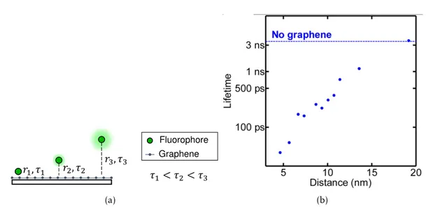
1.1 Fluorescence lifetime dependence on distance to graphene. (a) Shorter dis-tances yield stronger RET and therefore shorter lifetimes. (b) Experimental evidence of the interaction by Gaudreau et al [25]. . . 3 1.2 DNA-beacon biosensor experiment schematic. A graphene surface is

func-tionalized with fluorescently labeled DNA-beacons (probe DNA) and the flu-orescent lifetime is characterized before and after the addition of complemen-tary (target) DNA. The hybridization of probe and target DNA produces a nanoscale increase in the fluorophore distance to graphene and therefore an increase in the fluorescence lifetime which, from the biosensing point of view is indicative of the presence of target DNA. . . 4

2.1 Fluorescence sequence. After radiation absorption, the molecule undergoes non-radiative decays to reach the vibrational ground-state. In the case of fluo-rescence, a radiative decay brings the molecule back to the electronic ground state. Figure adapted from [39]. . . 6 2.2 Two level energy scheme. Upon external excitation, the molecule is excited

from the ground states0to an excited states1with an absorption rateΓabsand return tos0 by means of a radiative or non-radiative decay, with the rate Γr andΓ

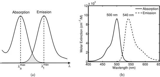
nr, respectively. . . 6 2.3 Absorption and emission spectra. Their shapes are characteristic of the

vi-brational structure of the upper and lower states, respectively. Absorption and emission often show a mirror-like image of each other and an overlap for certain wavelengths. (a) Derived model of the typical shapes of the spectra. Adapted from [40]. (b) Absorption an Emission spectra of fluorescein [41]. . 7 2.4 Fluorescence lifetime. (a) The influence of lifetime in the shape of the

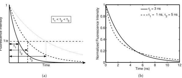
de-cay curve for a single-exponential dede-cay. (b) Single (full line) and double-exponential (dashed line) decays. Both curves have an average lifetime of 3 ns, however the dashed curve decreases sharply until 3 ns and smoothly afterwards. . . 9 2.5 Energy transfer mechanisms. (a) Non-radiative complex formation. (b)

(18)

L i s t o f F i g u r e s

2.6 Dynamic quenching scheme. A fluorophore is excited with an incident energy

hν and decays with the sum of radiative and non-radiative decay ratesΓ_r and Γ

nr, respectively. Upon interaction with a quencher molecule, an additional dynamic quenching decay rateΓ

dq appears. Figure adapted from [40] . . . . 10 2.7 Dependence of the transfer rate on the dimensionality of the acceptor

(Equa-tion 2.20). (a) Transfer between two point-dipoles: acceptor is 0D⇒n= 3. (b)

Transfer between a point-dipole and a two dimensional array of point-dipoles: the acceptor is 2D⇒n= 1 . . . 12

2.8 Time Correlated Single Photon Counting. Adapted from ref. [49]. (a) The measurement is performed at low fluorescent signal intensities so that the de-tection of more than one photon per pulse is highly unlikely. When photon is measured, its time arrival relative to the laser pulse is stored. (b) A histogram of photon time arrivals is built to produce a measure of the fluorescence decay curve. . . 15 2.9 Principle of a confocal microscope. A first pinhole reduces the illumination

on the sample and a second reduces the field of view coming from it. Thus, the measured signal comes from a very small volume of the sample. . . 16 2.10 Energy level diagram of Rayleigh and Raman scattering. The energy of the

emitted photon is shifted from that of the absorbed photon depending on the initial and final vibrational state. . . 17 2.11 Raman features of graphene. (a) Monolayer graphene Raman spectrum [60].

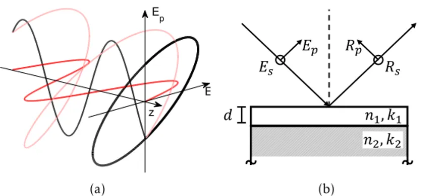
(b) Comparison of Raman spectra of graphite and graphene [61]. (c) Compar-ison of the Raman spectra for different layers in multi-layer graphene. . . 18 2.12 Ellipsometry. (a) Polarization ellipse of propagating light. (b) Reflection of an

incident beam on a film with thicknessd, refractive indexn1, and extinction coefficient_k₁.. . . 19 2.13 Self-complementarity of DNA beacon. When single-stranded, the molecule

assumes a folded configuration. DNA beacons are commercially available where at the endgroup a fluorescent dye is attached. . . 20 2.14 1-Pyrenebutyric acid N-hydroxysuccinimide ester (PBSE) linker molecule. (a)

Schematic of the molecule. (b) 3D representation of bonding with graphene. 21

(19)

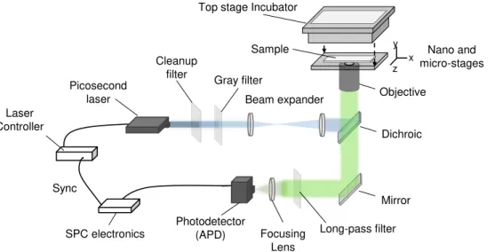
3.2 Scheme of the custom built FLIM setup used in this thesis. A picosecond laser is expanded and guided to an inverted microscope equipped with a high Numerical Aperture (NA) objective and an Avalanche Photodiode (APD) in confocal geometry. Suited filters guide the laser to the sample, while longer wavelength emission can pass the dichroic filter as well as the long pass fil-ter placed in front of the detector. The APD generates NIM pulses which are read out by fast Single Photon Counting (SPC) electronics allowing the collection of Time-Correlated Single Photon Counting (TCSPC) traces. The sample is scanned via nano- and micropositioning system, while temperature and humidity of the sample are controlled via a top stage incubator. . . 26 3.3 Graphene deposition and transfer process. (a) Chemical Vapor Deposition

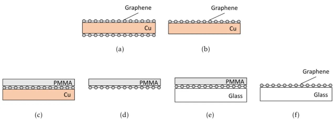
(CVD)-grown graphene on both sides of a Cu foil. (b) Graphene is plasma-ashed from one side. (c) A Poly(methyl methacrylate) (PMMA) thin film is spin-coated on the graphene. (d) Cu foil is dissolved using a FeCl3solution. (e) The sheet is transferred onto a microscope glass coverslip. (f) The PMMA film is dissolved in acetone and the transfer process is finished. . . 28 3.4 Surface functionalization procedure. (a) Graphene substrate. (b) Graphene

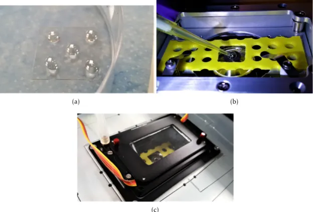
functionalization with 1-Pyrenebutyric Acid N-Hydroxysuccinimide Ester (PBSE) linker. (c) Drop-casting of biosensor-probe DNA. (d) Passivation of surface with ethanolamine to remove remnant PBSE. . . 31 3.5 Fluorescence lifetime-based DNA molecular beacon biosensor experiment.

(a) Five 10 µl samples drop-casted on a graphene surface on a microscope

glass coverslip. (b) Addition the target DNA solution during FLIM measure-ment session. (c) Temperature and humidity control chamber mounted on the nanopositioning stage of the of the FLIM setup to prevent sample evaporation. 33

4.1 Schematic of the calibration sample’s design. (a) SiO2spacer steps introduce well defined nanometer nanometer sized distances between a fluorescent dye (fluorescein) and graphene. (b) Schematic with the dimensions of the sample. 36 4.2 Graphene transfer results. (a) Graphene sheet deposited around a Cu foil. (b)

PMMA film deposited on top of graphene sheet. (c) Graphene on a PMMA film after the Cu foil dissolution in FeCl3. (a), (b) and (c) correspond to the steps shown in Figures 3.3(a), 3.3(c) and 3.3(d), respectively. . . 36 4.3 Dark-field optical microscopy image of graphene sample. The enhanced

(20)

4.4 Raman spectroscopy analysis of graphene sample. (a) Comparison between non-defect and defect graphene Raman spectra. For the red line, the relatively small intensity of the D peak and the rationI2D/IG≈2 indicate a small number of significant defects and the presence of monolayer graphene, respectively. (b) 300×300µm Raman map of graphene sample. The red and blue areas in

encode the spectral correlation with the spectra in (a). . . 38 4.5 Successive SiO2depositions to form discrete spacing between graphene and

fluorophores. A moving shutter partially blocks the SiO2deposition, allowing the steps to form. (a) Photograph of shutter implementation. (b) Optical interferometer measurement of SiO2 thickness profile. In this plot, the zero has been set at the top of a 100 nm thick SiO2layer on a Si wafer, which were deposited merely for enhanced interferometer accuracy purposes. . . 39 4.6 Ellipsometry results. The thickness of the Polyvinyl alcohol (PVA) layer has

been derived from the model used to fit the ellipsometry measurements. (a) Measurement results (full lines) and fitting models (dots). (b) Structure of the model used for fitting the results of (a). . . 40 4.7 Fluorescence intensity of alignment microsphere with 0.5 µm in diameter.

The shape and diameter of the image was used to estimate the lateral error of the custom-built semi-confocal FLIM setup. The lateral resolution is usually obtained by imaging microspheres with diameters below the diffraction limit (0.1µm for instance), however in this case this was not possible. (a)

Fluores-cence intensity image of the bead. (b) Intensity profile of the image at the location of maximum intensity. . . 42 4.8 Fluorescence intensity images of fluorescein deposited on graphene samples.

Dark blue areas correspond to graphene flakes and orange areas correspond to the glass surroundings. (a) Single measurement of 200×200µm2showing

small graphene flakes . (b) A 600×800µm2scan composed of twelve 200×

200µm2measurements appended together in a 3:4 matrix shows a much more

homogeneous graphene surface coverage than that of (a). . . 42 4.9 Fluorescence images of fluorescein deposited on a graphene flake. (a)

Fluo-rescence intensity image. (b) FluoFluo-rescence lifetime image. Both fluoFluo-rescence intensity and lifetime of the Fluorescein layer are reduced upon the presence of a graphene patch.. . . 43 4.10 Fluorescence lifetime distribution of the FLIM image from Figure 4.9(b). (a)

(21)

4.11 FLIM images of each spacer step of the nanofabricated calibration sample. The top-left insets on the images indicate the SiO2spacer thicknesses. As a conse-quence of the near-field RET interaction of fluorescein with the graphene, the fluorescence lifetime is highly dependent on the nanoscale distance, showing a remarkable reduction for shorter distances. . . 46 4.12 3Dwaterfallrepresentation of fluorescence lifetime distributions as function

of SiO2 thickness. The red dots at the top of the box indicate the modes of each distribution. These shall be the values used for the determination of an experimental fluorescence lifetime-distance calibration curve.. . . 46 4.13 Fluorescence lifetime-distance calibration curve. (a) Characteristic lifetimes

of each of the FLIM images of Figure 4.11 obtained by calculating the mode of their lifetime distributions (Figure 4.12). The fluorescence lifetime shows a clear dependence with the distance, however there seems to be a discontinuity for SiO2thicknesses between 7.9 nm and 10.2 nm. (b) Comparison between the results of (a) and the theoretical model derived in Section 2.1.4.2 (Equa-tion 2.24). The fluorescence lifetimes for SiO2thickness above or equal to 10.2 nm appear to be in better agreement with theory than those for SiO2thickness below 10.2 nm.. . . 47 4.14 Derived model of a thick fluorescent film, where multiple fluorophores within

the excitation volume of the laser are contributing to the fluorescence signal. Even ifd1= 0 nm, the average lifetime of the contribution of the three fluo-rophores is larger than zero. The non-zero thickness of the fluorescent film is therefore masking the shorter lifetime contribution. . . 48 4.15 Fluorescence lifetime-distance results calculated using Instrument Response

Function (IRF) deconvolution and reconvolution algorithms. (a) Comparison with the theoretical model presented in Section 2.1.4.2 (Equation 2.24). The IRF reconvolution results show a similar slope for SiO2thicknesses above 10.2 nm, but an overall larger error than the IRF deconvolution. (b) Derived semi-empirical model. The blue dashed line was obtained by ignoring the measure-ments below 10.2 nm and modifying the model presented in Section 2.1.4.2, using a free-space lifetimeτ0= 2.8nsand inserting an experimental coefficient in the dielectric functionAǫ, whereA= 1.92. . . 49

(22)

4.17 Conjugation of N-Hydroxysuccinimide (NHS)-Ester modification to amino-labeled oligonucleotide. The DNA sequence corresponds to the fluorophore(Atto-488)-labeled DNA molecule used in the biosensing experiments. . . 51 4.18 FLIM images of the DNA-beacon biosensor sample before and after reaction

with target DNA. (a) Initial state of the biosensor. Most of the area is covered with short fluorescence lifetimes which result from the strong RET between the atto-488 label fluorophores and the graphene. The longer lifetimes correspond to non-specifically bound beacons which resisted the surface passivation pro-cedure. (b) Final state of the biosensor. Large fraction of the image shows a remarkable increase in fluorescence lifetime relative to (a) where beacons hybridized with target DNA. Short lifetime areas a likely to correspond to empty glass without any graphene or beacons. . . 53 4.19 Derived molecular model of the DNA-beacon unfolding process. (a)

Ini-tial state of the biosensor. Biosensor-probe DNA molecules are attached to graphene but also to glass by non-specific binding. The fluorescence lifetime of the fluorophore labeled beacons attached to graphene is reduced by RET, but remains unchanged for those on the glass surface. (b) Final state of the biosensor. Biosensor-target DNA molecules hybridized with all beacons, but only those attached to graphene display an increase in their fluorescence life-time. . . 54 4.20 Fluorescence lifetime distribution before and after reaction with biosensor

target DNA. (a) Histograms of fluorescence lifetime at the initial (red) and final (black) states of the biosensor. Hybridization lead to the appearance of a distinct feature aroundτ∈[2.5;3.7] ns, corresponding to the lifetime of the

DNA beacons in the stretched configuration. (b) Difference between reduced fluorescence lifetime distribution images before and after hybridization. The reduced lifetime distribution images of Figures 4.18(a) and 4.18(b), were ob-tained analogously to the treatment in Section 4.1.2.2 and then subtracted. The resulting image highlights the areas in which there was a lifetime increase: thebiosensor active areas. . . 55 4.21 Identified areas of interest obtained by isolating areas from Figure 4.20(b)

(23)

4.22 Lifetime distribution of isolated areas of interest from Figure 4.21(a) to 4.21(c) and respective Gaussian fits. The derived molecular illustrations of Figure 4.19 were used as legends. From short to longer lifetimes, the Gaussian peaks cor-respond to: (blue) Active area before addition of target DNA @(t=0 mins)(τ_c= 0.40, Full Width at Half Maximum (FWHM)= 0.31) ns; (green) active area

after addition of target DNA @(t=125 mins)(τc= 1.72, FWHM= 0.35) ns; (red) Non-specific binding @(t=0 mins)(τ_c= 2.00, FWHM= 0.20) ns. In the derived lifetime to distance model the change from 0.4 to 1.7 ns is associated with an

≈10 nm translocation of the fluorescent labels (from round 9 nm to 19 nm)

away from the graphene surface. . . 56 4.23 Fluorophore distance to graphene. The distance was calculated by

apply-ing the semi-empirical model derived in Section 4.1.4 to the FLIM image of Figure 4.21(b) and subtracting the background level of 9.27 nm. (a) Spatial distribution of fluorophore distance to graphene. (b) Histogram of distance occurrences. The molecular length of the DNA sequence was estimated to be 8.4±2.3 nm . . . 57

4.24 3D representation of the biosensor before (a) and after (b) the addition of target DNA. A large fraction of the scanned area shows an increase of 8.4±2.3 nm

in the fluorophore distance to graphene after hybridization. Regions where non-specific binding occurred show distances tending to infinity (colored in white). . . 58 4.25 Time lapse FLIM images of the graphene-based DNA-Beacon biosensor after

the addition of target DNA. A total of 52 images were acquired, with a collec-tion time of 4 minutes and 45 seconds per image, showing the hybridizacollec-tion process from 10 to 252 minutes. The time points are given at the top-left corner of each image. . . 59 4.26 Time-lapse fluorescence lifetime distributions of the DNA molecularr beacon

biosensor during DNA hybridization. (a) Histograms of 52 FLIM measure-ments. The modal value of the distributions shifts continuously over time (Mo(t = 10 min)≈0.54 ns→Mo(t= 10 min)≈1.30ns) indicating a

(24)

4.27 (a) Time-dependent abundance of the identified characteristic fluorescence lifetimes per FLIM image. The most abundant component at the beginning of the reaction (dark blue - shorter lifetimes) completely vanished after about 150 minutes. An intermediate state (cyan - intermediate lifetimes) increased to a maximum and decreased afterwards, showing a lifespan of about 85 min-utes. The final states (green and orange - longer lifetimes) show a prominent increase at the moment the intermediate state started to decrease. The longest lifetime component (red) shows free-space lifetime of the fluorophore (≈2 ns).

(b) Linear anti-correlation between the lifetime distribution at a given time point and initial state. From an applied perspective, the shape of this curve qualitatively indicates the kinetics of the reaction. It shows a sharp increase for reaction times between 85 and 160 minutes and a saturation point at 185 minutes (room temperature 19◦_Celsius). _{. . . .} ₆₁

4.28 Derived molecular model of the DNA unfolding process during hybridization with the target DNA. The temporal analysis of the kinetics of hybridization revealed the existence of intermediate states, where the biosensor probe and target DNA are only partially bonded. . . 62 4.29 Fluorescence lifetime determination using exponential curve-fits. (a)

Single-exponential fit. The resulting curve does not properly fit the experimental points. (b) Double-exponential fit. The resulting curve fits the experimental points nearly perfectly (c) triple-exponential fit. The third exponential is not necessary to fit the experimental points. . . 64 4.30 TCSPC measurement of the IRF. The instrument’s response to an infinitely

short light pulse as a consequence of the transit-time spread of the photo-electrons through the detector. The IRF can be taken as the signature of the particular custom-built setup used in the measurements and its effects should be compensated in the determination of the fluorescence lifetime. . . 64 4.31 Experimental decay curves (dots) and multi-exponential fits (dashed lines) for

three different fluorescence lifetimes. (a) Using a modeled IRF reconvolution. (b) Using a measured IRF deconvolution. Fluorescence lifetimes calculated using IRF deconvolution are consistently lower than those for which IRF re-convolution was used. . . 65 4.32 Intensity threshold lifetime determination method. (a) Measurement of the

IRF and two example curves. (b) The lifetime is given by difference between the times at which the integrals of a given measurement and the IRF reach the intensity threshold 1−1/e. The matrix calculations can be performed for

(25)

4.33 Comparison between different lifetime determination models and integration times (tinteg). (a) IRF deconvolution algorithm (tinteg= 138.03 s). (b) IRF recon-volution algorithm (tinteg= 37.27 s). (c) Intensity threshold algorithm(tinteg= 1.97 s). (d) Fluorescence lifetime distributions of the images in (a), (b) and (c). The intensity threshold method spreads over a fluorescence lifetime span that is intermediate to the other two algorithms, but took far less time to inte-grate. In the FLIM images, the IRF deconvolution shows perhaps the clearest structural contrast. . . 67 4.34 Comparison of distance-dependent fluorescence lifetime calibration curves,

calculated with the three diff_{erent models. The results are compared with} the theoretical model from Gaudreau et al [25] and the semi-empirical model derived in Section 4.1.4. . . 68 4.35 FLIM analysis interface of toolbox developed for MATLAB. The user can select

a folder with multiple data files and the file to be open on the left pane. (a) Data visualization tab. The fluorescence intensity image and singular TCSPC measurements can be visualized. (b) Fluorescence lifetime analysis tab. The FLIM image, fluorescence lifetime distribution and reduced fluorescence life-time image can be calculated and are displayed together in the same window. 70

(26)

(27)

L i s t o f Ta b l e s

3.1 Deposition times for depositing a 100 nm SiO2layer on an auxiliary Si wafer and seven 3 nm SiO2 layers on both auxiliary and graphene sample. The deposition times were derived by considering a deposition rate of 0.789 nm.s−1

for the 100 nm and 0.801 nm.s−1_{the 3 nm.}_{. . . .} ₂₉

3.2 Parameters for the double stepped Spin-coating of fluorescein-doped layer. . 30 3.3 Sequence of nucleobases of the DNA molecules used for the testing of a hairpin

molecular DNA-Beacon biosensor. . . 30

4.1 Mean and standard deviation of the thickness (h) of each step in the

interfer-ometer results of Figure 4.5(b). . . 39 4.2 Derived fluorescence lifetime-diff_{erence thresholds and respective}

designa-tions, for the identification of structures in Figure 4.20(b). In areas outside of graphene were separated in void areas, where no DNA beacons attached andnon-specific binding areaswhere DNA beacons attached to glass instead of graphene. In both cases the fluorescence lifetime remained nearly constant (δτ≈0 ns) however their initial lifetimesτ₀are different. . . 54

4.3 Calculated fluorophore-graphene substrate distance, based on the semi-empirical model from Equation 4.8. The errors have been calculated using the standard deviations of the Gaussian peaks in Figure 4.22. . . 57 4.4 Conversion of the identified characteristic fluorescence lifetime components

of the hybridization reaction to nanoscale distances. The conversion of fluores-cence lifetime to distance was performed analogously to the analysis presented in Section 4.2.3. The free-space lifetime was considered to beτ0= 2 ns, and therefore r(τ =τ0)→ ∞, which stands for fluorophores in solution located

outside the range of RET to the graphene. . . 60

A.1 The "flim" structure. List of all the fields and sub-fields where data is stored in the flim structure. . . 85 A.2 Structure of the Nanophotonics toolbox. The numbers in brackets indicate the

(28)

(29)

A c r o n y m s

APD Avalanche Photodiode.

CPS Chance, Prock and Silbey.

CVD Chemical Vapor Deposition.

DMF Dimethylformamide.

DNA Deoxyribonucleic Acid.

FLIC Fluorescence Interference Contrast.

FLIM Fluorescence Lifetime Image Microscopy.

FRET Förster Resonance Energy Transfer.

FWHM Full Width at Half Maximum.

INL International Iberian Nanotechnology Laboratory.

IPA Isopropyl Alcohol.

IRF Instrument Response Function.

NA Numerical Aperture.

NHS N-Hydroxysuccinimide.

PBSE 1-Pyrenebutyric Acid N-Hydroxysuccinimide Ester.

PECVD Plasma-Enhanced Chemical Vapor Deposition.

PMMA Poly(methyl methacrylate).

PVA Polyvinyl alcohol.

RET Resonance Energy Transfer.

(30)

AC R O N Y M S

SPC Single Photon Counting.

TCSPC Time-Correlated Single Photon Counting.

(31)

C

h

a

p

t

e

r

1

I n t r o d u c t i o n

1.1 Motivation and importance of the work

Biosensing has been gaining more and more relevance as a technique in applications rang-ing from medical purposes to food-quality tracrang-ing, includrang-ing the prevention of outbreaks of food-borne illnesses and in the combat against attempts of fraudulent malpractice in billion euro businesses. Particularly, the use ofDeoxyribonucleic Acid (DNA)-based de-tection systems revolutionized biosensing for introducing reliable methods of biological fingerprinting. However, most of the established techniques forDNAbiosensing merely output "on-off" electrochemical signals at the presence of specific molecules, which makes

them poorly descriptive of the system and its interactions. A new generation of DNA biosensors however, rises with the application of graphene a sensing platform.

In recent years, graphene has been shown to hold extraordinary optical, electronic and mechanical properties, revealing a fascinating versatility for endless applications. Among its qualities, its strong non-radiative electromagnetic coupling to light-emitting molecules, has recently left its mark in the world of nanoscale distance sensing, for enabling a reversible distance-dependent fluorescence lifetime reduction when at the nanoscale vicinity of fluorescent dyes.

This work brings together the virtues of the two techniques by using the lateral reso-lution ofFluorescence Lifetime Image Microscopy (FLIM)for a spatial characterization of the biosensing platform and the nanoscale axial resolution provided by the interaction with graphene for the implementation of aDNAbiosensor through the measurement of molecule-sized distances.

(32)

C H A P T E R 1 . I N T R O D U C T I O N

1.2 State of the Art

At the beginning of this century, most high-resolution fluorescence-based microscopy techniques could only provide resolution in the lateral directions [1]. Indeed, only Total-Internal Reflection Fluorescence (TIRF)[2] andFluorescence Interference Contrast (FLIC) [3] stood out for their resolution in the axial direction. However, these techniques (and many others) relied on the measurement of fluorescence intensity, which is highly vulner-able to intrinsic spatial and temporal fluctuations, mainly due to heterogeneous labeling and photobleaching. Alternatively,FLIM[4,5] stood out for its independence of concen-tration and photobleaching [6] and great success in the labeling and study of dynamic live cellular structures [7,8,9], yet again it was only able to provide lateral resolution.

On a complementary level, fluorescent molecules have been known to interact with other molecules and theoretically studied since the 1940’s [10,11]1. In 1948, Theodor Förster published in German his worldwide highly cited paper describing the principles of intermolecular energy transfer [11]. It described the resonant energy transfer between the oscillating dipoles of a fluorescence emitter and an energy acceptor in its surround-ings, leading to what eventually became universally known byFörster Resonance Energy Transfer (FRET). In the 1960’s the fluorescence lifetime of fluorophores near metal sur-faces was studied [14], leading to the famous Chance, Prock and Silbey (CPS) model [15] and many other publications regarding the interaction of fluorescent molecules near metal interfaces, by the 1980’s [16,17]. More recently, the distance dependence of fluores-cence quenching and lifetime reduction by metal nanostructures has been studied, such as gold nanoparticles [18, 19, 20]. In the last decade, axially-resolved nanometer and sub-nanometer accuracy optical rulers have been studied from interactions with metallic thin films [21,22,23], transparent conductive oxides [24] and ultimately for graphene [25,26,27,28]. In particular, Gaudreau et al [25] experimentally quantified the distance dependence of fluorescence lifetime with the distance to graphene (see Figure1.1) due to FRET. Their results are in good agreement with previously derived theoretical models [29, 30]. These works together opened new routes for innovation in biosensing technologies.

Simultaneously to the progresses in the understanding of interactions of fluorescent dyes with 2D layers and materials like graphene, in the field of biotechnologies, huge advances inDNAbiochemistry were made. Last-decade research has provided a remark-able broadening of nanoscale biological understating and bio-applications, namely in the DNAbiochemistry and biosensing areas [31,32], which have great impact in health and food-quality tracing [33, 34]. SeveralDNA hybridization-based biosensors have been implemented [35] such as the hairpinDNAmolecular beacon [36], which relies on the configuration change of aDNA-beacon (probeDNA) upon hybridization with a comple-mentary targetDNA[37,38]

Particularly, a number ofDNA-based biosensing devices has been developed with

(33)

1 . 3 . O B J E C T I V E S A N D G OA L S

𝑟2, 𝜏2 𝑟3, 𝜏3

𝑟1, 𝜏1

Graphene Fluorophore

𝜏1< 𝜏2< 𝜏3

(a) (b)

Figure 1.1: Fluorescence lifetime dependence on distance to graphene. (a) Shorter dis-tances yield strongerRETand therefore shorter lifetimes. (b) Experimental evidence of the interaction by Gaudreau et al [25].

applications ranging from medical purposes to food-quality tracing techniques [33]. In the latter scope, which encompasses the prevention of outbreaks of food-borne illnesses [33] and the combat against attempts of fraudulent malpractice in billion euro businesses [34].

1.3 Objectives and Goals

The main goals of this master thesis are: a) the study of the dependence of the fluores-cence lifetime of fluorophores at nanoscale distances to graphene for the development of a nanoscale distance sensing technique, using recently described graphene near-field effects; and b) the validation of this technique’s applicability in biosensing, by the

devel-opment of a fluorescence lifetime-basedDNAmolecular beacon biosensor (Figure1.2). For this purposes, it is required the design and nanofabrication of a calibration sample that allows obtaining nanoscale distance information from fluorescence lifetime mea-surements and the surface functionalization of graphene with biosensor-probe DNA molecules, such that time-lapseFLIMmeasurements of the hybridization process upon the addition or targetDNAmolecules can be used as a biosensing technique.

(34)

C H A P T E R 1 . I N T R O D U C T I O N

Perfect match solution

DNA-Beacons bound to graphene

Hybridized (stretched) DNA-Beacons

(35)

C

h

a

p

t

e

r

2

T h e o r e t i c a l Ba c k g r o u n d a n d P r i n c i p l e s

2.1 Physical Principles

2.1.1 Fluorescence

Fluorescence is the emission of light by a molecule that has been excited by some form of electromagnetic radiation. In particular, it is the consequence of a radiative electronic transition from an excited state to a lower energy level. Following the Franck–Condon principle, when a molecule is optically excited it will most likely be excited onto a higher-energy vibrational level within the excited electronic level (see Figure2.1). At that point, it will release part of it energy by non-radiative decay to reach the vibrational ground-state and finally return to the electronic ground ground-state by means of either a nonradiative or a radiative decay (fluorescence emission). [39].

The measured fluorescence intensityIf can be written as a function of overall detec-tion efficiency_kand fluorescence quantum yield_φ_f as

If =kφfI0(1−10−αcl) (2.1)

wherekis the detection effi_ciency,_φ

f is the quantum yield,α is the molar absorption coefficient,_cis the molar concentration of the fluorescent dye and_lis the light path length

within the sample. The quantum yield is defined as

φf ≡

Number of photons emitted Number of photons absorbed =

Intensity of light emitted

Intensity of light absorbed (2.2) Considering a simple two-level model as the one depicted in Figure2.2, the number of molecules in the excited state s1 varies with the difference between the number of

(36)

C H A P T E R 2 . T H E O R E T I CA L BAC KG R O U N D A N D P R I N C I P L E S Absorption Emission (Fluorescence) P ot en ti al E ner gy Internuclear separation Non-radiative decays

Figure 2.1: Fluorescence sequence. After radiation absorption, the molecule undergoes non-radiative decays to reach the vibrational ground-state. In the case of fluorescence, a radiative decay brings the molecule back to the electronic ground state. Figure adapted from [39].

E

Γ

𝑎𝑏𝑠

Γ

𝑛𝑟

Γ

𝑟

𝑠

1

𝑠

0

Figure 2.2: Two level energy scheme. Upon external excitation, the molecule is excited from the ground states0to an excited states1with an absorption rateΓabs and return to

s0by means of a radiative or non-radiative decay, with the rateΓr andΓnr, respectively.

dn1

dt =Γabsn1−(Γr+Γnr)n1 (2.3)

whereΓ

abs,ΓrandΓnr are the absorption rate and radiative and non-radiative decay rates, respectively.

Considering that an equilibrium state is achieved (steady-state), where the number of molecules transiting into the excited states1matches the number of molecules transiting

out of it, the rate dn1/dt becomes zero and Equation2.3can be written as

Γ

absn1= (Γr+Γnr)n1 (2.4)

In such case, intensity of light absorbedIabs=Γabsn1and the intensity of light emitted Iemi =Γrn1and the two intensities can be replaced in Equation2.2to form

φf =

Γ r Γ_r+Γ_nr

n1

n1 =

Γ r

Γ_r+Γ_nr (2.5)

(37)

2 . 1 . P H YS I CA L P R I N C I P L E S

2.1.1.1 Absorption and emission spectra

Both the absorption and emission of radiation are energy-dependent and therefore wave-length dependent (E=hc/λ). As a consequence, the quantum yield, can be expressed as

the sum of all steady-state fluorescence intensity per absorbed photonsF(λf) as function of the wavelength of the emitted photonsλf [40] by

φf =

Z ∞

0 F(λf)λfdλf (2.6)

whereF(λf) is the molecule’s fluorescence emission spectrum and the shape of its plot is characteristic of the vibrational structure of the lower electronic state. For the absorp-tion, the productα(λa)clrepresents the wavelength-dependent absorption spectrum and the shape of its plot is characteristic of the vibrational structure of the excited upper state. Due to the diff_{erent excitation-relaxation possible transition combinations, the}

emission and absorption spectra often show a mirror image of each other, with an over-lap (Figure 2.3(a)). Figure2.3(b)shows the measured emission spectra for fluorescein [41]. Wavelengths corresponding to the absorption-emission overlap may result in auto-excitation and therefore to theinner filter effect, which can induce significant changes in

the emission spectrum and fluorescence lifetime.

Additionally, the absorption of light occurs most efficiently along the direction of its

absorption moment [40]. For an unpolarized light source, only part of the radiation is absorbed and therefore the coupling between excitation light beam and average transition moment of the fluorophores must be taken into consideration in the excitation efficiency.

λ_amax _λ f max Absorption Emission

λ

(a)

4000 450 500 550 600 650

2 4 6 8 10

12x 10

4

Wavlength (nm)

Molar Extinction (cm

−1

/M)

Absorption Emission 500 nm 540 nm

(b)

(38)

C H A P T E R 2 . T H E O R E T I CA L BAC KG R O U N D A N D P R I N C I P L E S

2.1.2 Fluorescence Lifetime

The fluorescence lifetime is the average time that an excited fluorescent molecule takes to decay from an excited states1back to the ground states0. Considering a pulsed excitation

source, at the moment when the excitation source is switched offthe absorption rateΓ abs becomes zero, and Equation2.3becomes [42]

dn1

dt =−(Γr+Γnr)n1 (2.7)

whose solution is:

n1(t) =n1(0)e−(Γr+Γnr)t=n1(0)e

−t

τf _(2.8)

whereτf is the fluorescence lifetime

τ_f =_Γ 1

r+Γnr

(2.9)

Interestingly, the quantum yield from Equation2.5can be related to the fluorescence lifetime as

φf =τfΓr (2.10)

which replaced in Equation2.1expresses the fluorescence intensity dependence on the fluorescence lifetime.

According to Equation2.8, the fluorescence intensity over time assumes the form of an exponential decay whose fluorescence lifetime τf is an intrinsic characteristic of the fluorophore (see Figure 2.4(a)). In practice however, apart from single-molecule measurement conditions, a measured fluorescence decay is most likely the result of the contribution from several fluorophores in the sample, which may have different lifetimes.

In such cases, the measurement will take the form of multi-exponential decay

I(t) =

n X

i

(Ii0e−t/τi) (2.11)

where the relative intensityI_i₀/Pn

iIi0of each lifetime is proportional to their

concentra-tion and quantum yield1_{. In this case, a weighted average lifetime is commonly defined} by

τf =

Pn i(Ii0τi) Pn

i Ii0 (2.12)

Figure2.4(b)shows the diff_{erence in shape between a single (full line) and double}

(dashed line) exponential curve. In the double exponential curveI10=I20= 1/2, both

1_{A first order Taylor approximation of Equation}_2.1_yields_I

f ≈klog(10)φ_fI₀αclfor low concentrations

(39)

2 . 1 . P H YS I CA L P R I N C I P L E S Time Fluorescence Intensity τ₃ τ₂ 1 1/e

τ₁ < τ₂ < τ₃

τ₁

(a)

0 2 4 6 8 10 12

0 0.2 0.4 0.6 0.8 1 Time (ns)

Normalized Fluorescence Intensity

τ_f = 3 ns

τ₁ = 1 ns, τ₂ = 5 ns

(b)

Figure 2.4: Fluorescence lifetime. (a) The influence of lifetime in the shape of the decay curve for a single-exponential decay. (b) Single (full line) and double-exponential (dashed line) decays. Both curves have an average lifetime of 3 ns, however the dashed curve decreases sharply until 3 ns and smoothly afterwards.

curves have an average lifetime of 3 ns, however the two curves carry very distinct infor-mation. Diff_{erent lifetimes may surge due to di}ff_{erent fluorescent species or due to the}

occurence of lifetime reduction mechanisms.

2.1.3 Fluorescence Quenching and Lifetime Reduction

The fluorescence lifetime, quantum yield and emission spectrum can be aff_{ected by the}

surrounding medium. In particular, the fluorescence intensity can be quenched by means of physical or chemical interactions withquenchers[40,42].

Four diff_{erent mechanisms can be defined as [43]: Non-radiative complex}

forma-tion, where the energy is used in the chemical formation of a non-fluorescent product (Figure 2.5(a)); Collision quenching, where the energy is lost to another molecule by physically colliding with it (Figure2.5(b)); Re-absorption, where a photon with energy within the absorption-emission overlap is emitted by a fluorophore and absorbed by an-other (Figure2.5(c)); andResonance Energy Transfer (RET), where there is a radiationless electromagnetic energy transfer from a fluorophore to a quencher by means of a resonant interaction (Figure2.5(d)).

(40)

C H A P T E R 2 . T H E O R E T I CA L BAC KG R O U N D A N D P R I N C I P L E S ( ) * * + (a) * _* (b) * + * ℎ𝜈 (c) * + * + (d)

Figure 2.5: Energy transfer mechanisms. (a) Non-radiative complex formation. (b) Colli-sion quenching. (c) Re-absorption. (d) Resonant Energy Transfer

ℎ𝜈

Γ𝑟+ Γ𝑛𝑟

… + + * Γ𝑞 Fluorophore Quencher molecule * Excited state

Figure 2.6: Dynamic quenching scheme. A fluorophore is excited with an incident energy

hν and decays with the sum of radiative and non-radiative decay ratesΓ

randΓnr, respec-tively. Upon interaction with a quencher molecule, an additional dynamic quenching decay rateΓ

dqappears. Figure adapted from [40]

2.1.3.1 Dynamic quenching and Stern-Volmer kinetics

The Stern-Volmer kinetics are usually applied for interactions between fluorophores and single molecules (0D), however, its elucidating equations can be generalized for acceptors with any dimensionality. The schematic image of Figure2.6 shows a simplistic model of the dynamic quenching. The fluorophores are excited with a photon energy hν and decay back to the ground state with a total rateΓ

r+Γnr, as they would in free-solution. At the presence of quencher moleculesQ, they transfer part of their energy toQat the

dynamic quenching rateΓ

q. Therefore, the number of fluorophores at the excited staten1 as function of time can be written as:

n1(t) =n1(0)e−(Γr+Γnr+Γq)t=e−t/τ (2.13)

where the lifetimeτ can be expressed as

τ= 1

Γ_r+Γ_nr+Γ_q (2.14)

According to Equation2.10, the quantum yield comes asφ=τΓ

r and therefore

φ= Γr

Γ_r+Γ_nr+Γ_q (2.15)

(41)

2.1.4 Resonant Energy Transfer

A great work has been done by Theodore Förster on this topic to develop a theoretical model of what is commonly known by the Förster Resonance Energy Transfer (FRET). Its formalism describes the interaction between two classical point-dipoles (donor and acceptor molecules) and quantifies the decay rate of the donor as function of the distance to the acceptor; its detailed deduction can be found in ref. [43].

Section2.1.4.1presents the main equations of this model and Section2.1.4.2presents an intuitive adaptation for the case ofRETto a graphene surface.

2.1.4.1 Förster Resonant Energy Transfer

According to Equation2.14, the decay rateΓ= 1_/τcan be written as

Γ=Γ₀+Γ

q (2.16)

whereΓ₀=Γ

r+Γnr is the unquenched total decay rate.

In Förster’s model the rate of energyWAbeing transferred to the acceptor is evaluated by solving the motion equation for a forced Harmonic oscillator. The quenching rateΓ

qis then calculated through

dWA

dt =ΓqWD (2.17)

whereWD is the energy being irradiated by the donor. The quenching rate results in

Γ_q= 1

τ₀

R0

r_AD

!6

(2.18)

whereτ0= 1/Γ0is the free-space lifetime of the donor,R0is the Förster distance andrAD is the distance between the donor and the acceptor. ReplacingΓ

q in Equation2.16, the total decay rate then becomes

Γ

Γ₀ = 1 +

R₀

rAD

!6

(2.19)

The Förster distance R0 corresponds to the distance at which the transfer rate ΓT matches the rate of decayΓ

r+Γnr. In other words, the probability of an excited molecule do decay to its ground state by fluorescence or any other non-radiative process is equal to the probability of transferring its energy to an acceptor at distanceR0. The dependence of

(42)

2.1.4.2 Resonant Energy Transfer to Graphene

The resonant energy transfer to a graphene is described by modeling the graphene surface as two-dimensional array of acceptor dipoles (Figure2.7). As a result, Equations2.18and 2.19are changed by the dimensionality of the acceptor [26]naccording to

Γ q=

1

τ0

R0(n)

r

!3+n

(2.20)

Γ

Γ₀ = 1 +

R0(n)

r

!3+n

(2.21)

whereR0(n) is the dimension-dependent Förster distance. To a 3D, 2D, 1D or 0D acceptor

corresponds ann= 0, 1, 2 or 3, respectively. Therefore, to the case of graphenen= 1 and the decay rate assumes a distance dependence of the formr−4_[46].

Gaudreau et al quantified the Förster distanceR0G for the case of graphene [25]

R0G=

9κ2αλ4

256π3(ǫ+ 1)2 (2.22)

which replaced in Equation2.21results in

Γ

Γ₀ = 1 +

9κ2α

256π3(ǫ+ 1)2 λ

r

!4

(2.23)

whereκ2is dipole orientation coefficient,_αis the fine structure constant (_α≈1/137 [47]), λ is the donor emission wavelength andǫ is the dielectric constant of the surrounding medium. A first approximation of the dipole orientation factor (0< κ2<4) yieldsκ2= 2/3

for an isotropic distribution [48].

Γ𝑇∝ 𝑟−6

(a)

Γ𝑇 ∝ 𝑟−4

(b)

Figure 2.7: Dependence of the transfer rate on the dimensionality of the acceptor (Equa-tion2.20). (a) Transfer between two point-dipoles: acceptor is 0D⇒n= 3. (b) Transfer

between a point-dipole and a two dimensional array of point-dipoles: the acceptor is 2D

(43)

In practice, it is customary to calculate fluorescence lifetimes, rather than decay rates. Equation2.23can be easily converted to lifetime by calculating its inverse form (τ/τ0=

(Γ_/Γ₀)−1_).

τ

τ0 =

1 1 +R0G/r4

(44)

2.2 Optical Technologies

This section presents a brief introduction to some of the optical techniques used in this work, whose results are discussed in chapter 4. It includes the concepts of Time-Correlated Single Photon Counting (TCSPC)for the measurement of time-resolved flu-orescent decays; confocal microscopy and how it can be used in Fluorescence Lifetime Imaging Microscopy (FLIM) and Raman spectroscopy - the Raman spectrum of graphene is also mentioned; and ellipsometry.

2.2.1 Time-Correlated Single Photon Counting

Time-Correlated Single Photon Counting (TCSPC)is the measurement of the arrival times from single photons emitted from a fluorescent dye upon repetitive excitation with short laser pulses [49]. Within the scope of time-resolved spectroscopy, the main challenge is the measurement of emission times which may last from hundreds of picoseconds to a few tens of nanoseconds, with intensities that may be as low as that of a single-fluorescent molecule regime.

Alternatively to photo-diodes and a fast oscilloscopes, which may at first glance seem like a reasonable approach, TCSPC systems overcome such difficulties by the repetitive

and precisely timed registration of single photons. Using the excitation pulse as time reference, a histogram of single photon’s arrivals is recorded in order to reproduce the time-resolved intensity profile of a fluorescence decay.

A key factor in this technique is to guarantee that indeed only single photons are counted (and not the summed eff_{ect of the arrival of multiple photons). This requirement}

can (and must) be met by the sufficient low light intensity that reaching the detector, such

that the probability of a detecting a photon arrival between two laser pulses becomes virtually zero. In other words, the detection of more than one photon per pulse is forced to be highly unlikely (Figure2.8(a)).

(45)

2 . 2 . O P T I CA L T E C H N O LO G I E S

Excitation Pulse

Photon Arrival

Δ𝑡1 Δ𝑡2

(a)

Arrival Time

Photon Counts

(b)

Figure 2.8: Time Correlated Single Photon Counting. Adapted from ref. [49]. (a) The measurement is performed at low fluorescent signal intensities so that the detection of more than one photon per pulse is highly unlikely. When photon is measured, its time arrival relative to the laser pulse is stored. (b) A histogram of photon time arrivals is built to produce a measure of the fluorescence decay curve.

2.2.2 Confocal Microscopy

Confocal microscopy is a sample- or laser-scanning microscopy technique, which uses light collimation to increase the spatial resolution. Figure2.9shows a schematic of the principle. The field of illumination projected onto the sample is reduced by placing a first pinhole in the microscope axis and focusing the light beam with a lens. Then, the field of view is limited further by placing a second pinhole in the image plane, confocally to the illumination spot in the sample and to the first pinhole [50]. The measured signal is therefore originating from a very small volume of the sample, at a fixed working distance to the objective.

(46)

Light Source Dichroic

Sample

Microscope Objective

Pinhole

Detector

Figure 2.9: Principle of a confocal microscope. A first pinhole reduces the illumination on the sample and a second reduces the field of view coming from it. Thus, the measured signal comes from a very small volume of the sample.

2.2.3 Fluorescence Lifetime Imaging Microscopy (FLIM)

Fluorescence Lifetime Image Microscopy (FLIM)is the spatial mapping of the fluores-cence lifetime distribution of a sample [4]. TypicallyTCSPCis combined with confocal microscopy in FLIM setups [51]. The main advantages ofFLIM over its fluorescence intensity-based alternatives are due its independence of intensity variations (namely due to photobleaching [6]), fluorophore concentration and excitation light-path, which can be difficult to control in biological systems [5].

TCSPCsystems require much shorter integration times compared with their analogic electronics, such as time-gated detection [52].

The spatial resolution of a confocal microscope is diffraction-limited, according to

Abbe’s diffraction limit:_d =_λ/(2_nsin_θ) and therefore approximately half the excitation

wavelength (typically between about 200-350 nm for visible wavelengths.

FLIMis widely used in cell biology studies [4,7, 8,9], as it can be used to monitor biochemical processes such as protein interactions [53], measurement of intracellular pH [54] and temperature [55].

2.2.4 Raman Spectroscopy

Raman spectroscopy is typically used for the observation of vibrational and rotational states in a molecule, by means of inelastic (Raman) scattering of photons [56].

(47)

Incident photon (E = ℎ𝜈1) Emitted photon (E = ℎ𝜈₂) Vibrational Ground state Vibrational Excited State Virtual Energy Level

ℎ𝜈1= ℎ𝜈2 Δ 𝜈 = 0

ℎ𝜈1> ℎ𝜈2 Δ 𝜈 > 0

ℎ𝜈1< ℎ𝜈2 Δ 𝜈 < 0

Rayleigh Stokes Anti-Stokes

Figure 2.10: Energy level diagram of Rayleigh and Raman scattering. The energy of the emitted photon is shifted from that of the absorbed photon depending on the initial and final vibrational state.

an induced dipole moment in the molecule (virtual energy level), whose emitted light contains the observed Raman scattering [58,59].

The scattering of light can occur in three different ways usually known by Rayleigh,

Stokes and anti-Stokes scattering. The Rayleigh scattering corresponds to the fraction of light with the same frequency as the incident light, whereas in the Stokes and anti-Stokes scattering there is a shift in the emitted photon energy which can either be lost (Stokes) or gained (anti-Stokes) in the molecule.

If the incident and emitted photons have energiesE1=hν1andE2=hν2, respectively,

where ν = c/λ is the light frequency and λ is the wavelength, then the diff_{erence in}

wavenumber of the two photons is given by

∆_νˆ=1

c(ν1−nu2) =

1 λ1 − 1 λ2 ! (2.25)

This is known by the Raman shift and is usually measured in cm−1_{(see Figure}_2.10). In terms of energy levels, when a molecule is excited from the vibrational ground state to the an excited virtual energy level, it can return to either the vibrational ground state (Rayleigh scattering) or to an excited vibrational level (Stokes scattering). Alternatively, if the molecule is already at an excited vibrational state before being excited into a virtual energy level, then it may de-excite onto an energy level with lower energy than that of its initial state (anti-Stokes scattering). Hence, the Raman shift∆_νˆcarries information of the intrinsic vibrational energy structure of the molecule, which can be used as a fingerprint for molecule identification purposes.

2.2.4.1 Raman Spectrum of Graphene

Monolayer graphene is most commonly identified by considering three main features in its Raman spectrum commonly denoted by the D, G and 2D peaks (∆_νˆ

D ≈1360 cm−1, ∆_νˆ

(48)

(a) (b) (c)

Figure 2.11: Raman features of graphene. (a) Monolayer graphene Raman spectrum [60]. (b) Comparison of Raman spectra of graphite and graphene [61]. (c) Comparison of the Raman spectra for different layers in multi-layer graphene.

order degree of carbon atoms and the 2D peak is the result of a second-order process involving two phonons with opposite momentum [60,61] - see Figure2.11(a).

In simpler terms, a low intensity of the D peak can be interpreted as an indicator of the graphene quality, and the G and 2D peaks can be regarded as the fingerprint peaks of Graphene, where an intensity ratio of peaks 2D over G larger than 2 is a typical feature of monolayer graphene. In that sense, Figure2.11(b)shows a comparison between the Raman spectra of graphite and monolayer graphene, highlighting the difference in the

intensity ratio of peaks 2D over G for the two cases and the broadening of the 2D peak from a single Lorentzian for the case of graphene to a double Lorentzian peak shape for the case of graphite. Indeed, as is shown in Figure2.11(c)this double-peaked shape of the 2D component intensifies progressively with the number of layers.

Raman spectroscopy measurements can also be performed in a confocal setup, for spatial mapping of the Raman features of a sample.

2.2.5 Ellipsometry

The geometric orientation of the electric field of a propagating monochromatic light beam can be expressed in terms of two transverse componentsEp andEs. Plotting the electric filed vector E = Ep+Es over a full oscillation cycle leads to an elliptical shape - the polarization ellipse (Figure2.12(a)).

The name ellipsometry arises from the measurement of the polarization ellipse. Briefly, ellipsometry is a measurement of the change in the polarization of a beam of light upon reflection on a surface - usually coated with a thin film (Figure2.12(b)). In practice, the measurements are compared with models such that optical parameters like the thickness

d, refractive indexnor extinction coeffi_cient_k_{of thin film can be extracted. In summary,}

if the incident and reflective fields are written as function of their phases (neglecting z

(49)

E

p

E

s

z

(a)

𝐸𝑝 𝐸𝑠

𝑅𝑝 𝑅𝑠

𝑑 𝑛1, 𝑘1

𝑛2, 𝑘2

~

(b)

Figure 2.12: Ellipsometry. (a) Polarization ellipse of propagating light. (b) Reflection of an incident beam on a film with thicknessd, refractive indexn1, and extinction coefficient

k1.

Em=E0meiαm (2.26)

Rm=R0meiβm (2.27)

wherem= (p, s), then the main ellipsometry quantities are the amplitude ratio

tan(Φ) =R0p/E0p

R0s/E0s

(2.28)

and the phase angle

∆= (_β_p−β_s)−(α_p−α_s) (2.29)

whereE0p, E0s, αp andαs are the parallel (p) and perpendicular (s) components of the incident electric fieldEand the respective polarization phases before reflection andR0p,

(50)

2.3 Biomolecular Technologies

In recent years, several biofunctionalization techniques were developed for the imple-mentation of sensitive, accurate and relatively simpleDNAsensors [35]. In the scope of this master thesis a so-called hairpin molecular DNA beacon is employed. This section presents a very brief introduction of the biological background regardingDNA hybridiza-tion and surface funchybridiza-tionalizahybridiza-tion required for the understanding of hairpin molecular DNA-beacon biosensors.

2.3.1 Molecular DNA-beacon Technology

Deoxyribonucleic Acids (DNA) are sequences of nucleobases (usually in the form of double-stranded helices) which encode the genetic information of all living beings. [63]. Nucleic acid hybridization is the bonding between two complementary single-stranded nucleic sequences to form double-strandedDNAsequences [64]. The bonds are estab-lished between complementary nucleobases. For the case of DNA, adenine (A) binds with thymine (T) and guanine (G) binds with cytosine (C). A perfect-match between two single-strandedDNAmolecules occurs when the sequence of nucleobases in one of them completely matches the complementary of the other.

Nowadays, customDNAsequences are established as commercially available tech-nology to be ordered upon interest. Particularly, if the sequence is such that there is complementarity between the nucleobases at two ends of the molecule, the molecule is said to be self-complementary and single-stranded molecules can fold onto themselves to form double-stranded like loop structures such as is shown in Figure2.13.

A G C T T C A T

T C G A A G T C

G

A

G A

A C G

G

A G

C A

C