Random regression models to estimate genetic parameters for milk
production of Guzerat cows using orthogonal Legendre polynomials
Maria Gabriela Campolina Diniz Peixoto(1), Daniel Jordan de Abreu Santos(2), Rusbel Raul Aspilcueta Borquis(2), Frank Ângelo Tomita Bruneli(1), João Cláudio do Carmo Panetto(1) and Humberto Tonhati(2)
(1)Embrapa Gado de Leite, Rua Eugênio do Nascimento, 610, CEP 36038‑330, Juiz de Fora, MG, Brazil. E‑mail: gabriela.peixoto@embrapa.br, frank.bruneli@embrapa.br, joao.panetto@embrapa.br (2)Universidade Estadual Paulista, Faculdade de Ciências Agrárias e Veterinárias, Departamento de Zootecnia, Via de Acesso Prof. Paulo Donato Castelani, Km 5, CEP 14884‑900 Jaboticabal, SP, Brazil. E‑mail: daniel_jordan2008@hotmail.com, raul_rusbel@yahoo.es,tonhati@fcav.unesp.br
Abstract – The objective of this work was to compare random regression models for the estimation of genetic parameters for Guzerat milk production, using orthogonal Legendre polynomials. Records (20,524) of test‑day milk yield (TDMY) from 2,816 first‑lactation Guzerat cows were used. TDMY grouped into 10‑monthly classes were analyzed for additive genetic effect and for environmental and residual permanent effects (random effects), whereas the contemporary group, calving age (linear and quadratic effects) and mean lactation curve were analized as fixed effects. Trajectories for the additive genetic and permanent environmental effects were modeled by means of a covariance function employing orthogonal Legendre polynomials ranging from the second to the fifth order. Residual variances were considered in one, four, six, or ten variance classes. The best model had six residual variance classes. The heritability estimates for the TDMY records varied from 0.19 to 0.32. The random regression model that used a second‑order Legendre polynomial for the additive genetic effect, and a fifth‑order polynomial for the permanent environmental effect is adequate for comparison by the main employed criteria. The model with a second‑order Legendre polynomial for the additive genetic effect, and that with a fourth‑order for the permanent environmental effect could also be employed in these analyses. Index terms: Bos indicus, covariance functions, lactation curve, test‑day model.
Modelos de regressão aleatória para estimação de parâmetros genéticos para
produção de leite da raça Guzerá com uso de polinômios ortogonais de Legendre
Resumo – O objetivo deste trabalho foi comparar modelos de regressão aleatória para a estimação de parâmetros genéticos da produção de leite de Guzerá, com uso dos polinômios ortogonais de Legendre. Foram utilizados 20.524 registros da produção de leite no dia do controle (PLDC) de 2.816 vacas da raça Guzerá em primeira lactação. Agrupadas em 10 classes mensais, as PLDC foram analisadas quanto aos efeitos genéticos aditivos, e aos de ambiente permanente e residual (efeitos aleatórios); enquanto efeitos de grupo de contemporâneos, covariável idade da vaca ao parto (efeito linear e quadrático) e a curva média de lactação foram analisados como efeitos fixos. Trajetórias quanto aos efeitos aditivos genéticos e de ambiente permanente foram modeladas por meio de uma função de covariância com uso do polinômio de Legendre de segunda à quinta ordem. As variâncias residuais foram consideradas em 1, 4, 6 ou 10 classes de variância. O melhor modelo teve seis classes de variância residual. As estimativas de herdabilidade para os registros de PLDC variaram de 0.19 a 0.32. O modelo de regressão aleatória que utilizou o polinômio de Legendre de segunda ordem, quanto ao efeito genético aditivo, e o polinômio de quinta ordem, quanto ao efeito de ambiente permanente, é o mais adequado para a comparação dos principais critérios utilizados. O modelo que utilizou o polinômio de Legendre de segunda ordem, quanto ao efeito genético aditivo, e o de quarta ordem, quanto ao efeito de ambiente permanente, pode ser utilizado nestas análises.
Termos para indexação: Bos indicus, funções de covariância, curva de lactação, modelos de dia do controle.
Introduction
Guzerat breed was introduced in Brazil at the end of the nineteenth century, and it proved to be well adapted to the country’s various tropical conditions
(Egito et al., 2002). This breed stands out among Zebu ones for its high rusticity and potential for double aptitude (meat and milk), which makes it an important
livestock resource in tropical areas (Peixoto et al.,
In 1994, the National Breeding Program for the Improvement of Guzerat Dairy Cattle (PNMGuL)
was implemented, under the coordination of Embrapa Dairy Cattle Research Center (Embrapa Gado de Leite), in a partnership with the Brazilian Center for Genetic Improvement of Guzerat Breed (CBMG2).
The selection has been based on the results of genetic evaluations of production data from progeny tests, and on a multiple ovulation and embryo transfer (MOET) nucleus scheme. The genetic evaluations for milk production have relied on the animal model method, using repeated measures of milk production accumulated in 305 days of lactation.
Guzerat breed is second in population among the Zebu breeds in Brazil, and is widely used in crossbreeding schemes to produce dairy cows and beef calves. The number of herds and animals taking part into the Brazilian Guzerat breeding program are still small, but it is increasing, as many as the use of this breed in dual purpose production systems. This can be attributed to the belief of breeders in the results of genetic evaluations in this program.
The 305‑day milk yield used in the genetic evaluations is calculated from the test‑day records with a genetic correlation of unity assumed between records repeated over time. However, an appropriate model should account for the mean and covariance structure, which changes with time and should allow of the estimation of required genetic parameters (Mrode, 2005). Therefore, the evaluation of alternative methods is necessary for a better use of the available information, and for a more accurate prediction of breeding values to achieve increased genetic gains.
Among the alternative methods used to analyze milk production data are random regression models (RRMs). These models employ data on traits that are repeated over time, such as milk yield and body weight, which allows of the assessment of the test‑day production information. These models consider the information on a particular trait in the form of a curve, supplying the
random values as regression coefficients. Therefore, RRMs fit random curves for each individual, expressed
as deviations from a mean curve of the entire herd or group of cows.
Meyer & Hill (1997) verified the equivalence
between RRMs and covariance functions (CF).
According to Werf & Schaeffer (1997), these functions
allow of a continuous change in the variances and
covariances of the traits measured at different points of a trajectory, as lactation for instance, describing the covariances between the measures taken at determined points (days of lactation) as a function of these days.
Likewise, the matrix of covariances between the regression coefficients describes the structure of the
variances and covariances over time.
Kirkpatrick & Heckman (1989) proposed the use
of covariance functions with Legendre polynomials, to model the variance structure of longitudinal data, and to estimate the additive genetic and permanent environmental variance components. This way, regression models allow of the estimation of genetic factors for milk production in any lactation period.
Legendre polynomials are also among the main
functions used to model the fixed curve and its
trajectories for the random effects in RRMs because they have the computational advantage of reducing the
correlation of estimated coefficients, thus facilitating
convergence (Schaeffer & Jamrozik, 2008). In particular, orthogonal Legendre polynomials have been widely used in random regression models to estimate
covariance functions and to fit lactation curves of dairy cows (Olori et al., 1999; El Faro & Albuquerque, 2003; Araújo et al., 2006; Bignardi et al., 2009; Takma & Akbas, 2009).
In general, Legendre polynomials of different orders are used to model the trajectories for random effects. Brotherstone et al. (2000) reported that in situations for which there are computational limits, high‑order
polynomials are more efficient for modeling random
effects. However, according to other authors,
third‑degree Legendre polynomials are sufficient for fitting lactation curves for genetic and permanent
environmental effects (Pool & Meuwissen, 2000). Other studies applying Legendre polynomials in RRMs also show the need to consider the heterogeneous structure of the residual variance in the model for good
results (Olori et al., 1999; El Faro & Albuquerque, 2003; Takma & Akbas, 2009). RRMs that consider the heterogeneity of the residual variances fit data better
because they do not overestimate the additive variance which occurred in early studies with RRMs (Jamrozik
& Schaeffer, 1997).
Materials and Methods
Data were obtained from the Programa Nacional
de Melhoramento do Guzerá para Leite, conducted by Embrapa Gado de Leite, in cooperation with the Centro Brasileiro de Melhoramento Genético do Guzerá and the Associação Brasileira dos Criadores de Zebu. Data
comprised 20,524 first‑lactation test‑day records from 2,816 cows, calving from 1987 to 2009 in 28 herds, in Southeastern and Northeastern Brazil. Cows were
daughters of 371 sires and were 23 to 65 months old at
their first calving. The pedigree file included data from
10,753 animals.
The test‑day milk yield records used in the analyses included data from the 6th to the 305th day after
calving, distributed in categories, according to the month after calving. For better data consistency and correct estimation on the genetic parameters, cows with unknown cause for the cease of lactation and less
than four records in different categories were excluded
from the analyses. This procedure had previously been adopted by Santos et al. (2013b), so that animals with
90 to 120 days in lactation had all the monthly records, and those with lactations less than 90 days, whose
cause of drying is unknown, were discarded.
Contemporary groups were formed according to farm, year and season at calving, considering the dry season (April to September) or rainy season (October to March). Contemporary groups with less than three
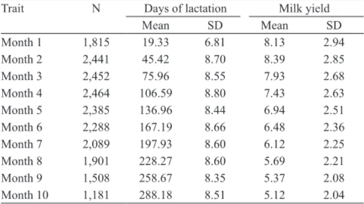
animals were excluded from the analyses. The number of records, means, standard deviations and coefficients
of variation for test‑day milk yield records, according to the monthly lactation categories, are described in Table 1.
Random regression analyses were conducted using a single‑trait model which included the random effects of animal, permanent environment and error,
and the fixed effects of contemporary group, age at
calving (linear and quadratic regressions), and mean population lactation curve. All variance and covariance
components were estimated by the restricted maximum
likelihood (REML) method, using Wombat, version 1.0 (Meyer, 2007b).
The average lactation curve was fitted by regression
on lactation days, with Legendre polynomials of the third order. Animal additive genetic and permanent
environment random effects were fitted by regressions
on lactation days, with Legendre polynomials tested for different orders, ranging from 2 to 5.
Table 1. Number of observations (N), means, and standard
deviations (SD) of milk yield and days of lactation for test‑day milk yields.
Trait N Days of lactation Milk yield
Mean SD Mean SD
Month 1 1,815 19.33 6.81 8.13 2.94
Month 2 2,441 45.42 8.70 8.39 2.85
Month 3 2,452 75.96 8.55 7.93 2.68
Month 4 2,464 106.59 8.80 7.43 2.63
Month 5 2,385 136.96 8.44 6.94 2.51
Month 6 2,288 167.19 8.66 6.48 2.36
Month 7 2,089 197.93 8.60 6.12 2.25
Month 8 1,901 228.27 8.60 5.69 2.21
Month 9 1,508 258.67 8.35 5.37 2.08
Month 10 1,181 288.18 8.51 5.12 2.04
The error covariance structure was tested as homogeneous or heterogeneous, with the latter
categorized in ten, six or four steps. For the 10‑step
models, each lactation month was considered as an error variance category. For the 6‑step and 4‑step
models, categories were defined according to the variance proximity between lactation months. Thus,
the error‑variance categories, according to lactation months, were 1, 2, 3‑5, 6, 7, and 8‑10, for the 6‑step models, and 1, 2‑5, 6‑7, and 8‑10 for the 4‑step models.
The model was (El Faro et al., 2008): y = Xb + Za + Wpe + e, in which y is a vector containing N test‑day milk yield records from Na animals; b is a vector of
solutions for the contemporary groups and the fixed
regressions for mean lactation curve (linear and quadratic), on age at calving; a is a vector of solutions for random regressions for the animal additive genetic effect; pe is a vector of random regressions for the permanent environment effect; e is a vector
of errors; X is the incidence matrix relating records to the fixed effects; and Z and W are the incidence
matrices containing orthogonal polynomials relating, respectively, the animal additive genetic effect and the permanent environment effect for lactation days.
Random effects were assumed to be normally
distributed with expectation equal to zero and the following covariance structure (El Faro et al., 2008):
y Xb V(a) = Ka A,
E a = 0 and V(pe) = Kpe INd,
pe 0 V(e) = R,
in which: Ka and Kpe are the variance and covariance
matrices, between the additive genetic coefficient and the permanent environmental regression coefficient, respectively; A is the relationship matrix of order equal
to the number of animals in the pedigree; INd is an
identity matrix of dimension Nd; and R is a diagonal matrix of residual variances. R is a diagonal matrix that
accommodate from 1 to n classes of residual variances
for the different test‑days; and σ2
a and σ2pe are the
animal additive genetic and permanent environment, respectively.
Comparisons among different models were made using Akaike’s information criterion (AIC) (Akaike,
1973), Schwarz Bayesian information criterion (BIC) (Schwarz, 1978), and the likelihood ratio test (LRT) (Wolfinger, 1993). The information criteria can be represented with the following equations: AIC = ‑2log L + 2p and BIC = ‑2log L + plog (N ‑ r), in which: p is the number of parameters in the model; N is the total number of records; r is the rank of the incidence matrix (X) for the systematic effects in the
model; and log L is the logarithm of the restricted
maximum likelihood function. The likelihood ratio
test (LRT) was used for the comparison of different
error‑variance structures (Huelsenbeck & Bull, 1996). The significance of the differences between models
was obtained using a chi‑square test of the log L values, in which the degrees of freedom equaled the number of parameters from the models.
Another analysis was also conducted on the same
data file, including all test‑day milk yield records in a finite dimensional model (FDM), for comparison with
the random regression models. The FDM were then divided into monthly classes, according to days after calving, for a total of 10 classes. In this model each monthly class was considered one trait, and the 10 traits were analyzed together. Random effects for animal additive genetic and error effects were determined
along with the fixed effects of contemporary group,
age at calving (linear and quadratic regressions) and days in milk (linear regression).
The notation for the models fitted with orthogonal
Legendre polynomials followed the pattern “Leg. Ka.Kpe.R”, in which: Ka and Kpe indicate the numbers of
random regression coefficients used to fit the additive
genetic effect and the permanent environment effect, respectively, and R indicates the number of categories for the error‑variances.
Results and Discussion
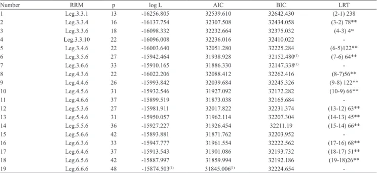
When models 1 to 4 were compared to verify the best residual variance structure, the LRT indicated that the model which considered homogenous variance
of residuals produced the worst fit, which suggests
that the residual variances have different behavior during the lactation period (Table 2). Similar results with Legendre polynomials were found by El Faro & Albuquerque (2003) for the Caracu breed, by Bignardi
et al. (2009) for the Holstein breed, and Costa et al.
(2005) for the Gyr breed. Among the models that considered different residual variance classes, the
model with six classes fit data best according to AIC, BIC and LRT. The model with six classes and that with
ten were not different according to the LRT (Table 2).
The results suggest that six heterogeneous residual variance classes are sufficient to model the residual
variance structure during lactation in this population. After choosing the residual variance structure, the models were compared by combining different orders of the polynomials for the additive genetic effect and the permanent environmental effect. When compared, it was observed that the models with the same polynomial order to model the additive genetic effect, the values of log L, AIC, and BIC improved with the increase of the polynomial order to model the permanent environmental effect. The same tendency was reported by El Faro et al. (2008) and Bignardi
et al. (2009).
The Leg.6.6.6 model attained the best values of log L and AIC, while the Leg.3.6.6 model had the best BIC. The BIC is considered a more rigorous criterion than the AIC, and tends to penalize parameterized models by selecting more parsimonious models (Meyer, 2007a). The Leg.6.6.6 model, however, contained 48 parameters, 15 more than the Leg.3.6.6 model, suggesting that the Leg.6.6.6 model is overparameterized. For the comparisons of the estimated genetic parameters, the following was
chosen: the Leg.6.6.6 model (best AIC – least
rigorous), Leg.3.6.6 model (best BIC – most rigorous), and Leg.3.5.6 model (second‑best BIC and alternative parsimonious model due to the smaller number of parameters).
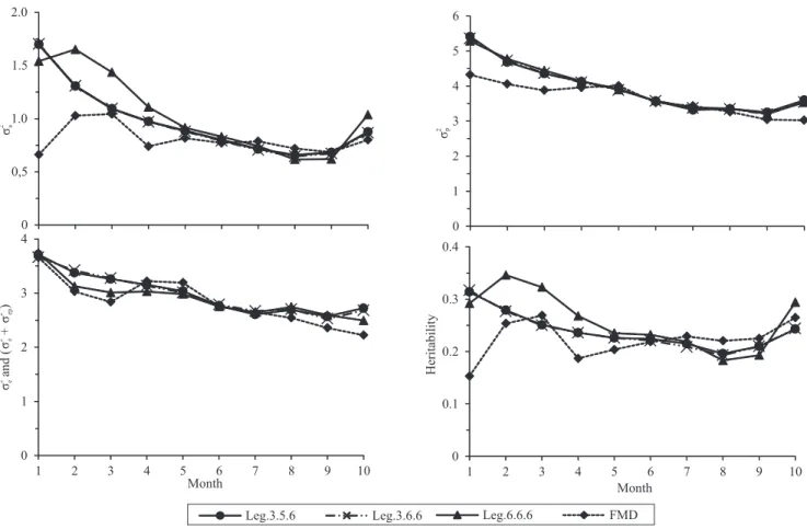
with the progress of lactation, but the RRMs showed a slight increase in the last month (Figure 1). This typical U‑shape was reported in studies by Bignardi et al.
(2009) and Miglior et al. (2009) with Holstein breed,
and by Pereira et al. (2013a) with Gyr breed. Possibly, the high estimate for the phenotypic variance, in the
first and last months, was due to the smaller number of
records in these months (in particular, in the last month not all the cows had test‑day records because of the high frequency of short lactations in the breed) (Meyer,
1999). However, according to Bohmanova et al.
(2008), the U‑shape can also be due to nonincluded factors in the model, such as the effect of pregnancy and preferential treatment between herd variations in the shape of the lactation curve.
Regarding the genetic variances, the Leg.3.5.6 and Leg.3.6.6 RRMs showed similar tendencies for the entire lactation period. The Leg.6.6.6 model showed higher estimates from the second to the fourth month of lactation than the other RRMs and FDM (which did not obey a structuring or a function in the estimation process). This result indicates that the obtained variances with Leg.6.6.6 model are possibly
overestimated, due to the overparameterization of this model. Thus, lower order polynomials are preferred to model the genetic effect by RRM, irrespectively of data size. Starting in the second half of the lactation period, the RRMs tended to show similar tendencies and values. The difference observed in the initial months for the additive genetic variance estimates possibly resulted from using a polynomial of higher order to model the additive genetic effect. This indicates that the modeling in the initial lactation phase is susceptible to variation in the polynomial’s
order, for this effect, suggesting a greater difficulty of
RRMs to model the variation in this phase. The RRMs and FDM showed similar tendencies and mutually
close estimates in the five last months of lactation,
also in the third month. However, they showed different tendencies in the initial months, with the RRMs producing estimates of higher magnitude for the genetic variance.
The estimates of the environmental variances resulting from the sum of the permanent and temporary
environmental variances (σ2
ap + σ2e or σ2e) were very
near to each other for all the RRMs and the FDM.
Table 2. Notation for each different model fitted with orthogonal Legendre polynomials (RRM), number of parameters (p),
logarithm of the restricted maximum likelihood function (log L), Akaike´s information criteria (AIC), Schwarz Bayesian information criteria (BIC), and likelihood ratio test (LRT).
Number RRM p log L AIC BIC LRT
1 Leg.3.3.1 13 ‑16256.805 32539.610 32642.430 (2‑1) 238
2 Leg.3.3.4 16 ‑16137.754 32307.508 32434.058 (3‑2) 78**
3 Leg.3.3.6 18 ‑16098.332 32232.664 32375.032 (4‑3) 4ns
4 Leg.3.3.10 22 ‑16096.008 32236.016 32410.022 ‑
5 Leg.3.4.6 22 ‑16003.640 32051.280 32225.284 (6‑5)122**
6 Leg.3.5.6 27 ‑15942.464 31938.928 32152.480(1) (7‑6) 64**
7 Leg.3.6.6 33 ‑15910.165 31886.330 32147.338(1) ‑
8 Leg.4.3.6 22 ‑16022.206 32088.412 32262.416 (8‑7)56**
9 Leg.4.4.6 26 ‑15993.842 32039.684 32245.326 (9‑8) 122**
10 Leg.4.5.6 31 ‑15932.546 31927.092 32172.282 (10‑9) 66**
11 Leg.4.6.6 37 ‑15899.519 31873.038 32165.684 ‑
12 Leg.5.3.6 27 ‑15981.911 32017.822 32231.374 (13‑12) 63**
13 Leg.5.4.6 31 ‑15950.057 31962.114 32207.304 (14‑13) 45**
14 Leg.5.5.6 36 ‑15927.227 31926.454 32211.19 (15‑14) 66**
15 Leg.5.6.6 42 ‑15893.881 31871.762 32203.952 ‑
16 Leg.6.3.6 33 ‑15947.777 31961.554 32222.562 (17‑16) 68**
17 Leg.6.4.6 37 ‑15913.543 31901.086 32193.732 (18‑17) 51**
18 Leg.6.5.6 42 ‑15887.997 31859.994 32192.186 (19‑18)26**
19 Leg.6.6.6 48 ‑15874.503(1) 31845.006(1) 32224.654 ‑
(1)Values indicate the best models based on log L, AIC, and BIC. nsNonsignificant. **Significant at 1% probability. Notation on RRM: Leg.K
a.Kpe.R, where
Ka and Kpe indicate the number of random regression coefficients used to fit the additive genetic effect and the permanent environment effect, respectively,
The heritability estimates obtained by the RRMs (Leg.3.5.6, Leg.3.6.6 and Leg.6.6.6) and by the FDM are shown in Figure 3. Among the three RRMs, the Leg.6.6.6 model obtained the highest estimates for heritability between the second and fourth month. In this period, this model estimated higher values for the additive genetic variances, probably due to the higher order of the polynomial utilized to model the additive genetic effect. The heritability estimates obtained by
the TDMO ranged from 0.15 (first month) to 0.27 (third
month), and the estimates in the initial lactation phase were lower than those obtained by the RRMs. These heritability estimates are similar to those obtained by Santos et al. (2013b) for the Guzerat breed, and by Ledic et al. 2002 for the Gyr breed, which ranged from 0.16 to 0.24 and from 0.14 to 0.24, respectively. However, Herrera et al. (2008) found the highest heritability estimates, from 0.14 to 0.34 for Gyr breed, while Bignardi et al. (2008) found the lower estimates,
which ranged from 0.07 to 0.19 for the Holstein breed.
The heritability estimates obtained by the Leg.3.5.6 and Leg.3.6.6 models were very near to each other,
from 0.32 (first month) to 0.19 (eighth month), while
for the Leg.6.6.6 model the heritability estimates varied from 0.35 (second month) to 0.18 (eighth month). Possibly, the high heritability estimates obtained by the RRMs in the initial months were
due to the difficulty of modeling this period together
with the lower number of records in these months. The heritability increase in the estimates, in the last month, can be attributed only to the lower number of records in this month, since the estimates obtained by the FDM, which do not use covariance functions, were also higher in this period. Some authors worked with Legendre polynomials and reported the same tendency of the estimates (El Faro & Albuquerque 2003). However, these authors attributed the results,
at the end of lactation, to both the difficulty of fitting
the Legendre polynomials and to the lower number of records.
Figure 1. Genetic (σ2
a), phenotypic (σ2p), and residual σ2e or (σ2pe +σ2e )variances, and heritability estimated by Leg.3.5.6,
The magnitude of the heritability estimates found in the present study is similar to those reported by Olori
et al. (1999), Cobuci et al. (2005), and Bignardi et al. (2009) for the Holstein breed. Similar results (0.20 to
0.33) were found by Santos et al. (2013a), who used RRM with parametric functions for Guzerat breed. When RRMs were used with parametric functions in Gyr dairy cows, Herrera et al. (2008) found similar estimates to those found here. Also Pereira et al. (2010) observed the similar estimates as the ones of the present
study, but in a lager range (0.09 to 0.33). Costa et al.
(2005), using Legendre polynomials for the Gyr breed, found higher heritability values, which ranged from 0.71, at the start, to 0.21 at the end of lactation, while Pereira et al. (2013a, 2013b) found lower estimates,
which ranged from 0.12 to 0.24 and from 0.12 to 0.26, respectively. These last authors used Spline function for estimating heritabilities, which ranged from 0.16
to 0.29. El Faro et al. (2008) and Araújo et al. (2006)
employed RRMs for Caracu breed and Holstein breed, respectively, and reported heritability estimates at the end of lactation lower than those obtained in the present study. The obtained heritability estimates were of medium magnitude and are consistent to those of the literature, indicating the suitability of RRM for the genetic evaluation of Guzerat milk yield.
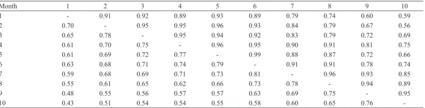
The phenotypic correlations estimated by the Leg.3.5.6, Leg.3.6.6 and Leg.6.6.6 models and the FDM were very similar, ranging from, respectively, 0.24 to 0.81, 0.26 to 0.82, 0.25 to 0.85, and 0.43 to
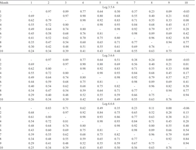
Table 3. Genetic (above the diagonal) and phenotypic (below the diagonal) correlation estimates between monthly milk yields obtained with the Leg.3.5.6, Leg.3.6.6, and Leg.6.6.6 random regression models.
Month 1 2 3 4 5 6 7 8 9 10
Leg.3.5.6
1 ‑ 0.97 0.89 0.77 0.64 0.50 0.37 0.23 0.09 ‑0.03
2 0.69 ‑ 0.97 0.90 0.80 0.68 0.55 0.40 0.21 0.02
3 0.62 0.79 ‑ 0.98 0.92 0.83 0.71 0.55 0.33 0.08
4 0.55 0.72 0.80 ‑ 0.98 0.93 0.84 0.68 0.45 0.17
5 0.49 0.64 0.74 0.80 ‑ 0.98 0.92 0.79 0.57 0.28
6 0.45 0.58 0.68 0.76 0.81 ‑ 0.98 0.89 0.69 0.42
7 0.41 0.52 0.62 0.70 0.75 0.80 ‑ 0.96 0.82 0.58
8 0.35 0.47 0.54 0.60 0.65 0.71 0.77 ‑ 0.94 0.77
9 0.30 0.42 0.48 0.51 0.55 0.61 0.69 0.76 ‑ 0.94
10 0.24 0.34 0.39 0.41 0.43 0.48 0.55 0.63 0.75 ‑
Leg.3.6.6
1 ‑ 0.97 0.89 0.77 0.64 0.51 0.38 0.24 0.09 ‑0.03
2 0.69 ‑ 0.97 0.90 0.80 0.69 0.56 0.40 0.21 0.01
3 0.62 0.80 ‑ 0.98 0.92 0.83 0.71 0.55 0.33 0.08
4 0.55 0.72 0.80 ‑ 0.98 0.93 0.84 0.68 0.45 0.17
5 0.49 0.64 0.74 0.80 ‑ 0.98 0.92 0.79 0.57 0.27
6 0.44 0.59 0.68 0.75 0.81 ‑ 0.98 0.89 0.69 0.41
7 0.40 0.54 0.62 0.68 0.75 0.82 ‑ 0.96 0.82 0.58
8 0.34 0.47 0.54 0.59 0.64 0.71 0.77 ‑ 0.94 0.77
9 0.29 0.40 0.48 0.52 0.55 0.59 0.66 0.75 ‑ 0.94
10 0.26 0.34 0.39 0.42 0.45 0.49 0.55 0.63 0.76 ‑
Leg.6.6.6
1 ‑ 0.83 0.71 0.62 0.49 0.35 0.23 0.11 0.00 ‑0.06
2 0.68 ‑ 0.97 0.92 0.84 0.75 0.65 0.52 0.28 0.15
3 0.61 0.80 ‑ 0.98 0.93 0.86 0.77 0.63 0.38 0.21
4 0.54 0.72 0.81 ‑ 0.98 0.93 0.84 0.71 0.45 0.28
5 0.48 0.64 0.74 0.80 ‑ 0.98 0.92 0.80 0.55 0.40
6 0.43 0.60 0.69 0.75 0.81 ‑ 0.98 0.89 0.66 0.54
7 0.39 0.55 0.62 0.68 0.75 0.82 ‑ 0.96 0.79 0.69
8 0.34 0.48 0.55 0.59 0.65 0.71 0.77 ‑ 0.92 0.84
9 0.29 0.41 0.48 0.52 0.55 0.59 0.67 0.75 ‑ 0.94
0.81, with higher values obtained between adjacent records, in the middle of lactation, and smaller ones in
the first and last test‑day records (Tables 3 and 4).
The genetic correlation estimates obtained with the RRMs were high and near the unity for the adjacent records, with the values declining as the interval between the test‑day records increased (Tables 3). The same tendency was reported by Bignardi et al.
(2009) for the Holstein breed, by Kettunen et al.
(2000) for the Ayrshire breed, by Herrera et al. (2008), and Pereira et al. (2013b) for the Gyr breed, and Santos et al. (2013a) for the Guzerat breed, all of them using parametric function. The three RRMs (Leg.3.5.6, Leg.3.6.6 and Leg.6.6.6) showed negative genetic correlation estimates between milk yield in
the first and in the last test‑day records, but of small
magnitudes.
The Leg.6.6.6 model tended to produce lower genetic
correlation estimates for milk yield, between the first
lactation month and the other months than did the other RRMs, obtaining a negative value near zero (‑0.003)
for the genetic correlation estimate between the first
and ninth month. Like heritability, the negative genetic
correlation estimates can be attributed to the difficulty
of RRMs to model test‑day milk yield at the beginning and end of lactation (because of the smaller number of records), since the estimate between the TDMY at the start and end of lactation obtained by the FDM was
positive and moderate in magnitude (0.59) (Table 4).
Even with this difficulty, the estimated genetic
correlations were of low magnitude and close to
zero, so that the use of RRM would not cause
major problems for different stages of lactation by
correlated response to selection for any test‑day
milk yield.
Negative correlations were also reportedby El Faro et al. (2008) and Bignardi et al. (2009)
using Legendre polynomials. Pereira et al. (2013b), using Legendre polynomials for Gyr dairy cows, found estimates of additive genetic correlations between
daily milk yields closed to 0.99 between adjacent
test days, decreasing to about 0.40 between records obtained at the beginning and at the end of lactation. When the parametric function was used in Gyr data, Herrera et al. (2008) did not estimate negative genetic correlations, while Pereira et al. (2010) reported negative genetic correlations between test‑day records at the beginning and at the end of lactation. For Guzerat breed, Santos et al. (2013a) found ‑0.15 and ‑0.03 for genetic correlation between records at the beginning and at the end of lactation, with Wilmink and Ali & Schaeffer function respectively. However, Santos et al. (2013b), using a multi‑trait model, estimated values
which ranged from 0.91 to 0.56 between all monthly
milk yields.
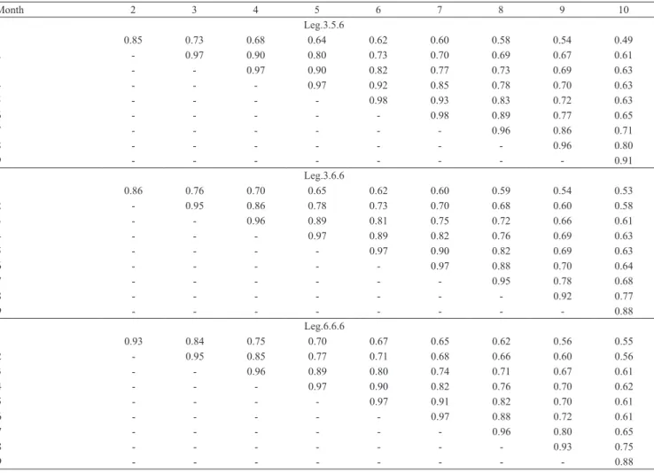
The permanent environmental correlations estimated by the RRMs were near to each other, with the Leg.6.6.6 model tending to show slightly higher estimates for the
correlations between milk yields in the first month and
the other months than the other models (Tables 5).
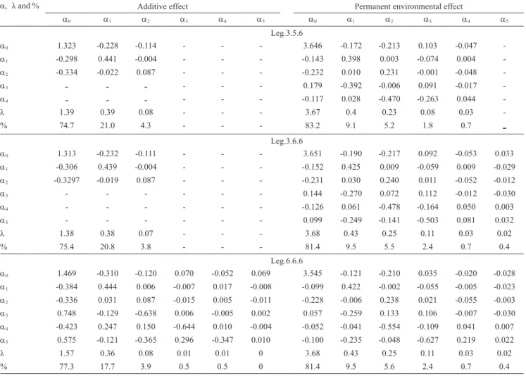
The correlations among the regression coefficients
for the additive genetic and permanent environmental effects were small and very similar for the three RRMs
(Table 6). For all the RRMs, the coefficient matrix
eigenvalues for the permanent environmental effects were higher than those for the additive genetic effects. This indicates that the polynomial orders used to model
Table 4. Genetic (above the diagonal) and phenotypic (below the diagonal) correlation estimates between monthly milk yields obtained with the finite dimensional model (FDM).
Month 1 2 3 4 5 6 7 8 9 10
1 ‑ 0.91 0.92 0.89 0.93 0.89 0.79 0.74 0.60 0.59
2 0.70 ‑ 0.95 0.95 0.96 0.93 0.84 0.79 0.67 0.56
3 0.65 0.78 ‑ 0.95 0.94 0.92 0.83 0.79 0.72 0.69
4 0.61 0.70 0.75 ‑ 0.96 0.95 0.90 0.91 0.81 0.75
5 0.61 0.69 0.72 0.77 ‑ 0.99 0.88 0.87 0.72 0.66
6 0.63 0.68 0.71 0.74 0.79 ‑ 0.91 0.91 0.78 0.74
7 0.59 0.68 0.69 0.71 0.73 0.81 ‑ 0.96 0.93 0.85
8 0.55 0.61 0.65 0.62 0.66 0.73 0.78 ‑ 0.94 0.89
9 0.48 0.55 0.56 0.57 0.57 0.63 0.69 0.75 ‑ 0.95
the permanent environmental effect should be higher than those used to model the additive genetic effect (El Faro et al., 2008). These results are similar to those found by Brotherstone et al. (2000) for the Hosltein
breed, and by El Faro et al. (2008) studying Caracu cows.
For the additive genetic effect – obtained with the Leg.6.6.6 (Table 6), Leg.5.6.6 and Leg.4.6.6 models –,
the last eigenvalue of the random regression coefficient matrix was equal to zero, indicating that the addition of
these parameters (referring to Ka) did not contribute to
the total variation of this effect. This result suggests
that a third‑order polynomial is sufficient to model
the additive genetic effect for the data in the present study, as also observed in other studies (Olori et al.,
1999; Kettunen et al., 2000; Takma & Akbas, 2009).
The eigenvalue magnitudes of the random regression
coefficients for the additive genetic effect obtained in the three models were near to each other, with the first eigenvalue representing more than 75% of the total
variation. For the permanent environmental effect, the sum of the three eigenvalues, obtained with the three
RRMs, was also similar, representing 96% of the total
variation of this effect.
The eigenfunctions were estimated from
eigenvectors of the random regression coefficient matrix for the additive genetic effect. The Leg.3.5.6 had
the same pattern for the entire period as the Leg.3.6.6.
The first eigenfunction was positive for the entire
lactation period, tending to decline slightly at the end
of the period (Druet et al., 2003). Olori et al. (1999),
Araújo et al. (2006) and El Faro et al. (2008) also
reported that the first eigenfunction was positive and
constant during the entire lactation period, indicating
Table 5. Permanent environmental correlation estimates between monthly milk yields obtained with the Leg.3.5.6, Leg.3.6.6 and Leg.6.6.6 random regression models.
Month 2 3 4 5 6 7 8 9 10
Leg.3.5.6
1 0.85 0.73 0.68 0.64 0.62 0.60 0.58 0.54 0.49
2 ‑ 0.97 0.90 0.80 0.73 0.70 0.69 0.67 0.61
3 ‑ ‑ 0.97 0.90 0.82 0.77 0.73 0.69 0.63
4 ‑ ‑ ‑ 0.97 0.92 0.85 0.78 0.70 0.63
5 ‑ ‑ ‑ ‑ 0.98 0.93 0.83 0.72 0.63
6 ‑ ‑ ‑ ‑ ‑ 0.98 0.89 0.77 0.65
7 ‑ ‑ ‑ ‑ ‑ ‑ 0.96 0.86 0.71
8 ‑ ‑ ‑ ‑ ‑ ‑ ‑ 0.96 0.80
9 ‑ ‑ ‑ ‑ ‑ ‑ ‑ ‑ 0.91
Leg.3.6.6
1 0.86 0.76 0.70 0.65 0.62 0.60 0.59 0.54 0.53
2 ‑ 0.95 0.86 0.78 0.73 0.70 0.68 0.60 0.58
3 ‑ ‑ 0.96 0.89 0.81 0.75 0.72 0.66 0.61
4 ‑ ‑ ‑ 0.97 0.89 0.82 0.76 0.69 0.63
5 ‑ ‑ ‑ ‑ 0.97 0.90 0.82 0.69 0.63
6 ‑ ‑ ‑ ‑ ‑ 0.97 0.88 0.70 0.64
7 ‑ ‑ ‑ ‑ ‑ ‑ 0.95 0.78 0.68
8 ‑ ‑ ‑ ‑ ‑ ‑ ‑ 0.92 0.77
9 ‑ ‑ ‑ ‑ ‑ ‑ ‑ ‑ 0.88
Leg.6.6.6
1 0.93 0.84 0.75 0.70 0.67 0.65 0.62 0.56 0.55
2 ‑ 0.95 0.85 0.77 0.71 0.68 0.66 0.60 0.56
3 ‑ ‑ 0.96 0.89 0.80 0.74 0.71 0.67 0.61
4 ‑ ‑ ‑ 0.97 0.90 0.82 0.76 0.70 0.62
5 ‑ ‑ ‑ ‑ 0.97 0.91 0.82 0.70 0.61
6 ‑ ‑ ‑ ‑ ‑ 0.97 0.88 0.72 0.61
7 ‑ ‑ ‑ ‑ ‑ ‑ 0.96 0.80 0.65
8 ‑ ‑ ‑ ‑ ‑ ‑ ‑ 0.93 0.75
that practically the same genetic factors influence
the genetic variance throughout the lactation period.
The second eigenfunction was negative until the fifth
month and positive thereafter, and the corresponding
eigenvalue explained 21% of the total variation. This
contrast indicates that the eingenfunction is possibly related to the persistence of lactation (Olori et al.,
1999).
The rank correlation between the sires breeding values predicted by the Leg.3.5.6 and Leg.3.6.6 was
very high (99.88%), while by Leg.3.5.6, Leg.3.6.6, and Leg.6.6.6 values were around 90%. This result
suggests that sires would be ranked practically in the same order if Leg.3.5.6 or Leg.3.6.6 were applied for genetic evaluations. However, despite correlations are also high by Leg.6.6.6, they indicated that there
are some changes in the rank between bulls in relation to other evaluated models. This small difference is
possibly due to overfitting of the genetic effect by
this model.
Conclusions
1. It is necessary to consider the heterogeneity of the
residual variances to fit test‑day milk yield curves for
the Guzerat breed.
2. The random regression model using a second‑order Legendre polynomial for the additive
genetic effect, and a fifth‑order polynomial for the permanent environmental effect, with six residual variance classes, is the most suitable to fit the data.
Table 6. Estimates of variances (diagonal), covariance (below the diagonal), and correlations (above the diagonal) between random regression coefficients and eigenvalues (λ), and percentage explanation (%) of the coefficient matrix obtained by Leg.3.5.6, Leg.3.6.6, and Leg.6.6.6 random regression models.
a, λand % Additive effect Permanent environmental effect
a0 a1 a2 a3 a4 a5 a0 a1 a2 a3 a4 a5
Leg.3.5.6
a0 1.323 ‑0.228 ‑0.114 ‑ ‑ ‑ 3.646 ‑0.172 ‑0.213 0.103 ‑0.047 ‑
a1 ‑0.298 0.441 ‑0.004 ‑ ‑ ‑ ‑0.143 0.398 0.003 ‑0.074 0.004 ‑
a2 ‑0.334 ‑0.022 0.087 ‑ ‑ ‑ ‑0.232 0.010 0.231 ‑0.001 ‑0.048 ‑
a3 ‑ ‑ ‑ ‑ ‑ ‑ 0.179 ‑0.392 ‑0.006 0.091 ‑0.017 ‑
a4 ‑ ‑ ‑ ‑ ‑ ‑ ‑0.117 0.028 ‑0.470 ‑0.263 0.044 ‑
λ 1.39 0.39 0.08 ‑ ‑ ‑ 3.67 0.4 0.23 0.08 0.03 ‑
% 74.7 21.0 4.3 ‑ ‑ ‑ 83.2 9.1 5.2 1.8 0.7
‑
Leg.3.6.6
a0 1.313 ‑0.232 ‑0.111 ‑ ‑ ‑ 3.651 ‑0.190 ‑0.217 0.092 ‑0.053 0.033
a1 ‑0.306 0.439 ‑0.004 ‑ ‑ ‑ ‑0.152 0.425 0.009 ‑0.059 0.009 ‑0.029
a2 ‑0.3297 ‑0.019 0.087 ‑ ‑ ‑ ‑0.231 0.030 0.240 0.011 ‑0.052 ‑0.012
a3 ‑ ‑ ‑ ‑ ‑ ‑ 0.144 ‑0.270 0.072 0.112 ‑0.012 ‑0.030
a4 ‑ ‑ ‑ ‑ ‑ ‑ ‑0.126 0.061 ‑0.478 ‑0.164 0.050 0.003
a5 ‑ ‑ ‑ ‑ ‑ ‑ 0.099 ‑0.249 ‑0.141 ‑0.503 0.081 0.032
λ 1.38 0.38 0.07 ‑ ‑ ‑ 3.68 0.43 0.25 0.11 0.03 0.02
% 75.4 20.8 3.8 ‑ ‑ ‑ 81.4 9.5 5.5 2.4 0.7 0.4
Leg.6.6.6
a0 1.469 ‑0.310 ‑0.120 0.070 ‑0.052 0.069 3.545 ‑0.121 ‑0.210 0.035 ‑0.020 ‑0.028
a1 ‑0.384 0.444 0.006 ‑0.007 0.017 ‑0.008 ‑0.099 0.422 ‑0.002 ‑0.055 ‑0.005 ‑0.023
a2 ‑0.336 0.031 0.087 ‑0.015 0.005 ‑0.011 ‑0.228 ‑0.006 0.238 0.021 ‑0.055 ‑0.003
a3 0.748 ‑0.129 ‑0.638 0.006 ‑0.005 0.002 0.057 ‑0.259 0.133 0.106 ‑0.007 ‑0.030
a4 ‑0.423 0.247 0.150 ‑0.644 0.010 ‑0.004 ‑0.052 ‑0.041 ‑0.554 ‑0.109 0.041 0.007
a5 0.575 ‑0.121 ‑0.365 0.296 ‑0.347 0.010 ‑0.100 ‑0.235 ‑0.048 ‑0.627 0.219 0.022
λ 1.57 0.36 0.08 0.01 0.01 0 3.68 0.43 0.25 0.11 0.03 0.02
3. The random regression model using a second‑order Legendre polynomial, for the genetic effect, and a fourth‑order one, for the permanent environmental
effect is sufficient to obtain similar results from the model with the fifth‑order polynomial for the
permanent environmental effect.
Acknowledgements
To Conselho Nacional de Desenvolvimento Científico e Tecnológico (CNPq) and to Fundação
de Amparo à Pesquisa do Estado de Minas Gerais
(Fapemig), for financial support.
References
AKAIKE, H. Information theory and an extension of the maximum likelihood principle. In: INTERNATIONAL SYMPOSIUM ON INFORMATION THEORY, 2., 1973, Budapest. Proceedings. Budapest: Akademiai Kiado, 1973. p.267‑281.
ARAúJO, C.V. de; TORRES, R. de A.; COSTA, C.N.; TORRES FILHO, R. de A.; ARAúJO, S.I.; LOPES, P.S.; REGAZZI, A.J.; PEREIRA, C.S.; SARMENTO, J.L.R. Uso de modelos de regressão aleatória para descrever a variação genética da produção de leite na raça Holandesa. Revista Brasileira de Zootecnia,v.35, p.975‑981, 2006. DOI: 10.1590/S1516‑35982006000400005. BIGNARDI, A.B.; EL FARO, L.; ALBUQUERQUE, L.G. de; CARDOSO, V.L.; MACHADO, P.F. Modelos de dimensão finita para a estimação de parâmetros genéticos para a produção de leite de primeiras lactações de vacas da raça Holandesa.
Ciência Rural, v.38, p.1705‑1710, 2008. DOI: 10.1590/
S0103‑84782008000600033.
BIGNARDI, A.B.; EL FARO, L.; CARDOSO, V.L.; MACHADO, P.F.; ALBUQUERQUE, L.G. Random regression models to estimate test‑day milk yield genetic parameters in Holstein cows in Southeastern Brazil. Livestock Science, v.123, p.1‑7, 2009. DOI:
10.1016/j.livsci.2008.09.021.
BOHMANOVA, J.; MIGLIOR, F.; JAMROZIK, J.; MISZTAL, I.; SULLIVAN, P.G. Comparison of random regression models with Legendre polynomials and linear splines for production traits and somatic cell score of Canadian Holstein cows. Journal of Dairy Science, v.91, p.3627‑3638, 2008. DOI: 10.3168/jds.2007‑0945.
BROTHERSTONE, S.; WHITE, I.M.S.; MEYER, K. Genetic modelling of daily milk yield using orthogonal polynomials and parametric curves. Animal Science, v.70, p.407‑415, 2000.
COBUCI, J.A.; EUCLYDES, R.F.; LOPES, P.S.; COSTA, C.N.; TORRES, R.A.; PEREIRA, C.S. Estimation of genetic parameters for test‑day milk in Holstein cows using a random regression model. Genetics and Molecular Biology, v.28, p.75‑83, 2005. DOI: 10.1590/S1415‑47572005000100013.
COSTA, C.N.; MELO, C.M.R. de; MACHADO, C.H.C.; FREITAS, A.F. de; PACKER, I.U.; COBUCI, J. de A. Parâmetros genéticos para a produção de leite de controles individuais de vacas da raça
Gir Leiteiro estimados com modelos de repetibilidade e regressão aleatória. Revista Brasileira de Zootecnia, v.34, p.1519‑1530,
2005. DOI: 10.1590/S1516‑35982005000500012.
DRUET, T.; JAFFRÉZIC, F.; BOICHARD, D.; DUCROCV, V. Modeling lactation curves and estimation of genetic parameters for first lactation test‑day records or French Holstein cows. Journal of Dairy Science, v.86, p.2480‑2490, 2003. DOI: 10.3168/jds.
S0022‑0302(03)73842‑9.
EGITO, A.A.; MARIANTE, A.S.; ALBUQUERQUE, M.S.M. Programa brasileiro de conservação de recursos genéticos animais.
Archivos de Zootecnia, v.51, p.39‑52, 2002.
EL FARO, L.; ALBUQUERQUE, L.G. de. Estimação de parâmetros genéticos para produção de leite no dia do controle e produção acumulada até 305 dias, para as primeiras lactações de vacas da raça Caracu. Revista Brasileira de Zootecnia, v.32, p.284‑264, 2003. DOI: 10.1590/S1516‑35982003000200006. EL FARO, L.; CARDOSO, V.L.; ALBUQUERQUE, L.G. de. Variance component estimates applying random regression models for test‑day milk yield in Caracu heifers (Bos taurus Artiodactyla, Bovidae). Genetics and Molecular Biology, v.31, p.665‑673, 2008. DOI: 10.1590/S1415‑47572008000400011.
HERRERA, L.G.G.; EL FARO, L.; ALBUQUERQUE, L.G. de; TONHATI, H.; MACHADO, C.H.C. Estimativas de parâmetros genéticos para a produção de leite e persistência da lactação em vacas Gir, aplicando modelos de regressão aleatória. Revista Brasileira de Zootecnia, v.37, p.1584‑1594, 2008. DOI: 10.1590/
S1516‑35982008000900009.
HERRERA, L.G.G.; EL FARO, L.; ALBUQUERQUE, L.G. de; TONHATI, H.; MACHADO, C.H.C. Parâmetros genéticos para produção de leite no dia do controle e para produção de leite até 305 dias nas primeiras lactações de vacas da raça Gir. Revista Brasileira de Zootecnia, v.37, p.1774‑1780, 2008. DOI: 10.1590/
S1516‑35982008001000009.
HUELSENBECK, J.P.; BULL, J.J. A likelihood ratio test to detect conflicting phylogenetic signal. Systematic Biology, v.45, p.92‑98,
1996. DOI: 10.1093/sysbio/45.1.92.
JAMROZIK, J.; SCHAEFFER, L.R. Estimates of genetic parameters for a test day model with random regressions for yield traits of first lactation Holsteins. Journal of Dairy Science v.80, p.762‑770, 1997. DOI: 10.3168/jds.S0022‑0302(97)75996‑4. KETTUNEN, A.; MäNTYSAARI, E.A.; PÖSÖ, J. Estimation of genetic parameters daily milk yield of primiparous Ayrshire cows by random regression “test‑day” models. Livestock Production Science, v.66, p.251‑261, 2000. DOI: 10.1016/
S0301‑6226(00)00166‑4.
KIRKPATRICK, M.; HECKMAN, N. A quantitative genetic model for growth, shape, reaction norms, and other infinite‑dimensional characters. Journal of Mathematical Biology, v.27, p.429‑450,
1989. DOI: 10.1007/BF00290638.
MEYER, K. Estimates of genetic and phenotypic covariance functions for postweaning growth and mature weight of beef cows.
Journal of Animal Breeding Genetics, v.116, p.181‑205, 1999.
DOI: 10.1046/j.1439‑0388.1999.00193.x.
Breeding Genetics,v.124, p.50‑64, 2007a. DOI: 10.1111/j.1439‑0 388.2007.00637.x.
MEYER, K. WOMBAT: a tool for mixed model analyses in quantitative genetics by restricted maximum likelihood (REML).
Journal of Zhejiang University. Science B, v.8, p.815‑821, 2007b. DOI: 10.1631/jzus.2007.B0815.
MEYER, K.; HILL, W.G. Estimation of genetic and phenotypic covariance functions for longitudinal or ‘repeated’ records by restricted maximum likelihood. Livestock Production Science, v.47, p.185‑200, 1997. DOI: 10.1016/S0301‑6226(96)01414‑5. MIGLIOR, F.; GONG, W.; WANG, Y.; KISTEMAKER, G.J.; SEWALEM, A.; JAMROZIK, J. Short communication: genetic parameters of production traits in Chinese Holsteins using a random regression test‑day model. Journal of Dairy Science, v.92, p.4697‑4706, 2009. DOI: 10.3168/jds.2009‑2212.
MRODE, R.A. Linear models for the prediction of animal breeding values. 2nd ed. Oxfordshire: CABI Publishing, 2005.
340p.
OLORI, V.E.; HILL, W.G.; MCGUIRK, B.J.; BROTHERSTONE, S. Estimating variance components for test day milk records by restricted maximum likelihood with a random regression animal model. Livestock Production Science, v.61, p.53‑63, 1999. DOI:
10.1016/S0301‑6226(99)00052‑4.
PEIXOTO, M.G.C.D.; POGGIAN, C.F.; VERNEQUE, R.S.; EGITO, A.A.; CARVALHO, M.R.S.; PENNA, V.M.; BERGMANN, J.A.G.; VICCINI, L.F.; MACHADO, M.A. Genetic basis and inbreeding in the Brazilian Guzerat (Bos indicus) subpopulation selected for milk production. Livestock Science, v.131, p.168‑174, 2010. DOI: 10.1016/j.livsci.2010.03.015.
PEREIRA, R.J.; AYRES, D.R.; EL FARO, L.; VERCESI FILHO, A.E.; VERNEQUE, R. S.; ALBUQUERQUE, L.G. Genetic parameters for production traits of dairy Gyr (Bos indicus) x Holstein cattle estimated with a random regression model.
Livestock Science, v.158, p.24‑31, 2013a. DOI: 10.1016/j.
livsci.2013.10.003.
PEREIRA, R.J.; BIGNARDI, A.B.; EL FARO, L.; VERNEQUE, R.S.; VERCESI FILHO, A.E.; ALBUQUERQUE, L.G. Random regression models using Legendre polynomials or linear splines for test‑day milk yield of dairy Gyr (Bos indicus) cattle. Journal
of Dairy Science, v.96, p.565‑574, 2013b. DOI: 10.3168/
jds.2011‑5051.
PEREIRA, R.J.; LOPES, P.S.; VERNEQUE, R. da S.; SANTANA JÚNIOR, M.L.; LAGROTTA, M.R.; TORRES, R. de A. Funções de covariância para produção de leite no dia do controle em bovinos Gir leiteiro. Pesquisa Agropecuária Brasileira, v.45, p.1303‑1311, 2010. DOI: 10.1590/S0100‑204X2010001100011. POOL, M.H.; MEUWISSEN, T.H.E. Reduction of the number of parameters needed for a polynomial random regression test day model. Livestock Production Science, v.64, p.133‑145, 2000. DOI: 10.1016/S0301‑6226(99)00166‑9.
SANTOS, D.J.A.; PEIXOTO, M.G.C.D.; ASPILCUETA BORQUIS, R.R.; VERNEQUE, R.S.; PANETTO, J.C.C.; TONHATI, H. Comparison of random regression models to estimate genetic parameters for milk production in Guzerat (Bos indicus) cows. Genetics and Molecular Research, v.12, p.143‑153, 2013a. DOI: 10.4238/2013.January.24.6.
SANTOS, D.J.A.; PEIXOTO, M.G.C.D.; BORQUIS, R.R.A.; VERNEQUE, R.S.; PANETTO, J.C.C.; TONHATI, H. Genetic parameters for test‑day milk yield, 305‑day milk yield, and lactation length in Guzerat cows. Livestock Science, v.152, p.114‑153, 2013b. DOI: 10.1016/j.livsci.2012.12.012.
SCHAEFFER, L.R.; JAMROZIK, J. Random regression models: a longitudinal perspective. Journal of Animal Breeding and Genetics, v.125, p.145‑146, 2008. DOI: 10.1111/j.1439‑0388.200
8.00748.x.
SCHWARZ, G. Estimating the dimension of a model. The Annals of Statistics, v.6, p.461‑464, 1978. DOI: 10.1214/
aos/1176344136.
TAKMA, C.; AKBAS, Y. Heterogeneity of residual variances of test day milk yields estimated by random regression model in Turkish Holsteins. Journal of Animal and Veterinary Advances, v.8, p.782‑787, 2009.
WERF, J. van der; SCHAEFFER, L.R. Random regression in animal breeding. Guelph: University of Guelph, 1997. 50p.
WOLFINGER, R. Covariance structure selection in general mixed models. Communications in Statistics, v.22, p.1079‑1106, 1993.
DOI: 10.1080/03610919308813143.