Caries detection in panoramic dental x-ray images

(1)

João Paulo Ribeiro de Oliveira

Caries Detection in Panoramic Dental

X-ray Images

Universidade da Beira Interior

Departamento de Informática

(2)

João Paulo Ribeiro de Oliveira

Caries Detection in Panoramic Dental

X-ray Images

Thesis submitted to the Department of Computer Science for the fulfilment of the requirements for the degree of Master in Science made under the supervision of Doctor Hugo C. Proença, Assistant Professor at the Department of Computer Science of University of Beira Interior, Covilhã, Portugal

Universidade da Beira Interior Departamento de Informática

(3)

Acknowledgements

I leave this section the special thank you to everyone who in some way contributed to the final result of this document.

First of all a special thanks to Professor Dr. Hugo Proença, for all the support and all the wisdom available to the achieving of this dissertation. Note also that always showed the willingness to answer questions and discuss the different decisions to make for the different steps of our dissertation. To Professor Dr. Hugo Proença a special and honorable thanks.

Special thanks also to Dr. Rui Conceição because without him it would not be possible the completion of this dissertation. Also thanks the availability provided to obtain an opinion from a specialist about certain decisions taken in our dissertation. To my closest family, my mother Ana Bela Oliveira, my brothers José Miguel Oliveira and Luís Gonçalo Oliveira and to my grandmother Beatriz Ferreira. For all the support and strength throughout these years of university.

To my special friends Joel Carvalho, Orlando Pereira and Sílvio Filipe.

A word of appreciation to the research group of Soft Computing and Image Analysis Lab (Socia Lab.) for all the meetings where we discuss the work of all the members.

I thank my colleagues in the Socia Lab., Release and NMCG throughout the companionship and mutual provided in different times of the day. Leave a special word of appreciation to Gil Melfe.

The last but not the least to my beautiful girlfriend, Ana Teresa de Jesus Pereira. Which throughout all these years was my shelter and in the same time my fountain of strength. Thank you.

Thanks to all the people who were not particularly mentioned but still had an important role in my education.

(4)

(5)

List of Figures

1.1 The Outline of our developed work. . . 6

2.1 All cases of the fitting curve, image extracted from [10]. . . 21

3.1 Picture of the Orthoralix 9200 DDE X-ray camera. . . 24

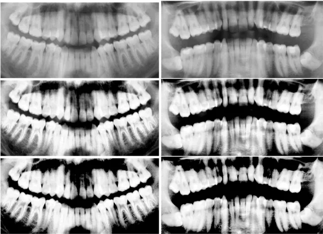
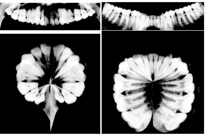
3.2 Examples of images of the Dental X-ray data set. . . 26

3.3 Number of images concerning the quantity of teeth per mouth. . . . 27

3.4 Average sizes and corresponding confidence intervals, regarding the type of teeth. . . 28

4.1 Four lengths extracted of our images data-set. . . 32

4.2 Histogram of the Ri values. . . 32

4.3 Some results for the Region of Interest (ROI) definition. . . 33

4.4 Horizontal Projection of the intensities, for our starting point. . . 34

4.5 Results of the polynomial least squares fitting. . . 35

4.6 Results of the polynomial least squares fitting in images with accen-tuated missing teeth area. . . 36

5.1 Example of the minimum intensities for one input image. . . 38

5.2 Example of our method 1 results. . . 40

5.3 Example of failure in the teeth gap valley detection of our method 1. 41 5.4 Example one of the top and bottom hat transform. . . 43

5.5 Example two of the top and bottom hat transform. . . 44

5.6 Example of the Jaws division. . . 45 5.7 The resulting polar coordinates transformation for each separated jaw. 47

(10)

5.8 The example mask of our initialization for the active contour method. 48 5.9 Output example of the active contour without edges method, applied

in each jaw. . . 49 5.10 The distance to the center of the lower jaw and the corresponding

0.10 ∗ h cut. . . 52 5.11 The distance to the center of the upper jaw and the correspond 0.10∗h

cut. . . 53 5.12 The gaussian filter for the convolution with the distance vector. . . . 54 5.13 Convolution applied to the upper and lower jaw distance vector,

based on the filter in 5.12. . . 55 5.14 Output of the minimums extraction step, applied to the upper a lower

jaw, respectively. . . 56 5.15 An example of our method 2 for the teeth gap valley detection. . . . 57

6.1 Example of our input images for the tooth segmentation stage. . . 62 6.2 Example of our input images for the tooth segmentation stage after

the Top and Bottom Hat transformation. . . 62 6.3 Example images of the top and bottom hat transform. . . 63 6.4 Some mask examples of our initialization for the active contour method. 64 6.5 Examples of the active contours method applied to our input images. 65 6.6 Examples of the active contours method applied to our input images

with overlap teeth. . . 65 6.7 Examples of the active contours method applied to our input images

with extra noise present in the output image. . . 65 6.8 The main types of connectivity analysis, image extracted from [35]. . 75 6.9 The order that our pixels are visited, this figure is extracted from [35]. 76

7.1 Results containing extra noise from the ROI definition stage. . . 89 7.2 Example of cutting teeth from the ROI definition stage. . . 89 7.3 Results where some teeth are overlapped by the polynomial fitting

in the Jaws Partition stage. . . 91

(11)

7.4 Examples of output images with the presence of teeth overlap seg-mentation. . . 95 7.5 Examples of output images with the presence of extra noise. . . 95 7.6 Receiver Operating Characteristic (ROC) for the Artificial Neural

Network (ANN) classifier for the normalized test set between [0, 1] test and training set. . . 101 7.7 ROC for the ANN classifier for the normalized test set between [0, 1]

after the appliance of the Principal Component Analysis (PCA) for a 99% variance coverage. . . 101

(12)

(13)

List of Tables

3.1 Properties of the Orthoralix 9200 imaging device. . . 25 3.2 Statistic date retrieve of our images data-set. . . 29

6.1 Results from appliance of the PCA in our training set. . . 84

7.1 Results of our method stages up to the Dental Caries Detection. . . . 88 7.2 Confusion matrix for the ANN classifier after the PCA appliance for

95% variance covering. . . 98 7.3 Confusion matrix for the Support Vector Machine (SVM) classifier

after the PCA appliance for 95% variance covering. . . 99 7.4 Confusion matrix for the Naive Bayes classifier after the PCA

appli-ance for 95% variappli-ance covering. . . 99 7.5 Confusion matrix for the ANN classifier for the normalized test set

between [0, 1] test and training set. . . 100 7.6 Confusion matrix for the ANN classifier for the normalized test set

between [0, 1] after the appliance of the PCA for a 99% variance coverage. . . 102 7.7 Confusion matrix for the SVM classifier for the test set normalized

between [0, 1] after the appliance of the PCA for a 99% variance coverage. . . 102 7.8 Confusion matrix for the Naive Bayes classifier for the test set

normal-ized between [0, 1] after the appliance of the PCA for a 99% variance coverage. . . 103

8.1 Resume table of our results accuracy for each method stage. . . 108

(14)

(15)

Acronym

ROI Region of Interest

Socia Lab. Soft Computing and Image Analysis Lab

AM Ante-Mortem

PM Post-Mortem

MRI Magnetic Resonance Imaging

CT Computerized tomography

GVF Gradient Vector Flow

BMD Bone Mineral Density

PCA Principal Component Analysis

SVM Support Vector Machine

VIPImage’09 II Eccomas Thematic Conference on Computational Vision and Medical Image Processing

FFT Fast Fourier Transform

MPP Minimum-Perimeter Polygons

IDM Inverse Difference Moment KNN K Nearest Neighborhood

NN Neural Network

ANN Artificial Neural Network

(16)

xvi ACRONYM

ROC Receiver Operating Characteristic

FPR False Positive Rate

FNR False Negative Rate

TNR True Negative Rate

TPR True Positive Rate

(17)

Chapter 1 Introduction

The detection of dental caries, in a preliminary stage are of most importance. There is a long history of dental caries. Over a million years ago, hominids such as Australopithecus suffered from cavities. Archaeological evidence shows that tooth decay is an ancient disease dating far into prehistory. Skulls dating from a million years ago through the Neolithic period show signs of caries [2]. The increase of caries during the Neolithic period may be attributed to the increase of plant foods containing carbohydrates [39]. The beginning of rice cultivation in South Asia is also believed to have caused an increase in caries.

Dental Caries, also known as dental decay or tooth decay, is defined as a disease of the hard tissues of the teeth caused by the action of microorganisms, found in plaque, on fermentable carbohydrates (principally sugars). At the individual level, dental caries is a preventable disease. Given its dynamic nature the dental caries disease, once established, can be treated or reversed prior to significant cavitation taking place. There three types of dental caries [59], the first type is the Enamel Caries, that is preceded by the formation of a microbial dental plaque. Secondly the Dentinal Caries which begins with the natural spread of the process along the natural spread of great numbers of the dentinal tubules. Thirdly the Pulpal Caries that corresponds to the root caries or root surface caries.

Primary diagnosis involves inspection of all visible tooth surfaces using a good light source, dental mirror and explorer. Dental radiographs (X-rays) may show dental caries before it is otherwise visible, particularly caries between the teeth.

(18)

2 CHAPTER 1. INTRODUCTION

Large dental caries are often apparent to the naked eye, but smaller lesions can be difficult to identify. Visual and tactile inspection along with radiographs are employed frequently among dentists. At times, caries may be difficult to detect. Bacteria can penetrate the enamel to reach dentin, but then the outer surface maybe at first site intact. These caries, sometimes referred to as "hidden caries", in the preliminary stage X-ray are the only way to detect them, despite of the visual examination of the tooth shown the enamel intact or minimally perforated. Without X-rays wouldn’t be possible to detect these problems until they had become severe and caused serious damage.

There are three main types of dental X-rays to perform the dental caries detection and other diseases [34]:

- The panoramic dental X-ray: Panoramic X-rays show a broad view of the jaws, teeth, sinuses, nasal area, and temporomandibular (jaw) joints. These X-rays do show problems such as impacted teeth, bone abnormalities, cysts, solid growths (tumors), infections, fractures and dental caries.

- The bitewing dental X-ray: Bitewing X-rays show the upper and lower back teeth and how the teeth touch each other in a single view. These X-rays are used to check for decay between the teeth and to show how well the upper and lower teeth line up. They also show bone loss when severe gum disease or a dental infection is present.

- Periapical X-rays: Periapical X-rays show the entire tooth, from the exposed crown to the end of the root and the bones that support the tooth. These X-rays are used to find dental problems below the gum line or in the jaw, such as impacted teeth, abscesses, cysts, tumors, and bone changes linked to some diseases.

1.1 Main Goal

The main goal of the work presented is to detect dental caries in panoramic dental X-ray images. Based on the panoramic input X-X-rays, our proposal is to mark infected teeth present in the image.

(19)

1.2. MOTIVATION 3

1.2 Motivation

The main motivation for this research work is the fact that is included in an area of great interest to the scientific community. Where increasingly the computer vision is become a part of our daily life, whether for security reasons as for reasons of leisure. The other major motivation is that this is an innovative work because there is not a complete case study in the literature as described in this document. In literature there are only some of the steps we implemented in our work. This work will be possible to the scientific community to be a basis for other methods or to the improvement of our method. Which method concerns the detection of dental caries in the panoramic X-ray images.

1.3 Computer Vision

Computer vision is the science e and technology that correspond to the vision of machines. As a scientific discipline, computer vision is the process to obtain information from images by building a artificial system. This images data can be presented to the system in many forms, the most popular views from a single camera, video sequence, views from multiple cameras, or multi-dimensional data from a medical scanner.

The classical problem in computer vision is that of determining whether or not the image data contains some specific object, feature, or activity. This task can normally be solved robustly and without effort by a human, but is still not satisfactorily solved in computer vision for the general case: arbitrary objects in arbitrary situations. The existing methods for dealing with this problem can at best solve it only for specific objects, such as simple geometric objects, human faces, printed or hand-written characters, or vehicles, and in specific situations, typically described in terms of well-defined illumination, background, and pose of the object relative to the camera in [15][55]. There are a variety of recognition problem, such as:

- Recognition: This problem consists in the recognition of objects that were pre-specified or learned by the system.

(20)

identify individuals, this can be fulfill by the use of the individual face, fingertips, teeth contour, etc.

- Detection: Our work fits in this recognition problem, because the main goal is to detect, in the image, regions containing dental caries. In this case the propose of capturing the images, is effectively limited for detection of dental caries.

The organization of a computer vision system is highly application dependent. Some systems are stand-alone applications which solve a specific measurement or detection problem, while other constitute a sub-system of a larger design which, for example, also contains sub-systems for control of mechanical actuators, planning, information databases, man-machine interfaces, etc. The specific implementation of a computer vision system also depends on if it’s functionality is pre-specified or if some part of it can be learned or modified during operation. There are, however, typical functions which are found in many computer vision systems [13][55][18]:

- Image Acquisition: A digital image is produced by one or several image sensors, which, besides various types of light-sensitive cameras, include range sensors, tomography devices, radar, ultra-sonic cameras, etc. Depending on the type of sensor, the resulting image data is an ordinary 2D image, a 3D volume, or an image sequence. The pixel values typically correspond to light intensity in one or several spectral bands (gray images or color images), but can also be related to various physical measures, such as depth, absorption or reflectance of sonic or electromagnetic waves, or nuclear magnetic resonance. - Pre-Processing: This stage is perform before a computer vision method can be applied to image data in order to extract some specific information, it is usually necessary to process the data in order to assure that it satisfies certain assumptions implied by the method. For example noise reduction in order to assure that is not introduce false information to the system, contrast enhancement to assure that relevant information can be detected and scale-space representation to increase relevant information in appropriate scales. - Feature Extraction: Image features at various levels of complexity are

ex-tracted from the image data. There are two types of feature extraction, the low-level that corresponds to the basic features that can be extracted automatically

(21)

1.4. BLOCK DIAGRAM 5

from an image without any shape information. And the high-level feature extraction concerns finding shapes in computer images [35].

- Detection/Segmentation: In computer vision, segmentation refers to the process of partitioning a digital image into multiple segments (sets of pixels) . The goal of segmentation is to simplify and/or change the representation of an image into something that is more meaningful and easier to analyze [57]. Image segmentation is typically used to locate objects and boundaries (lines, curves, etc.) in images. More precisely, image segmentation is the process of assigning a label to every pixel in an image such that pixels with the same label share certain visual characteristics.

- High-level processing: In this step the input is generally a data-set containing a specific object. This is based on the features that describe the region. For example, in a process to detect diseases, the input in this step are the features that best fit on the disease classification. Associated to this step is the pattern recognition [19][1] that consists in the classification of data, composed by patterns. The methods to perform pattern recognition are divided in two main groups, supervised learning where we know from the start what are the categories of the input samples. The other group is the opposite, corresponding to the unsupervised learning, in this case the main goal is to divide in one, or more categories the input data.

1.4 Block Diagram

Our work consists in three different main stages with three sub stages as show in figure 1.1. The first stage is based on a statistically evaluation of the images to define a preliminary ROI taking out the nasal and chin bones. In the sub stage we make the detection of the upper jaw and the lower jaw, based on the extraction of primitive points between jaws and in a polynomial fitting process. The second stage is the teeth gap valley detection where firstly we detect the gap valleys with the active contour without edges technique [10], this process is apply in each jaw in polar coordinates. Secondly in this stage we divide each teeth with the extraction of the minimums points that correspond to the minimums points in the extracted contour of the previous step. Finally the third stage that consists in a first step that

(22)

segment each tooth extracted of the previous stage. In this first stage is also used the active contours to segment the tooth border. The second step of this final stage is the extraction of dental features to the classification of dental caries. A great variety of features were used, statistical, image characteristics, region based features, texture based features and features based on the tooth border.

Figure 1.1: The Outline of our developed work.

1.5 Organization

This document is organized as follows.

Chapter 1 - Introduction Guidelines of the work developed for the dissertation.

Chapter 2 - State of the Art In a first stage of this chapter is introduced the fundamental concepts of Dental X-Rays and its applications. Secondly is presented part of the work developed in the literature that is important for this work.

(23)

1.5. ORGANIZATION 7

Chapter 3 - Data-Set Images The presentation of our data-set images, and all the statistical analysis retrieved from the data-set images.

Chapter 4 - ROI Definition and Jaws Partition The first stage of our method, composed by the ROI definition where based on the extraction of four lengths starting in the center of the image to the four corners of the mouth. Finally the jaws partition process. This process consists in the retrieval of 21 primitive points between the jaws. Based on this extracted points we perform the connection between them with the polynomial fitting process.

Chapter 5 - Teeth Gap Valley Detection Second stage of our method, constitute by the teeth gap valley detection. In a first version and based on the output of the previous method we perform the extraction of the line sum intensities for each polynomial point. In a second version of our method, we use the active contours technique to perform the segmentation in the polar coordinates. Through this segmentation and based on the distances to the center of the image for each boundary tooth is extracted the border point that had the lowest distance value. Finally we perform the teeth division.

Chapter 6 - Dental Caries Detection Third and final stage of our method, rep-resenting the tooth segmentation and the features extraction plus the dental caries classification. For the tooth segmentation we use the active contour technique for better improve the extracted region of the previous method. For our final stage method is performed the dental caries feature extraction. Based in this extracted features and with the use of multiples classifiers we perform the dental caries detection in the input image containing only one tooth.

Chapter 7 - Results In this chapter is presented all the results for all the different

stages of the method.

Chapter 8 - Conclusion Presentation of a few more remarks about the dissertation and the future work for the presented work.

(24)

(25)

Chapter 2 State of the Art

In this chapter is presented the fundamental concepts of Dental X-rays and its main applications. The second section of this chapter describe the segmentation methods that were developed using bitewing dental X-ray, in most cases for the individual identification and in other hand for the prediction of bone loss. Finally a small survey for the active contours technique, describing the active contours Snakes and the active contours Without Edges.

2.1 Dental X-ray

Dental X-rays are pictures of the teeth, bones, and soft tissues around them to help find problems within the teeth, mouth, and jaw. X-ray pictures can show cavities, hidden dental structures, and bone loss that cannot be seen during a visual examination. Dental X-rays may also be done as follow-up after dental treatments. As developed in the chapter 1 there are three main different types of dental X-ray. The bitewing, periapical and the panoramic. A full-mouth series of periapical X-rays are most often done during a person’s first visit to the dentist. Bitewing X-X-rays are used during checkups to look for tooth decay. Panoramic X-rays may be used occasionally. Dental X-rays are scheduled when you need them based on your age, risk for disease, and signs of disease [34].

(26)

10 CHAPTER 2. STATE OF THE ART

2.1.1 X-ray

In the 80s a German physicist (a person who studies the relationship between matter and energy) Wilhelm Conrad Roentgen (1845-1923) discovered X-rays in 1895 while he was experimenting with electricity. Because he did not really understand what these rays were, he called them X-rays because in mathematics X stands for the unknown. By 1900, however, doctors were using X-rays to take pictures (called radiographs) of bones, which helped them treat injuries more effectively. But scientists also discovered that overexposure to X-rays could cause burns, even death. In 1901, Roentgen was awarded the first Nobel Prize for physics for his discovery of this short-wave ray [52]. After this breakthrough grew a legitimate medical applications and practices, along with a new X-Ray industry. Hospitals, clinics, and private clinics became the center for one of the first functional, widespread medical advancements in years. The X-Ray set new precedents, especially in regard to training and certification of radiologists.

After the initial infatuation was over, the effects of the unknown ray were revealed. The early scientific pioneers were disfigured, cancer-ridden, and in constant pain. Yet explanations were still not available. The discovery of radium eventually answered the riddle of the X-Ray. Radioactivity was found to be the powerful side-effect causing the many ailments.

The X-Ray affected not only the medical industry, its influence was felt throughout society, culture, and the military. Culturally, the X-Ray was embraced in literature, art, and the emerging television and motion picture industries. However, it was the military’s use of the invention in the World Wars, not through these pop culture venues, that ensured the American public’s acceptance and trust in the X-Ray.

Today, the X-Ray has helped to created entire specialized fields within the medical industry. Almost everyone has been touched by the X-Ray in some way, whether it is the middle-aged woman having her yearly mammogram or the experienced business man having his luggage inspected before his flight to Europe, American culture has absorbed this invention into its everyday fabric. The frequency of today’s scientific developments along with the increasingly pervasive world of computer technology creates an optimistic, almost limitless future for the use of the mistakenly discovered little ray.

(27)

2.1. DENTAL X-RAY 11

2.1.2 Stomatologic

Is the branch of medicine that relates to the mouth and its diseases, originally practiced by physicians, it was a standard medical specialty through the early 20th century. The specialty is defined within Europe under the Medical Directive 2001/19/EC.1 _{Stomatology studies diagnostics, treatment and prevention of}

dis-eases affecting teeth, oral cavity and tissues and organs which are topographically associated with it. Stomatology services are provided mainly in the form of an outpatient care, just a small part of the care is provided by inpatient stomatological facilities. Today’s stomatology is a field that employs exclusively university-educated professionals, i.e. doctors after graduation from five to six years long studies at a university. A doctor-stomatologist’s coworkers are health services staff: a nurse, a dental technician, an X-ray technician, and a dental hygienist.

Among the basic stomatological fields there are therapeutic stomatology, ortho-pedic stomatology, and surgical stomatology. Therapeutic stomatology (protective, conserving stomatology) deals with the diagnostics, treatment and prevention of a dental decay and its complications. Associated with this basic stomatology branch there are: children’s stomatology (pedodontics) that deals with the care of the milk dentition or the developing permanent dentition of youngsters.

Periodontics deals with diseases of the periodontium tissues and the oral cavity mucous membrane diseases. This type of diseases are mainly detect in periapical dental X-ray.

Orthopedic stomatology (dental prosthetics) deals with the replacement of parts of crowns, individual teeth losses or provides for the total replacement of lost teeth by the production and application of various dental prostheses (crowns, bridges, removable dentures). An individual specialty is orthodontics (orthopedics of jaws) that deals with the diagnostics, treatment and prevention of irregularities of the individual teeth, groups of teeth and anomalies of jaws.

Surgical stomatology deals with the surgical treatment of the oral cavity diseases (dentoalveolar surgery) or as a specialty (maxillofacial surgery) provides for surgical treatment of larger oral diseases, mainly in the form of the inpatient care.

A graduate of the stomatology studies is prepared both theoretically and

prac-1_{Medical Directive 2001/19/EC http://eur-lex.europa.eu/LexUriServ/LexUriServ.do?uri=}

(28)

tically for the praxis in prevention and cure in the basic stomatology fields. He or she receives only general knowledge in the specialized disciplines that allow for a responsible decision of a consequent treatment at highly specialized dental offices. As a graduate student he or she can receive a higher degree of qualification after passing necessary examinations and continue to work as a specialist in orthodontics or maxillofacial surgery fields [3].

2.1.3 Main Applications

There are several application in nowadays for the X-ray, for our work and for the most important area of application, we will only describe the importance it has in the medical field. In this area X-ray interpret a important role for the prevention and detection of innumeracy diseases. Since Röntgen’s discovery that X-rays can identify bony structures, X-rays have been developed for their use in medical imaging. Radiology is a specialized field of medicine. Radiologists employ radiography and other techniques for diagnostic imaging.

X-rays are specially useful in the detection of pathology of the skeletal system, but are also useful for detecting some disease processes in soft tissue. Some notable examples are the very common chest X-ray which can be used to identify lung diseases such as pneumonia, lung cancer or pulmonary edema, and the abdominal X-ray which can detect intestinal obstruction. X-rays may also be used to detect pathology such as gallstones (which are rarely radiopaque) or kidney stones (which are often visible, but not always). Traditional plain X-rays are less useful in the imaging of soft tissues such as the brain or muscle. Imaging alternatives for soft tissues are computed axial tomography (Computerized tomography (CT)), Magnetic Resonance Imaging (MRI) or ultrasound. The use of X-rays as a treatment is known as radiotherapy and is largely used for the management (including palliation) of cancer, it requires higher radiation energies than for imaging alone.

X-rays are relatively safe investigation and the radiation exposure is low. But in pregnant patients, the benefits of the exposure process should be balanced with the potential hazards to the unborn fetus.

In stomatology X-rays also have an important role, the use of this technique provide the early detection of dental diseases, that prevent in some cases more several futures complications. The detection of dental caries is most common use

(29)

2.2. APPLICATIONS OF DENTAL X-RAY IN COMPUTER SCIENCE 13

of the dental X-ray.

In Biometrics, the use of dental X-ray is also of great importance to identify deceased individuals. Here, having access to the Ante-Mortem (AM) dental X-ray and to the Post-Mortem (PM), the matching of the teeth border can positively identify these deceased individuals, later in this chapter will demonstrate the techniques used by authors to develop this task. When referring to natural disasters, and in other cases of the individual totally nonrecognition, dental X-ray is the only way to identify those individuals.

2.2 Applications of Dental X-ray in Computer Science

Automated image analysis processes have been achieving higher relevance for many purposes and the results can be considered satisfactory (e.g., biometrics and multiple types of medical image diagnosis). In the specific area of medical image processing these automated systems constitute a valuable tool as the earliest detection of many diseases and in the preprocessing of huge amounts of data.

2.2.1 Clinical Environments

Dental X-ray images also are used in clinical environments, in the detection/predic-tion of Bone Mineral Density (BMD) for the individuals identificadetection/predic-tion that suffers of osteoporosis. In [58][30] this process in based on really medical data, there is no presence of more sophisticated methods or algorithms to be applied in the input images. The measures that the authors use to perform the prediction are based on the trabecular pattern on dental X-ray that can be used to predict BMD.

In a more sophisticated process, in [29], the authors propose a framework of support for dental clinics, through the segmentation of dental X-ray images. The segmentation contains two stages, the stage of training in which they manually select images representative of the whole. These images are segmented based on a hierarchy of regions of detectable "level set" [47][48][31]. It is then extracted using the characteristics of PCA [26][5] and those results are used to train SVM [41][14]. The segmentation of the new images are classified, first with the SVM. The classifier provides initial contours close to correct, that for diseases in which the article focuses

(30)

(Periodontics, Chronicle periapical and Periodontal Bone Loss). Finally the maps formed by the previous step is applied a scheme of analysis to the images.

2.2.2 Biometrics

Dental X-ray are used in biometrics for the identification of deceased individuals [24]. This process is based on the matching of the dental ray AM with the dental X-ray PM. In [12] the tooth contour is extracted for the matching of dental radiographs. This process is done by the directional Snake [22]. Three main stages that are performed, the initialization, the converge to the gradient and a fine adjustment in the end of the process. In the initialization the authors initialize the snake, for that is perform the gumline detection. The gumline is the "visual line" that separates the root area from the crow area. The method uses the property that there is an intensity increase at the gum lines from the crow area to the root area. The Gradient Vector Flow (GVF) field of the edges detected by the Canny operator is used as the external energy for the converge gradient stage. In the final stage the fine adjustments consists in the propriety that true pixels boundaries always had in their neighbor pixels with lower intensities. The external energy is defined on the 2.1, where Eext,1is

the external energy of the teeth boundaries, Eext,2corresponds to the intensity image

and finallyω that controls the trade-off between the gradient and the intensity.

Eext= Eext,1+ ωEext,2 (2.1)

The results of this paper are quite interesting, but it is to highlight the fact that the authors simply apply the method to bitewing dental X-ray images. So therefore the presence and position of the teeth is more accurate.

The matching of dental X-ray images for human identification, in [23], is based on the gap valley detection, tooth isolation, the contour extraction (crown and root contour extraction) and finally the matching of the contours. This method is initialize with a user interaction, where is ask to the user to mark a point between jaws. After that the horizontal projection of the intensities is calculated, where it’s hope that near the point that the user introduced will be a gap intensity valley. Based on this point and using the probability function defined by 2.2.

(31)

2.2. APPLICATIONS OF DENTAL X-RAY IN COMPUTER SCIENCE 15 Where pvi(Di)= c(1 − Di maxkDk ), (2.3) and pvi(yi)= 1 √ 2Πσe −(yi−y)2÷σ2. _(2.4) A set of points were extracted and later connected with a spline function [51] into a smooth curve. After that the teeth gap valley detection is based on the sum of the intensities done by the perpendicular lines starting in the spline function points extracted.The tooth isolation is obtained thorough the previous step, i.e., two extracted consecutive perpendicular lines form a single tooth between them. The contour extraction is based on the probability of each pixel in the ROI, in this case corresponds to the tooth isolated, belonging to the ROI, starting from the center of the region targeted in the previous steps. Finally is perform the contour matching for the human identification. This article was one of the articles in which we rely to a first method for the teeth segmentation. The input images were also the bitewing dental X-ray, and despite the good results obtained by the authors, this method is very dependent on the user point initialization, a wrong initialization has the consequence of not segmented any tooth.

Many authors have developed work in the identification of individuals using the dental X-ray images [25][45][43][44][69]. However all the work input images, are the bitewing and periapical dental X-ray. For our work this literature served us for a better way to get to know the properties that the X-ray images have and turn immediately exclude some methods for the realization of our ultimate goal.

2.2.3 Teeth Segmentation

The image segmentation problem is one of the most difficult tasks in image pro-cessing and it plays a important role in most subsequent image analysis, especially in pattern recognition and image matching. Segmentation means partitioning an image into its constituent regions and extracting the objects of interest. However there is hardly any image segmentation technique that performs well in all problems. In addition, the performance of a segmentation technique is greatly affected by noise embedded in images.

(32)

using mathematical morphology. This article is a new approach to the problem of identification of PM through dental X-ray images. For that this article proposes a mathematical morphological method for segmentation of teeth and a decrease in processing of contrast in grayscale to improve the segmentation problem. The basis is the use of a mathematical model capable of reducing the errors inherent in segmentation, errors that come from the background very noisy and complex. The use of this method is due in large part because of its ability to draw various shapes and structures of the images. Morphological filters [33][42] used in large part to all sorts of problems for the extraction of features, representation of edges, detection of edges and recognition of them. In this article the ROI is a rectangular area in the original image containing a tooth. The extraction of the ROI in this article is divided as follows:

1. Initial extraction of the largest possible number of teeth of the image.

2. Operating in bitewing and periapical views.

3. In the worst case can at least extract one tooth of each image.

To perform the segmentation authors divide the grayscale range in three distinct regions:

1. Brighter Areas - which defines most teeth found in X-ray images.

2. Middle Areas - which defines the areas of most bones present in dental X-ray images.

3. Darker Areas - which defines the area corresponding to the background.

The segmentation process is divided in four principal stages, firstly the internal noise filtering that consists in the teeth gap valley detection and in the jaws partition. This step uses both horizontal and vertical projection of the sum intensities for the detection of the gap valley between the upper jaw and the lower jaw and for the detection of the bones and gap valleys between teeth, respectively. Based on the previous three distinct range regions of the grayscale input image.One important operation by the authors is the pre process perform in the images. They apply the closing top-hat transform, which is defined by subtracting the image from its morphological closing, this step reveal itself as very important for the emphasize

(33)

of darker pixels that are on the surrounding bright areas. The second step is the threshold operation, where the main goal is to divide the teeth of the background and the dental bones. Because of the shading effect present in the dental X-ray images, the extraction of only one threshold is not advised. Therefore the extraction of three thresholds is perform, based on the cumulative histogram of the filtered image. Thirdly after applying the threshold technique, the connected components labeling [18][15] is perform, in this case there are four different types of connected components, the teeth that are considered as ROI, more than one teeth, due to the overlap, connected components corresponding to the background or bones and finally corresponding to parts of the teeth, such as root or crowns. The final step is the refinement, in this step is carry out the selection of the best candidates of the connected components result. In this case the authors define two main rules:

- If two or more qualified ROI are generated from the three different thresholds for the same tooth, is return the union of the three regions.

- In the case of only two are generated is return the union of the two ROI if booth centroid regions of each one are presented in each region.

In terms of results for the teeth segmentation, this article proof to have better results. Note that some of the pre-processing operations performed by the authors were used by us, despite of the readjust necessary applied on the structuring element for our input images.

Even within the segmentation of teeth images in dental X-ray, other authors [66][32] performed work in this area, and we emphasize the most important.

2.2.4 Active Contours

Active contours [8] technique main goal is to delineating an object in a noisy input image. For that the goal is to minimize the boot external and internal energy functions, the external energy function is the energy perform by the exterior region of the contour, and the internal energy function is the energy generated by the region in the interior of the contour. The stop criteria is when the minimal energy is detected. In this case we should be in a presence of the object boundaries, because is in this region where is the supposed minimal value of the energy, ie, the contour that best approximates the perimeter of an object. It can be compared to a rubber

(34)

band of arbitrary shape that is capable of deforming during time, trying to get as close as possible to the object boundaries.

There are a variety of techniques that stem from the fundamental idea of the active contours models, we here list the most important and explain which are the main differences between them.

2.2.4.1 Snakes

For starter the Active Contour Snake [22][37][22], this technique is one of the pioneers with respect to active contours. In the case of snakes the initialization is of most importance, the initialize contour should be place near the object in the image. This contour must contain the entire object that we want to segment. During the iterative process, the snake is attracted towards the target contour by various forces that control the shape and location of the snake within the image. The energy function used in generally is a sum of several terms, each corresponding to some force acting on the contour, the suitable energy function is the sum of the following three terms, as shown in the equation 2.5.

E= Z

(α(s)Econt+ β(s)Ecurv+ γ(s)Eimage)ds. (2.5)

Where the parametersα, β and γ control the relative influence that each energy has. Each energy terms corresponds to a different proposal:

- Econt: it forces the contour to be continuous.

- Ecurv: the term that controls the smooth of the contour.

- Eimage: it attracts the contour toward the closest image edge.

The Econtand the Ecurvare denominated as the internal energy terms and Eimageis the

external energy term.

In conclusion the Snake does not guarantee convergence to the global minimum of the energy function and it works fine is the initial contour contains the object that we want to segment.

(35)

2.2.4.2 Geometric

Geometric active contours [28][50] were introduced as the solution to the problem of required topological changes during curve evolution. Modifications and enhance-ments have been added to change their behavior or improve their performance in a variety of applications. The theory that is on the base of this technique, is the curve evolution and the level set method. In this technique, curves evolve using only geo-metric measures, resulting in a contour evolution that is independent of the curve’s parameterizations. This avoids the need to repeatedly parameterize again the curve or to explicitly handle topological changes. The parametric representations of the curves themselves are computed only after the evolution of the level set function is complete [7][67].

2.2.4.3 Level Set Methods

The level set methods [61][54] was devised by Osher and Sethian [46], as a simple and versatile method for computing and analyzing the motion of an interface. The advantage of the level set method is that one can perform numerical computations involving curves and surfaces on a fixed cartesian grid without having to parame-terize these objects. This technique is the generalization of the previous two active contours technique with regard to the non-dependence on parametrization.

2.2.4.4 Geodesic

Although we have a level-set description of the function, we still do not have a meaningful analytical solution. Classical active contours including snakes and level sets have shown promise in a range of medical image segmentation problems. The geodesic active contour [60][49][7] technique has been shown to be simple, efficient and relatively accurate. These methods typically use a variational framework to obtain locally minimal contours by gradient descent of an energy functional. As a result the final segmentations are dependent upon their initialization, requiring a simpler and less reliable segmentation as input. They also have a tendency to leak through gaps in object edges due to noise or indistinct boundaries and may become caught in irrelevant local minima. In essence we are going to join the above 2 approaches into a single concept.

(36)

2.2.4.5 Without Edges

Based on techniques of curve evolution, Mumford-Shah [40] functional for seg-mentation and level sets. The active contour without edges model [10] can detect objects whose boundaries are not necessarily defined by the gradient. Through the minimization of the energy which can be seen as a particular case of the minimal partition problem. In the level set formulation, the problem becomes a "mean-curvature flow"-like evolving the active contour, which will stop on the desired boundary. However, the stopping term does not depend on the gradient of the image, as in the classical active contour models, but is instead related to a particular segmentation of the image. The authors give a numerical algorithm using finite differences.

The active contours without edges is a method of the minimization of an energy based-segmentation. Assuming that a imageω0is composed by two related regions

of approximated constant intensities, of distinct values,ωi

0 andω j

0. The object that

we want to segment is represented by the values ofωi₀. Is boundary is denoted by C0. Therefore when we are inside the object we have ω0 ≈ ωi₀ or inside the object

boundary (C0), andω0 ≈ω₀j outside the object boundary. Defining the fitting term,

given by the equation 2.6 extracted from the [10].

F1(C)+ F2(C)= R inside(C)|ω0(x, y) − c1| 2_dxdy +R outside(C)|ω0(x, y) − c2| 2_dxdy (2.6)

Where C is the variable curve, and the constants c1, c2, depending on C, are the

intensities averages of ω0 inside the C and respectively outside C. In this case the

fitting term is given by the boundary of the object C0, as shown in equation 2.7

extracted from the [10].

inf

C

{_F₁_(C)+ F₁_{(C)} ≈ 0 ≈ F}₁_(C₀₎+ F₁_(C₀). _(2.7) This can be observed for example, if the curve C is outside the object, then F1(C) > 0 and F2(C) ≈ 0. If the curve C is inside the object, then F1(C) ≈ 0 but

F2(C) > 0. If the curve C is both inside and outside the object, then F1(C) > 0 and

F2(C) > 0. Finally, the fitting energy is minimized if C = C0,i.e., if the curve C is

on the boundary of the object, this restrains are shown in the example figure 2.1 extracted from the [10].

(37)

Figure 2.1:All cases of the fitting curve, image extracted from [10].

The authors [10] minimize the fitting term and they also add some regularizing terms, like the length of the curve C and the area of the region inside C, therefore the energy functional is defined by F(c1, c2, C), as shown in the equation 2.8, extracted

from the [10]. F(c1, c2, C) = µ ∗ Length(C) + ν ∗ Area(inside(C)) +λ1 R inside(C)|ω0(x, y) − c1| 2_dxdy +λ2 R outside(C)|ω0(x, y) − c2| 2_dxdy (2.8)

Whereµ, ν ≥ 0, λ1, λ2> 0 are fixed parameters.

This technique of active contours is used in our work in two different stages. In [56], the authors uses this method for the tooth segmentation in dental X-ray images, where the input image contains only a single tooth. The results proof why in our work we choose the active contours without edges for the extraction of the points between the teeth gap valleys, and in a later stage to perform the tooth segmentation.

With the active contour without edges the initialization of the contour cannot include totally or partially the object that we want to segment, due to is properties active contour without edges aren’t depending on the initial contour.

(38)

2.3 Conclusion

In this chapter is presented the fundamental concepts of Dental X-rays and its main applications. In the second section we describe the importance of the work in the literature for our work. In this case there is not present in the literature a work that we could base our entire work, therefore is presented some work that partially can be used in our investigation work. Finally a small survey of the active contours methods that exists in the literature, and are in a certain way the most relevant in this topic. Next chapter is presented the properties of our data set images, and all relevant statistical data that we extract from the data-set.

(39)

Chapter 3 Data-Set Images

In this chapter we present our data-set images, the dental X-ray camera that captured our data-set images, some notes relative to morphology of the images, and their main properties, both statistical and structural.

3.1 Dental X-ray camera

The data set images were all captured by an Orthoralix 9200 DDE X-ray camera 3.1, which properties are described on the table 3.1.

3.2 Properties

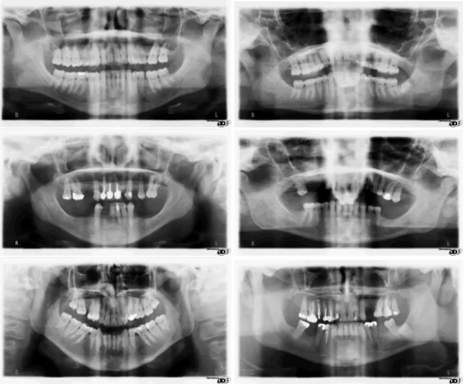
There are a total of 1392 grayscale images in the data set, with varying types of dental structure, sizes of the mouth and number of teeth per image, as can be seen in figure 3.2. The gray levels of each image were stretched to the [0, 255] scale, although both normalized and raw images will be soon available for download in the site of our research group Socia Lab.1

Another major point of interest of this data set is the set of maps that enable the manual detection and localization of dental cavities - for the moment - and other diseases in a near future. This is achieved by corresponding a binary image to each dental X-ray image thereby showing the regions with dental cavities. This will turn

1_{Socia Lab - Soft Computing and Image Analysis Laboratory, http://socia-lab.di.ubi.pt/}

(40)

24 CHAPTER 3. DATA-SET IMAGES

Figure 3.1: Picture of the Orthoralix 9200 DDE X-ray camera.

the data set into a preferable tool in the evaluation of method to perform automatic detection and localization of the respective diseases. Also, we believe that this set of images is useful to evaluate the current teeth segmentation methods as shown in 2.2.3.

3.2.1 Morphologic Properties

When compared with other types of stomatology images, radiographic images are highly challenging, due to several reasons that increase their heterogeneity:

1. Different levels of noise, due to the moving imaging device that captures a global perspective of the patient’s mouth.

2. Low contrast, either global or on local regions of the images, the topology and morphologic properties are very complex.

(41)

3.3. IMAGES STATISTICS 25

Properties Description Power Supply 115-250 VAC pm 10%

Frequency 50/60 Hz pm 2 Hz Maximum Line 10A at 250V,

Power Rating 20A at 115V

Anode Voltage 60-84 kV, in 2kV steps

Anode Current 3-15mA, in 1mA steps

Exposure Time 12s for standard pan,

0.16-2.5 s for Cephalometric

Duty Cycle 1:20 at full power operation

Focal Spot 0.5 mm, IEC 336 (1993)

Vertical Reach 39" to 71" (100 to 180 cm)

from floor to occlusal plane

Weight 410lbs (115 kg),

467lbs (212 kg) with Ceph arm

Active Area 147x6m (Standard Pan),

CCD Sensor 220x6m (Ceph)

Image Size 1536x2725 pixels (Standard Pan),

2304x2529pixels (Ceph-Maximum)

Table 3.1:Properties of the Orthoralix 9200 imaging device.

4. The noise originated by the spinal-column that covers the frontal teeth in some images, as shown in figure 3.2.

3.3 Images Statistics

The statistical study of the input images, consists in the extraction of some statistical features that are important and relevant to our work for our images data-set. With this study we can assume that some rules in the future steps of our method, and in some cases this type of empirical data could reveal themselves to be very important to some steps in our work.

(42)

Figure 3.2:Examples of images of the Dental X-ray data set.

3.3.1 Number of Teeth per Image

We considered that images contains all teeth in two different circumstances:

1. When the images include only the first and second molar, superior or inferior and left or right along with all other teeth.

2. When the images contain all three molars superior or inferior and left or right in addition to all other teeth.

In order to more effectively use the images we named them according to their charac-teristics. With this arrangement we classify the images based on the number of teeth and in the existence of dental cavities. The naming takes the form It1_t2_t3.tiff, where t1 corresponds to the image number, t2 represents the quantity of teeth per

(43)

3.3. IMAGES STATISTICS 27

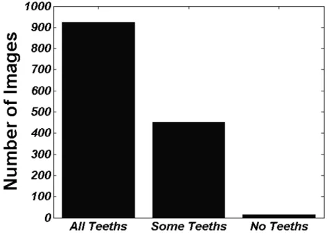
mouth (0 refers to no teeth, 1 to some teeth and 2 to all teeth) and t3 denominates the presence of dental cavities in the image (0 corresponds to no dental cavities and 1 to the presence of dental cavities). As an example, the name I1200_2_0.tiff corresponds to the image with id equal to 1200, which has all teeth and no dental cavities. In figure 3.3 is shown the count of the images data-set that fulfill the requirement of having all, some or none teeth.

Figure 3.3: Number of images concerning the quantity of teeth per mouth.

3.3.2 Average Size

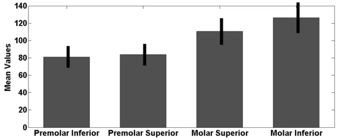
An adult individual has 32 teeth in is permanent teeth, the teeth are divided in two jaws, the upper a lower jaw, each one is constitute by 16 teeth. The composition of the mouth, concerning the teeth is on the left side constitute by three molars and two pre-molars, the front side contains four incisors two canine and finally the right side has three molars and two pre-molars. As reported in the beginning of this chapter, the data set contains many different dentition shapes and number of teeth per images. In figure 3.4 is given the interval for the average size of the teeth in 1000 sample size, with a 95% certainty. Note that for this study we only took into account the molars and pre molars, because they are in most cases the teeth

(44)

Figure 3.4: Average sizes and corresponding confidence intervals, regarding the type of teeth.

that missing in our input images. Based on our human nature, that missing teeth neighbors occupy the vacancy left by the missing teeth. This phenomenon is more visible in pre molars and molars.

3.3.3 Data Summary

Our main purpose of this section is to present the most important statistical charac-teristics of our data-set of images, consisting of 1392 grayscale images. In the table 3.2 are the statistics of all our images.

Note that the values are average values corresponding to all images, i.e., the mean value of intensities represented in the table 3.2, corresponds to the average value of intensities of all images.

As we can observe the mean intensities of all images present in our data-set images is a low mean value, this means that generally the intensities of each image is tend to be darker. This is also corroborated by the median value presented in the table 3.2. The maximum and minimum values show that exists a variety presence of almost all values belonging to the grayscale possible values. Finally the entropy that proves the fact that our images containing a large amount of information in the image, corresponding to the variety of types and properties of each image. The value of the entropy tend to decrease as we decrease the neighbor window. This proves that in small windows the changes in our images are inferior when comparing with larger neighbor windows.

(45)

3.4. CONCLUSION 29

Statistic Data Values Minimum intensity value 0

Maximum intensity value 252.1335

Mean intensity value 135.0296

Mode 240.7918 Variance 5227.9080 Standard Deviation 72.2699 Median 138.7947 Entropy 7.7920 Entropy (3x3) 2.0551 Entropy (9x9) 3.2412 Entropy (15x15) 3.6786

Table 3.2:Statistic date retrieve of our images data-set.

3.4 Conclusion

In this chapter we present our images data-set that have been essential to the development of our research. We present some relevant properties of our data-set images, such as the size of the teeth, the accounting number of images depending on the number of teeth present per image. To emphasize the importance of some data, boot statistic and empirical, in this chapter that will be used further on our method stages. In the next chapter is presented the firsts steps of our method, which are the ROI definition and the jaws partition.

(46)

(47)

Chapter 4 ROI Definition and Jaws Partition

This chapter will begin by describing the first steps of our method. In the first stage is elaborated the analysis of the distances between the center of the image and the four corners of the mouth. This with the aim of creating an area of interest, our ROI, an area which would contain only the mouth with their teeth. If so the removal of nasal and chin bones. In a second stage and having the first area of interest defined, we start to separate the jaws. Firstly by extracting points between the Jaws and then connect those points by the polynomial least squares fitting [63], which corresponds to derivation of the least squares fitting [38][62][17].

4.1 ROI Definition

The earliest stage is based in the statistical analysis of the sizes and positions of each component in each image, in order to define an initial region of interest. This eliminates non-useful information originated by the nasal and chin bones. Our purpose is to crop a region that contains the entire mouth and eliminate the maximum amount of noise possible. For each data set image we measured four distances (R1, R2, R3, R4), starting from the image center (xc, yc)=(w/2 = 1408, h/2 =

770), as shown in figure 4.1.

Having these values of all the data set images, we obtained the four histograms as illustrated in figure 4.2. Here, the line series correspond to the approximated normal distribution obtained by a line fitting procedure, defined by the (µ, σ) parameters.

Based on this distribution we can approximate the minimum value for each Ri

(48)

32 CHAPTER 4. ROI DEFINITION AND JAWS PARTITION

Figure 4.1: Four lengths extracted of our images data-set.

Figure 4.2: Histogram of the Rivalues.

thereby appropriately cropping the images with a 95% certainty. Furthermore, a defined margin guarantees that slightly different images will be appropriately cropped, even if a small increment of non-useful regions is included. The values obtained were R1 ≈ 897.77, R2 ≈ 863.36, R3 ≈ 406.31, and R4 ≈ 471.27. Figure 4.3

(49)

4.2. JAWS PARTITION 33

illustrate the final results of this stage.

Figure 4.3:Some results for the ROI definition.

As shown, the images contain only the mouth with their teeth. The fact that we choose to cut with a confidence level of 95% leads to the images that emerge out of that range will have areas of teeth cut, which would originate a non detection of dental caries in the corresponding teeth. Furthermore the images are within this range can have over presence of noise, because of the wide variety of size and structure of the mouth becomes more complicated to define the ideal size for each image.

4.2 Jaws Partition

In this stage we separate the upper and the lower jaws, which is done by applying a polynomial fitting process to a set of primitive pixels located between jaws. This set of pixels is based on the horizontal projection, v(u), of the images, given by 4.1, where I(x, i) denotes the intensity value at line x and column i.

v(u)=

w

X

i=0

(50)

The initial point is defined at the right extreme of the image and at the line that has the minimum v(u) value, given by 4.2, where w is the image width and shown in figure 4.4.

p0(x0, w − 1) = arg min

x (v(u)) (4.2)

Figure 4.4: Horizontal Projection of the intensities, for our starting point.

The remaining set of points pi are regularly spaced, starting from p0 : pi(xi, (w −

1) − W/21), where xiis obtained similarly to x0. To avoid too high vertical distances

between consecutive pi, we added the following constraints 4.3.

pi(xi, yi)=       

pi(xi+1+ T, yi), | pi(xi, yi) − pi+1(xi+1, yi+1) |> T

pi(xi, yi), otherwise

(4.3)

Empirically T is the threshold defined by us to avoid the high vertical distances, with the value of T= 20. We observed that this step plays a major role in dealing with missing teeth. This method to the extraction of the initial point is based on several proposals to perform the separation of jaws ([53][23][25]). Having the set of pi(xi, yi)

primitive points, the division of the jaws is given by the 10th _{order polynomial,}

given by 4.4, obtained by the polynomial least squares fitting algorithm, based on the Vandermond matrix [65]. This technique is able to achieve impressive accuracy on the data set images, as illustrated in figure 4.5 and summarized in table 7.1.

(51)

4.3. CONCLUSION 35

Figure 4.5:Results of the polynomial least squares fitting.

The process defined by us, to perform the jaws partition, is dependent on the size of the missing teeth present in the input image. If the teeth are missing and at the same time neighbors makes our method vulnerable to error, because the points extracted by us will tend to follow the darker areas of the image, and sometimes the areas in which missing teeth are darker when comparing to the gap between the jaws, after an considerable missing teeth area our method may be in some occasions capable to overcome the presence of a tooth, as shown in the figure 4.6.

A solution that can be implemented to improve this situation would be to divide the image into smaller stripes, when we are extracting the points, which in turn could make the method more sensitive to small changes of intensity in the image, making it even more difficult to separate the jaws.

4.3 Conclusion

In this chapter we present the first stage of our method, which consisted in defining a first area of interest, our ROI which with this step has been possible to eliminate much of the noise present in our input images. The second step was the jaws partition, by the extraction of 21 points between the jaws and the connection of this same points through the polynomial least squares fitting process, we have been able to separate the jaws for our data-set training images with a large percentage

(52)

Figure 4.6: Results of the polynomial least squares fitting in images with accentuated missing teeth area.

of success. In the next chapter is staging the next step of our method, the teeth gap valley detection. This step is divide in two methods, the first one is our primary version of the teeth gap valleys detection, which culminates with a acceptable article submission in the II Eccomas Thematic Conference on Computational Vision and Medical Image Processing (VIPImage’09). The second is our better improvement of the first version, through the use of the Active Contours Algorithm.

(53)

Chapter 5 Teeth Gap Valley Detection

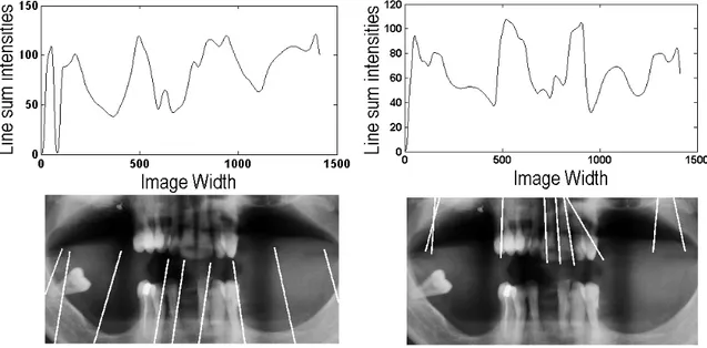
The next step in our method it is in the detection of the teeth gap valley where the aim is to get a zone containing only one tooth. The perfect output is when the output as many pictures then teeth in the image. To perform the detection of teeth gap valleys and based on the output generated by the polynomial obtained in the jaws partition. Next, we draw perpendicular lines to all points belonging to the polynomial. For each point it will be selected the line which the sum of intensities of the pixels belonging to the line is minimal. Finally the points are selected where the intensity is minimal, as can be seen in the figure 5.1. What we developed at this point as resulted in an article submitted to VIPImage’09.

5.1 Line Sum Intensities - Method 1

Having both jaws divided, our next goal was to localize the regions corresponding to each teeth, which is based on the detection of the gap valleys between them, because we are in presence of a darker zone, therefore the intensities between them is substantial inferior when compared with the teeth intensities. This rule is not applicable when referring to teeth overlap, in this case we have the opposite effect, an increase of intensity. This stage can itself be divided into three sub-stages:

1. For each pixel x between 0 and w − 1, where w is the image width, we obtain the equation of the perpendicular line to r(x) at the point (x, r(x)). Then, the average intensity a of the pixels that fall in that line is obtained. Due to the image properties, the shape of the teeth and the shape of the polynomial, we

Caries detection in panoramic dental x-ray images

João Paulo Ribeiro de Oliveira

Caries Detection in Panoramic Dental

X-ray Images

Universidade da Beira Interior

Departamento de Informática

João Paulo Ribeiro de Oliveira

Caries Detection in Panoramic Dental

X-ray Images

Acknowledgements

Contents

List of Figures

List of Tables

Acronym

Chapter 1

Introduction

1.1

Main Goal

1.2

Motivation

1.3

Computer Vision

1.4

Block Diagram

1.5

Organization

Chapter 2

State of the Art

2.1

Dental X-ray

2.1.1

X-ray

2.1.2

Stomatologic

2.1.3

Main Applications

2.2

Applications of Dental X-ray in Computer Science

2.2.1

Clinical Environments

2.2.2

Biometrics

2.2.3

Teeth Segmentation

2.2.4

Active Contours

2.3

Conclusion

Chapter 3

Data-Set Images

3.1

Dental X-ray camera

3.2

Properties

3.2.1

Morphologic Properties

3.3

Images Statistics

3.3.1

Number of Teeth per Image

3.3.2

Average Size

3.3.3

Data Summary

3.4

Conclusion

Chapter 4

ROI Definition and Jaws Partition

4.1

ROI Definition

4.2

Jaws Partition

4.3

Conclusion

Chapter 5

Teeth Gap Valley Detection

5.1

Line Sum Intensities - Method 1