Data Fusion in Internet of Things

(1)

Faculdade de Engenharia

Data Fusion in Internet of Things

Versão Final Após Defesa

Tiago Mendes

Dissertação para obtenção do grau de mestre

<Engenharia Informática>

2

o

_{Ciclo de estudos}

Coordinator: Prof. Doutor Nuno Pombo

Co-Coordinator: Prof. Doutor Nuno M. Garcia

Co-Coordinator: Prof. Sari Merilampi

(2)

(3)

Acknowledgements

In the end of the writing of my dissertation i have the following acknowledgements to do: in the first place i have to thank to my family, more specifically my parents and my uncle, and also my closest friends who always been there for me and helped me in whatever i needed. I also want to thank to my master’s degree colleagues Sérgio Silva and Miguel Rodrigues for all the support they provided. Finally i want to thank to my dissertation coordinators Professor Nuno Pombo and Professor Nuno M. Garcia from Universidade da Beira Interior and Professor Sari Merilampi from Satakunta University of Applied Sciences in Finland because they always provided valuable help, support and insight.

(4)

(5)

Summary

Internet of Things (IoT) brings the real physical world, virtual cyber world and digital world together. A myriad of sensors, such as mobile terminals, cameras, microchips, wearables and even the Internet, play an important role in IoT. These sensors collect, generate, and preserve a diversity of data with different representations, scales, and densities from various “things”, which offers IoT the ability to measure, infer and understand environments. Integrating things and data opens opportunities for knowledge discovery, and further makes it possible to provide advanced and intelligent services. Thus, data fusion is an essential and integral part of IoT, because integrates multiple data and knowledge into a consistent, accurate and useful representation, in which the data are fused to high-quality information to provide a reliable decision support. The base idea for this research is to create a computerized model with capability to fuse data from different sources in order to produce a reliable and accurate information. In addition, a practical system should be developed including the decision making on the adoption of sensors, data handling, metrics and outcomes produced by the system.

(6)

(7)

Abstract

This dissertation reviews Internet of Things concepts and implementations, state-of-the-art tech-nology with practical examples, as well as data fusion methods applied in different problems. The purpose of this study is to review different data fusion methods and develop a system to provide recognition of human activity that can be applied in day care homes and in hospitals to monitor patients.

The system’s objective is to study human activity recognition based on the data recovered by sen-sors like accelerometers and gyroscopes. In order to transform this data to useful information and practical results to monitoring patients with accuracy and high performance, two different neural networks were implemented.

To conclude, the results from the two different neural networks are compared to each other and compared with systems from other authors. It is hoped this study will inform other authors and developers about the performance of neural networks when managing human activity recognition systems.

Keywords

Internet of Things, Smart Home, Data Fusion, Deep Learning, Health-care, Human Activity Recog-nition, Neural Networks.

(8)

(9)

List of Figures

1.1 Convolutional Neural Network Basic Architecture . . . 2

1.2 Recurrent Neural Network Basic Architecture . . . 2

2.1 Decentralized architecture. Source: https://www.hindawi.com/journals/tswj/2013/704504/ 6 2.2 Distributed architecture. Source: https://www.hindawi.com/journals/tswj/2013/704504/ 6 2.3 Centralized architecture. Source: https://www.hindawi.com/journals/tswj/2013/704504/ 6 2.4 Smart home environment. Source: https://www.accenture.com/ae-en/insight-smart-home-smart-strategy . . . 8

2.5 Weka Smart Fridge. Source: https://internetofbusiness.com/iot-smart-fridge-vaccine-care/ . . . 10

2.6 HNC Telemedicine Platform. Source: https://healthnetconnect.com/offerings/telemedicine/ 11 2.7 KNN Classification. Source: https://www.analyticsvidhya.com/blog/2018/03/introduction-k-neighbours-algorithm-clustering/ . . . 13

2.8 Naive Bayes Example. Source: http://www.statsoft.com/textbook/naive-bayes-classifier . . . 14

2.9 Naive Bayes Example with classification. Source: http://www.statsoft.com/textbook/naive-bayes-classifier . . . 14

2.10 Support Vector Machine Example. Source: https://www.analyticsvidhya.com/blog/2017/09/understaing-support-vector-machine-example-code/ . . . 16

2.11 Artificial Neural Network. Source: https://www.digitaltrends.com/cool-tech/what-is-an-artificial-neural-network/ . . . 17

2.12 Convolutional Neural Network. Source: https://www.mdpi.com/2078-2489/7/4/61 18 2.13 Recurrent Neural Network. Source: https://colah.github.io/posts/2015-08-Understanding-LSTMs/ . . . 19

2.14 Long Short Term Memory Diagram . . . 20

3.1 Properties of the accelerometer sensor. . . 24

3.2 properties of the gyroscope sensor. . . 24

3.3 Example of measurements from the accelerometer sensor. . . 25

3.4 Example of measurements from the gyroscope sensor. . . 25

3.5 Example of records from the data set . . . 26

3.6 Sigmoid Activation Function . . . 28

3.7 Tanh Activation Function . . . 28

3.8 ReLu Activation Function . . . 29

3.9 Convolutional Neural Network System Flow Chart . . . 30

3.10 Recurrent Neural Network System Flow Chart . . . 32

4.1 Blueprint of MeWet smart home, with sensors. . . 34

4.2 Sensor names in Thingworx platform. . . 34

4.3 Data Split into train and test set. . . 35

4.4 System definitions. . . 36

4.5 Convolutional Neural Network Architecture . . . 36

4.6 Long Short Term Memory Architecture . . . 37

(12)

5.1 CNN matrix chart. . . 42 5.2 Chart of predicted and true values, being yellow the highest and purple the lowest. 43 5.3 CNN vs LSTM accuracy comparison with the same configurations. . . 45 5.4 CNN vs LSTM accuracy comparison with the most iterations. . . 46 5.5 Comparison of this system(CNN and LSTM) with other systems. . . 48

(13)

List of Tables

5.1 CNN Confusion Matrix. . . 41 5.2 RNN + LSTM Confusion Matrix . . . 43 5.3 RNN + LSTM different test accuracy for the different activities. . . 44

(14)

(15)

Lista de Acrónimos

UBI Universidade da Beira Interior IoT Internet of Things

CNN Convolutional Neural Network RNN Recurrent Neural Network LSTM Long Short Term Memory

(16)

(17)

Chapter 1

Introduction

The focus of this study is to improve people’s quality of life through data gathered by sensors installed in a smart home, monitoring all health related aspects as well as recognize activities in order to prevent unfortunate events. This first chapter will introduce the reader in this technological environment as well as explain the purpose of this research and its objectives.

1.1 Internet of Things

A simple explanation of the concept Internet of Things (IoT) is a system of interconnected devices that can transfer data to a platform. Any device that can connect to the internet and managed from a remote location is considered an IoT device. Other than laptops or smart phones, the variety of different devices is growing as the Internet of Things grows. We already have cars, smart houses, health monitoring devices and even smart parking systems [1] connected to the internet and consequently providing useful data. The data gathered by these devices can be analyzed and used to achieve an improvement of quality of life, health and well being.

1.2 Data Fusion

Raw data from each separate device may not be enough to make decisions or predictions, and sometimes can be misleading. In order to get a more efficient usage of this data, instead of getting individual measurements from a single sensor, we can combine data from multiple sensors with a process called data fusion. A well-known definition of data fusion provided by Hall and Llinas [2] is: “data fusion techniques combine data from multiple sensors and related information from associated databases to achieve improved accuracy and more specific inferences than could be achieved by the use of a single sensor alone.” To summarize, we can define data fusion as the process of merging multiple sources to get more relevant and higher quality information

1.3 Data Fusion Techniques

There are some data fusion techniques that were created to provide a meaningful representation of the sensor outputs. To classify those techniques, Durrant-Whyte [3] provided this criteria: - Complementary: Combining pieces of a large picture together. Data gathered from different type of sensors in the same environment may be used to obtain accurate information. .

- Redundant: Two or more sensors providing data of the same target may increase accuracy and reliability.

- Cooperative: Putting together data from the original source and a more complex one, for example, audio and video.

A full review of data fusion techniques is available in Castanedo’s article [4] as well as its classifica-tion and the state-of-the-art techniques and methods are described in more detail on the following chapter.

(18)

Even with sophisticated techniques, there are some problems to solve, or some obstacles, for ex-ample, some of the readings provided by a sensor could be noise or not viable for analysis.

1.4 Methods

The method proposed to develop this system is an artificial neural network, more specifically, a Convolutional Neural Network (CNN) and a Recurrent Neural Network(RNN) with Long Short Term Memory(LSTM) extension. The CNN architecture is shown on figure 1.1 and the RNN architecture is shown on figure 1.2.

Figure 1.1: Convolutional Neural Network Basic Architecture

Figure 1.2: Recurrent Neural Network Basic Architecture

These methods will be explained extensively and a justification on why they were chosen is also provided.

1.5 Guidelines

At this point, the reader is prepared to understand this technological field of study and is aware of the context. In order to explain and analyze these technologies and processes, it was made an extensive review of articles in this field of study, as well as getting information from companies like

(19)

SICK Sensor Intelligence and other health care IoT solutions. All the software tools used will all be described in the implementation chapter.

1.6 Motivation and Objectives

The focus of this work is to explore the field of Internet of Things with data fusion principles in the health care field as well as implementing a tool for analyze data from a smart home. This research has three main objectives:

- Present a full review of all the main data fusion methods and techniques;

- Develop a prototype software capable for human activity recognition through data fusion meth-ods and sensor data;

1.7 Thesis outline

This dissertation is divided in chapters, explaining and describing all methods and technologies implemented and why, as well as a review of the problem and the solution proposed. The first chapter takes the reader to the internet of things and data fusion environment by explaining a few concepts of these fields as well as pointing the objectives of this study and the problem that was proposed. The second chapter defines the state of the art data fusion by presenting its architecture, methods and algorithms, as well as the most recent and innovative technologies applied recurring data fusion’s methods. The third chapter states the type of sensors used, the type of data and the methods applied and an explanation on how the data flows through the system. The chapter number four reports the actual implementation of the system with all the technologies and methods used and why. The results of this work can be found in the fifth chapter which compares the outputs of two different approaches and also a comparison with work results of another authors. The final chapter is reserved for all the conclusions and what was accomplished during this work as well as future work.

(20)

(21)

Chapter 2

State of the Art

2.1 Data Fusion Techniques

2.1.1 Introduction to Data Fusion

Data fusion is known as the process of taking multiple sources of information and combine them together in order to get efficient and accurate information and improving the decision support system. Surrounding a problem with many analytical tools will maximize the information recovered from data. There are different types of data fusion: low, intermediate and high-level data fusion distinguishing geospatial types of data fusion from other types of data fusion. Another specific type of data fusion is called “sensor fusion” where data from multiple sensors is combined into one data-rich image or analysis. In the next section, it is described the architecture of this process.

2.1.2 Data Fusion Architecture

There are some data fusion techniques that were created to provide a meaningful representation of the sensor outputs. To classify those techniques, Durrant-Whyte [3] provided this criteria:

- Complementary: Combining pieces of a large picture together. Data gathered from different type of sensors in the same environment may be used to obtain a more complete information. .

- Redundant: Two or more sensors providing data of the same target may increase accuracy and reliability.

- Cooperative: Putting together data from the original source and a more complex one, for example, audio and video.

Data fusion can also be classified according to its architecture (Figures 2.1, 2.2 and 2.3). There are a few differences between distributed and decentralized architecture. The first one preprocesses the measurements to a vector of features which are fused after. The decentralized architecture fuses the data in each node and shared information instead of states. The centralized architecture has a higher computational and communication cost due to the fact that the distributed nodes conduct other tasks before performing data fusion.

(22)

Figure 2.1: Decentralized architecture. Source: https://www.hindawi.com/journals/tswj/2013/704504/

Figure 2.2: Distributed architecture. Source: https://www.hindawi.com/journals/tswj/2013/704504/

Figure 2.3: Centralized architecture. Source: https://www.hindawi.com/journals/tswj/2013/704504/

A full review of data fusion techniques is available in Castanedo’s article [4] as well as its classifi-cation.

(23)

The fast changing technology world never ceases to amaze us with new state of the art technologies, and the Internet of Things is not an exception. In the Health-care field, the IoT industry is growing exponentially due to the steadily aging population, the high demand of doctors and nurses [5] , and the rise of chronic illnesses. Following Instituto Nacional de Estatística (INE), in Portugal, the population with the age of 80 or more has doubled in the last two decades which consequently increases the amount of monitoring and care services required.

It is humanly impossible for someone to take care of an old person or a sick child 24/7, so the IoT and consequently data fusion comes to aid, or at least ease the pressure of health care and health monitoring.

(24)

2.2 Smart Home Environment

A smart home environment can be defined as a small physical world, consisting of different devices, including sensors, actuators, displays and computational elements interacting and exchanging in-formation with users to provide them with automated, customized, and secured services. These types of environments are designed to make life better and secure through information processing. The need for automated and digital environments is increasing to provide better facilities and improve the quality of life. Not only smart homes are evolving technologically but also hospitals and day care centers are increasingly equipped with sensors and computational elements to become more efficient.

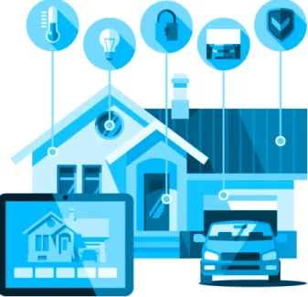
In a typical smart home environment, Internet of Things formed by the integration of all types of devices that are ready to gather all the data required so the smart home can work efficiently. Different sensors might be placed in different locations like kitchens, bathrooms, bedrooms, living rooms and even in garages like the example in figure 2.4.

Figure 2.4: Smart home environment. Source:

https://www.accenture.com/ae-en/insight-smart-home-smart-strategy

To better understand how a smart house works, in[6], the authors made a survey of the definition of smart homes to its current research status.They describe the smart home elements, research projects, smart home networks research status, smart home appliances and challenges. This paper provides a full review on smart home environments as well as its devices and networks.

(25)

2.2.1 Advantages and Disadvantages

One of the main advantages of smart homes is providing peace of mind to its inhabitants, allowing them to monitor their homes remotely, avoiding dangers such as a front door left unlocked or leaving dangerous devices left on like toasters or ovens.

Smart homes are also beneficial for the elderly, providing monitoring that can ensure them to remain at home comfortably and safely, rather than moving to a nursing home or requiring 24/7 home care.

Smart homes also helps its inhabitants to improve efficiency. Instead of leaving the lights on all day, a smart home system can learn behaviors and make sure that the lights are only on when needed. With home automation, energy, water and other resources are used more efficiently, which helps save both natural resources and money for the consumer.

However, smart home systems have struggled to become popular due to their technical nature and complexity. Some people have difficulty with technology or will give up on it with the first problem. Smart home manufacturers are working on reducing complexity and improving the user experience to make it enjoyable and beneficial for users of all types and technical levels.

For smart homes to be truly effective, devices must be universal regardless of who manufactured them and must use the same protocol. As it is a recent market, there is standard for smart homes yet.

Another major issue is smart home security. It is possible to someone who hacks a smart home system to turn off the alarms and unlock the doors, leaving a home defenseless. All the data acquired by the smart home devices is also vulnerable to anyone who has access to it. In addition to security, another issue is data privacy. While smart home devices manufacturers may collect consumer data to improve their products or offer new and improved services, some costumers do not completely trust on sharing their personal data.

(26)

2.3 State-of-the-art technology

Through wearable technology it is possible to early detect risk factors that may lead to a serious illness or even a chronic illness. There are a variety of sensors used to measure simple data like hearth rate, daily activity, human movement, insulin levels and so on, that are constantly being upgraded and innovated. The data gathered from those devices can be put through a series of data fusion techniques to be fully understandable and more trustworthy on the matter of decision support systems. However, these wearables should be practical, easy to use, and non-invasive, otherwise, they would be redundant [7].

Besides wearable sensors, there are state-of-the-art technology implemented to improve health care and health monitoring efficiency. The following sections indicate and describe some interesting examples as it would be impossible to point them all out because the world is full of different kinds of modern devices.

2.3.1 Weka Smart Fridge

Weka Smart Fridge from Weka Health Solutions is designed to improve vaccine management in order to get more people protected against diseases. This smart fridge includes a remote monitoring system to ensure the vaccines are stored at the proper temperature and it also manages how the vaccines are distributed. An example is shown on figure 2.5. Alan Lowenstein, COO of Weka Health Solutions says: “Clinicians in areas of Africa and other regions where power is unstable or inaccessible can use our Smart Fridge to store and dispense vaccines. And the Fridge is small enough that you can put it in a van. So if you can’t bring the people to the vaccine, you can bring the vaccine to the people.”

Figure 2.5: Weka Smart Fridge. Source: https://internetofbusiness.com/iot-smart-fridge-vaccine-care/

2.3.2 HNC Remote Patient Monitoring

Health Net Connect developed a remote patient monitoring system to support chronic diseases management. Patients remotely upload their data like real-time vitals, blood pressure, blood glu-cose, and weight. This data is encrypted and securely transferred using FIPS 140-2 encryption and transmitted to a platform where is reviewed by Health care professionals.An example of this platform is shown on figure 2.6.

(27)

Figure 2.6: HNC Telemedicine Platform. Source: https://healthnetconnect.com/offerings/telemedicine/

2.3.3 Deloitte Smart Helmet

Fall detection wearable technologies are developed not only for the elderly people but also for industries and workplaces. One good example of that is the Deloitte Smart Helmet. The Smart Helmet is an industrial-grade wearable device that facilitates safer productivity in heavy industries. It has a modular sensor suite that enables situational awareness for both the workers and the industrial operators. Combined with its range of connectivity features, this device allows workers and operators to identify early warning signs of impending danger within the surrounding area and communicate an action plan to mitigate the safety risks. Besides fall detection, this device also has other features like outdoor and indoor location tracking, mobile worker situational awareness, workplace safety and worker health monitoring. More information about this technology can be fount at https://cortex-design.com/work/deloitte/.

2.3.4 Angel 4

Angel4 by Sense4Care provides automatic fall detection due to a triaxial accelerometer and a specific algorithm.

The system consists of a small sensor which is placed at the waist with a belt and is connected to the telecare system, the health center or your mobile phone. Once a fall is recorded, a countdown is starting but can be interrupted by the user. If not interrupted, the system performs an emergency call and sends several SMS indicating the user situation and GPS location. More information about this technology can be found at https://www.sense4care.com/tienda/angel4-fall-detection/.

2.3.5 Intelligent Camera

A team of students in TU Delft university developed an intelligent camera designed for fall detection systems. This systems consists on a single wide angle camera mounted on the ceiling of a day care home. This gives a top view image of the environment resulting in a clear map of household objects without any occlusions. The main idea is to monitor the motion information of elderly and to model actions as a change of motion or poses in time that leads to a specific action.

All of the examples above depict the importance of IoT in helping and monitoring patients. A complete survey about the IoT role in health care and its architecture is provided by S. M. Riazul Islam, et al.[8].

(28)

2.4 State-of-the-art Methods

There are various ways to merge and fuse data through different methods and algorithms. In order to decide which method or methods to apply, they need to be surveyed to understand how they work and which one is better to each specific problem. This section is a survey of the main machine learning, deep learning and data fusion methods.

2.4.1 K-Means

The K-Means is a clustering algorithm using the number of clusters k and data sets as inputs. This algorithm begins with estimates for the K centroids, which are randomly selected from the data set. After that, the algorithm iterates between two steps:

1. Data assignment:

Each centroid defines one of the clusters. In this phase, each data point is assigned to its nearest centroid, based on the squared Euclidean distance. More formally, if

ci (2.1)

is the collection of centroids in set C, then each data point x is assigned to a cluster based on

arg min

ci∈C

dist(ci, x)2 (2.2)

where dist( · ) is the standard Euclidean distance. Let the set of data point assignments for each ith cluster centroid be Si.

2. Centroid update:

In this step, the centroids are recalculated. This is done by assigning new values to all data points assigned to that centroid’s cluster.

ci= 1 |Si| X xi∈Sixi (2.3)

The algorithm iterates between steps one and two until a stopping criteria is met (i.e., the data points cannot change clusters, the sum of the distances is minimized, or some maximum number of iterations is reached).

This algorithm is guaranteed to converge to a result. The result may be a local optimum (i.e. not necessarily the best possible outcome), meaning that assessing more than one run of the algorithm with randomized starting centroids may give a better outcome.

k-means can typically be applied to data that has a smaller number of dimensions, numeric, and continuous. For example, a scenario in which there is a need to make groups of similar things from a randomly distributed collection of things. An example of an implementation of this algorithm to predict students academic performance can be found in [9].

(29)

2.4.2 K-Nearest Neighbors

This algorithm specifies a positive integer k, along with a new sample. Then, a selecting process occurs to pick up the k entries in the database which are closest to the new sample. The most common classification of these entries is found and given to the new sample. The KNN stores the entire training data set and is used as its representation. Although the KNN does not learn any model, it makes predictions by calculating the similarity between an input sample and each training instance.

Figure 2.7: KNN Classification. Source:

https://www.analyticsvidhya.com/blog/2018/03/introduction-k-neighbours-algorithm-clustering/

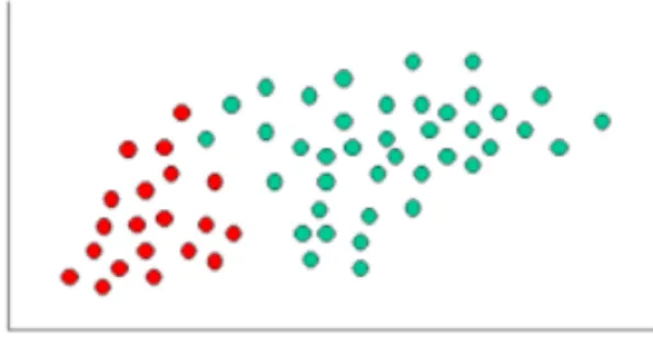
In figure 2.7, the test sample (green circle) should be classified either to the first class of blue squares or to the second class of red triangles. If k = 3 (solid line circle) it is assigned to the second class because there are 2 triangles and only 1 square inside the inner circle. If k = 5 (dashed line circle) it is assigned to the first class (3 squares vs. 2 triangles inside the outer circle).

(30)

2.4.3 Naive Bayes

The Naive Bayes method is a probabilistic classifier recurring to features and classes. To determine the probability of the features occurring in each class, in order to return the most likely class, this method uses the Bayes rule:

P (A | B) = P (B | A) P (A) P (B) (2.4)

To demonstrate the concept of Naive Bayes Classification, an example is displayed in figures 2.8 and 2.9. As indicated, the objects can be classified as either GREEN or RED. The task is to classify new cases as they arrive, i.e., decide to which class label they belong, based on the currently exiting objects.

Figure 2.8: Naive Bayes Example. Source: http://www.statsoft.com/textbook/naive-bayes-classifier

Since there are twice as many GREEN objects as RED, it is reasonable to believe that a new case (which hasn’t been observed yet) is twice as likely to be GREEN rather than RED. In the Bayesian analysis, this is known as the prior probability. Prior probabilities are based on previous experience, in this case the percentage of GREEN and RED objects, and often used to predict outcomes before they actually happen.

Since there is a total of 60 objects, 40 of which are GREEN and 20 RED, the prior probabilities for class membership are depicted in figure 2.9:

Figure 2.9: Naive Bayes Example with classification. Source: http://www.statsoft.com/textbook/naive-bayes-classifier

Having formulated the prior probability, the next step is to classify a new object (WHITE circle). Since the objects are well clustered, it is reasonable to assume that the more GREEN (or RED) objects in the vicinity of X, the more likely that the new cases have that particular color. To measure this likelihood, a circle around X is drawn which involves a number of points irrespective of their class labels. Then the number of points in the circle belonging to each class labels are

(31)

calculated. From this it is calculated the likelihood.

Although the prior probabilities indicate that X may belong to GREEN (given that there are twice as many GREEN compared to RED) the likelihood indicates otherwise; that the class of X is RED (given that there are more RED objects in the vicinity of X than GREEN). In the Bayesian analysis, the final classification is produced by combining both sources of information, i.e., the prior and the likelihood, to form a posterior probability using the so-called Bayes’ rule (named after Rev. Thomas Bayes 1702-1761).

Finally, X is classified as RED since its class membership achieves the largest posterior probability.

The Naive Bayes Classifier is used for making predictions in real time due to its fast and dynamic learning properties. It is also known for it multi class prediction feature, i.e., it can predict the probability of multiple classes of a determined variable. This classifier is mostly used in text classification, it has higher success rate when compared to other methods because of the better results in multi class problems. An example of this algorithm implemented for educational classification can be found at [11].

(32)

2.4.4 Support Vector Machine

Support Vector Machine (SVM) is a supervised machine learning algorithm which can be used for both classification and regression problems. In this algorithm, each data item is plotted as a point in n-dimensional space (where n is the number of features) with the value of each feature being the value of a particular coordinate. Then, the classification is performed by finding the hyper-plane that distinguish the two classes. This algorithm does some extremely complex data transformations, then figures out how to separate data based on the labels or outputs previously defined.

Figure 2.10: Support Vector Machine Example. Source:

https://www.analyticsvidhya.com/blog/2017/09/understaing-support-vector-machine-example-code/

Support Vectors are simply the co-ordinates of individual observation. Support Vector Machine is a frontier which best segregates the two classes (hyper-plane/ line) like the example in figure 2.10. The distance between the hyperplane and the nearest data point from either set is known as the margin. The objective is to choose a hyperplane with the greatest possible margin between the hyperplane and any point within the training set, giving a greater chance of new data being classified correctly.

The SVM algorithm is accurate and works better on smaller data sets and the efficiency can be increased using a subset of training points. This method is best used on text classification, image recognition and handwritten digit recognition. An example of this algorithm implementation on data classification can be found in [12]

(33)

2.4.5 Artificial Neural Network

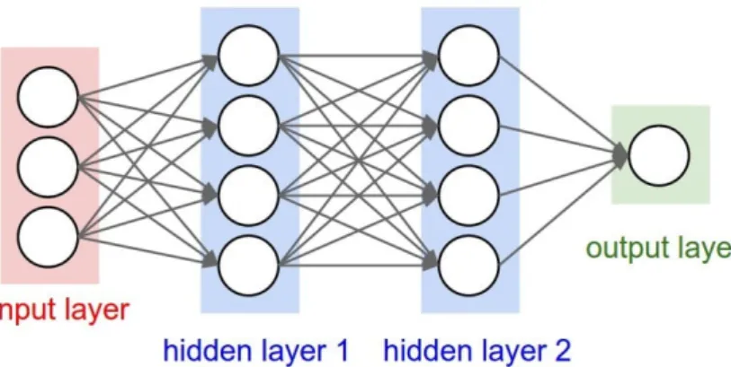
An artificial neural network (ANN) is one of the main methods used in machine learning. It is a system inspired in the human brain which intends to replicate the way that the humans learn. Neural networks consist of input and output layers, as well as (in most cases) a hidden layer consisting of units that transform the input into something that the output layer can use. The ANN is an efficient method for finding patterns which are far too complex for a human to extract and teach the machine to recognize by its own.

Figure 2.11: Artificial Neural Network. Source:

https://www.digitaltrends.com/cool-tech/what-is-an-artificial-neural-network/

In figure 2.11, the data set is input in the first layer, then each layer extract a different set of high-level features. For example, in image recognition, the first layer recognizes the pixels’ brightness, the next layer recognizes textures and shapes and the next one the edges of the image and so on. The output is labeled and then occurs the back propagation effect to correct any mistakes that might have been made. After some iterations, the network is self capable of executing any classification tasks without the help of a human.

The neural networks are capable identifying patterns in data. The most specific actions are clas-sification (classifying data sets into predefined classes), clustering (classifying data into different undefined categories), and prediction (using past events to guess future ones, like the stock mar-ket). The ANN can be found in cars that can drive autonomously on the roads, in the creation of realistic CGI faces, in machine translation, fraud detection, used on smart homes and health care services like human activity recognition.

Of course there are various types of neural networks, each one specifically designed for a specific use. The most simple neural networks have information travelling only from input to output and are called feed forward neural network.

A more widely used type of network is the recurrent neural network, in which data flows in multiple directions. These neural networks have greater learning abilities and are implemented for more complex tasks such as human activity recognition or language recognition.

There are also convolutional neural networks, Boltzmann machine networks, Hopfield networks, and many others. The process of choosing the more appropriate neural network for the problem at hand depends on the kind of data available for training and the specific application. It is also possible to use more than one network when facing a more challenging problem.

(34)

2.4.5.1 Convolutional Neural Network

A Convolutional Neural Network (CNN) is a category of Neural Networks that have proven very effective in areas such as image recognition. CNN’s have been successful in identifying faces, ob-jects and traffic signs and powering vision in robots and self driving cars.

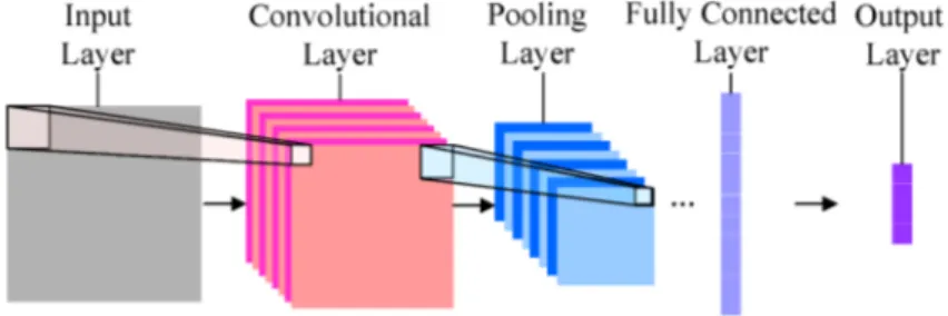
CNN’s derive their name from the “convolution” operator. The primary purpose of convolution in case of a CNN is to extract features from the input. For example, when the input is an image, convolution preserves the spatial relationship between pixels by learning image features using small squares of input data. CNN architecture is composed by three main types of layers: Convolutional Layer, Pooling Layer, and Fully-Connected Layer. These layers are shown in figure 2.12.

Figure 2.12: Convolutional Neural Network. Source: https://www.mdpi.com/2078-2489/7/4/61

The first part of a convolutional layer is called the kernel or filter which is responsible for capturing the low-level features such as edges, color, gradient orientation, etc, when the input data is an image. With added layers, the architecture adapts to the high-level features as well, resulting on a network which has a better understanding of images in the dataset.

Similar to the convolutional layer, the pooling layer is responsible for reducing the spatial size of the convoluted feature. This is to decrease the computational power required to process the data through dimensionality reduction. Furthermore, it is useful for extracting dominant features which are rotational and positional invariant, thus maintaining the process of effectively training of the model.

Fully connected layers connect every neuron in one layer to every neuron in another layer. It is in principle the same as the traditional multi-layer perceptron neural network (MLP). The flattened matrix goes through a fully connected layer to classify the images. After a set amount of convolutions and pooling, the final output is put through a fully connected layer, which is a conventional feed forward neural network to output a result. An example of this neural network implementation on real-time object detection can be found in [13]. Although this neural network is most used in image recognition, it is also used in time series problems.

(35)

2.4.5.2 Recurrent Neural Network

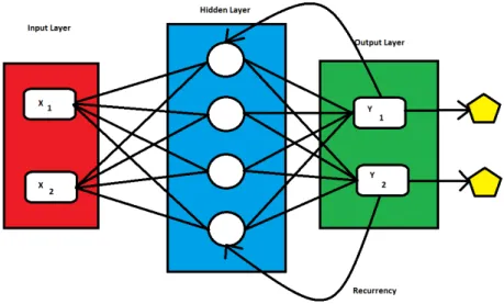
A recurrent neural network (RNN) is a type of artificial neural network (ANN) that has data flows on multiple directions and they have the ability to build on earlier types of networks with fixed-size input vectors and output vectors. This type of network have a memory which captures information of what was calculated so far. Unlike other neural networks, the RNN’s inputs are related to each other. The way that RNN works begins with a simple input from a dataset which is computed using randomly initialized variables to produce a predicted result. Then, that result is compared to the expected value and an error value is obtained. Using that error value through the same path will adjust the variables. This procedure is called the back propagation algorithm. These steps are repeated until the variables are well-defined, a status which is decided by the person who is operating the RNN. The predictions are made by applying these variables to untrained inputs. An example is shown on figure 2.13.

Figure 2.13: Recurrent Neural Network. Source: https://colah.github.io/posts/2015-08-Understanding-LSTMs/

The RNN is best applied in image caption, time series anomaly detection, stock market prediction, speech recognition and other complex problems. An example of RNN implementation for text classification with multi-task learning can be found in [14].

(36)

2.4.5.3 Long Short Term Memory Network (LSTM)

For solving a time series problem, any RNN would do just fine. However, there are cases that need a long-term context and sometimes a normal RNN is not able to reach it. Long Short Term Memory networks (LSTM) are a special kind of RNN, capable of learning long-term de-pendencies. They were introduced by Hochreiter and Schmidhuber in 1997, and were upgraded by various researchers in following work. More information about LSTM history can be found at https://www.analyticsindiamag.com/meet-juergen-schmidhuber-the-father-of-lstm-an-outsider-in-the-world-of-deep-learning/.

They work very well on a large variety of problems, and are now widely used.

LSTMs are designed to avoid the long-term dependency problem. They can remember information for long periods of time.

All RNN’s repeat modules of a neural network. In standard RNNs, this repeating module will have a structure called the tanh layer. Instead of having a single neural network layer, LSTM has four interacting layers.

σ σ σ X

₊

X t

h t

tanh X X tanh

LSTM

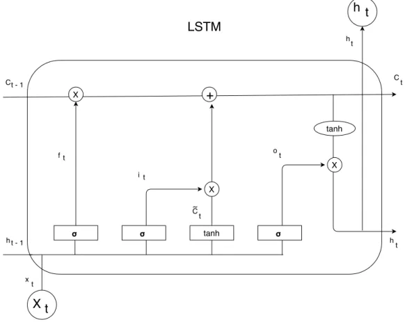
h t - 1 f t x t i t Ct - 1 C t ~ h t C t h t t o

Figure 2.14: Long Short Term Memory Diagram

Following the diagram in figure 2.14, the horizontal line running through the top of the diagram is called the cell state which flows information easily unchanged. The LSTM does have the ability to remove or add information to the cell state, regulated by structures called gates. Gates are a way to optionally let information through. They are composed out of a sigmoid neural net layer and a multiplication operation.

The sigmoid layer output are numbers between zero and one depending on how much of each component should be let through. This looks at ht−1 and xt, and outputs a number between 0

(37)

the biases of the respective gates.

ft= σ (Wf· [ht−1, xt] + bf) (2.5)

Next, a decision is made regarding what new information needs to be stored in the cell state. A sigmoid layer decides which values to update and a tanh layer creates a vector of new values that can be added to the cell state, ˜Ct. Combining these two creates an update to the state.

it= σ (Wi· [ht−1, xt] + bi) (2.6)

˜

Ct= tanh (WC· [ht−1, xt] + bC) (2.7)

The previous cell state Ct−1is now updated into the new cell state Ct. The decision above is taken,

and it is executed here by multiplying the previous cell state by ftand add it ˜Ct originating the

new values.

Ct= ft∗ Ct−1+ it∗ ˜Ct (2.8)

The final step is deciding the output which will be based on the cell state with some alterations. These alterations consist in running a sigmoid layer to decide what parts of the cell state is going to be output. After that, the cell state is put through a tanh layer with values between -1 and 1. Both of this outcomes are multiplied in order to get the desired output.

ot= σ (Wo· [ht−1, xt] + bo) (2.9)

ht= ot∗ tanh (Ct) (2.10)

The LSTM is most applied in robot control, time series prediction, speech recognition, rhythm learning, music composition, grammar learning handwriting recognition and human action recog-nition.

2.4.6 Conclusion

This chapter surveyed the main data fusion methods, explaining them and pointing out their uses and advantages and disadvantages.The LSTM extension is excellent at holding long term memories. The prediction of the nth sample in a sequence of test samples can be influenced by an input that was given many time steps before. The network can store or release memory on the go through the gating mechanism.

(38)

(39)

Chapter 3

Methods

3.1 System

The proposed system is based on using two sensors, an accelerometer and a gyroscope imbued in any modern smartphone to gather data from subjects in a smart house, in order to build an human activity recognition software. All the sensors, data gathered, and methods are explained in the following section.

3.2 System Properties

3.2.1 Introduction

The main objective of this project is to achieve results to help people monitoring their own lives, or the lives of their relatives in need, with the implementation of data fusion and Internet of Things in the health care field regarding the human activity recognition as its main field. This section describes various kinds of sensors applied on a smart home and others used specifically in this project, the data they provide and the best models suited for this problem and why. After stating this system’s properties, the structure with accurate data and code flow charts is explained.

3.2.2 Sensors

There are different kinds of sensors used in this system, however, not all of them provide the data needed to get the pretended results. In order to get the best outputs, the more efficient sensors for human activity recognition will be tested as well as smartphones with imbued accelerometers and gyroscopes.

The technical information about each sensor and their possible status can be consulted below:

- Sick scanner, a sensor from SICK Sensor Intelligence (on/off) – data in front of the bedroom door, from 3 different regions, SICK scanner type is TIM361;

- Kitchen water faucet: (on/off), signal from faucet is 12V-AC; - Apartment door (open/closed);

- Outdoor temperature, sensor type is Pro dual TEU PT1000 EAN 6419767005311; - Indoor temperature, sensor type is Pro dual TEHR PT1000 EAN 6419767005472;

- Smartphones (OnePlus X) with imbued accelerometers and gyroscope to measure human activity;

(40)

Figure 3.1: Properties of the accelerometer sensor.

Figure 3.2: properties of the gyroscope sensor.

3.2.3 Data

The type of gathered data is important to determine which methods are more efficient to compute it. Regarding this information, the data set needs to have its data preprocessed in order to improve accuracy and to best suit the model.

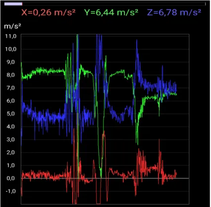
The ideal type of data is the data gathered from the accelerometers and gyroscopes since these are the most adequate available sensors to recognize human activity. The sensor signals (accelerome-ter and gyroscope) were preprocessed, getting data files named "gyroscope.csv" and "accelerome-ter.csv", respectively. Before the data is processed into an efficient data set, it can be visualized in charts, represented in figures 3.3 and 3.4:

(41)

Figure 3.3: Example of measurements from the accelerometer sensor.

Figure 3.4: Example of measurements from the gyroscope sensor.

The data is then sent to a computer, in this case it was sent via e-mail, and then processed into a data set. An example of this data set is shown on figure 3.5. Each record of data provides a tri-axial acceleration from the accelerometer (total acceleration) and the estimated body acceleration,

(42)

triaxial Angular velocity from the gyroscope, a vector with time and frequency domain variables and its activity label.

Some data was gathered from these sensors, but due to the lack of subjects and technology available, the data set was not ideal to obtain a high performance from this system in terms of number of samples. The rest of the data set was constructed from a data set available free at

https://archive.ics.uci.edu/ml/datasets/Smartphone+Dataset+for+Human+Activity+Recognition+(HAR)+in+Ambient+Assisted+Living+(AAL). It was only used a part of this data set due to its properties regarding triaxial acceleration and

angular velocity.

(43)

3.2.4 Data Model

The decision of which data model to implement is very important to the system because not only will test which approach is better to solve the problem proposed but also it will be indispensable to produce the best results possible and consequently the best possible system performance achievable from the obtained data.

Simple neural networks would be more efficient for this type of problem than any other method because they take a different approach to problem solving than that of conventional methods. Conventional methods use an algorithmic approach i.e. the method follows a set of instructions in order to solve a problem but as an advantage they also use less computing resources than neural networks. The neural networks process information in a similar way the human brain does. The network is composed of a large number of highly interconnected processing elements (neurons) working in parallel to solve a specific problem. In situations there are some relationships between inputs and outputs that are non- linear and complex. Neural networks have the ability to learn and model these non-linear and complex relationships and they are widely used in pattern recognition because of their ability to generalize and to respond to unexpected inputs.

After a review of the best machine learning, deep learning and data fusion methods, it was de-cided to pursue two different paths. The first is using a Convolutional Neural Network in order to process the data gathered by the sensors into information that could be useful in decision making systems or work with human activity recognition. The second is implementing a Recurrent Neural Network with Long Short Term Memory which extends the neural network memory and improves its performance.

The main difference between a Convolutional Neural Network (CNN) and a Recurrent Neural Network (RNN) is that CNN considers only the current input while RNN considers the current input and also the previously received inputs. RNN works on the principle of saving the output of a layer and feeding this back to the input in order to predict the output of the layer. This neural network uses activation functions that defines the output of a node given an input or set of inputs introducing non-linear properties to the network.

Recurrent networks, of which LSTM is one of the most successful, are generally useful when dealing with a time series and with sequential data. However, normal RNNs fail to understand the context behind an input and LSTM takes care of a long dependency problem that other RNNs have.

(44)

3.3 Methods

3.3.1 Activation Functions

Amongst all the activation function, the most popular are the Sigmoid, Tanh(Hyperbolic tangent) and ReLU (Rectified linear units).

The Sigmoid function takes a value as input and outputs another value between 0 and 1. It is non-linear and easy to work with when constructing a neural network model. The advantage of this function is that continuously differentiable over different values of z and has a fixed output range.

Sigmoid functions are used especially in binary classification models as part of the output layer to capture the probability ranging from 0 to 1 as shown on figure 3.6.

Figure 3.6: Sigmoid Activation Function

The Tanh function is a modified version of the sigmoid function. In Sigmoid the value of f(z) is bounded between 0 and 1 as shown on figure 3.7; however, in the case of Tanh the values are bounded between -1 and 1.

Having a wider range output, it is able to get values of different signs, which helps in establishing which scores to consider in the next layer and which to ignore.

Figure 3.7: Tanh Activation Function

The Rectified Linear Unit (ReLU) function is considered the most commonly used activation function in deep learning models. The function simply outputs the value of 0 if it receives any negative input, but for any positive value z, it returns that value back like a linear function. However, it should be noted that the ReLU function is still non-linear so it can have multiple layers of neurons.

(45)

The ReLU function has a derivative of 0 over half of its range which spans across all the negative numbers. For positive inputs, the derivative is 1 as shown in figure 3.8. It is computationally economical compared to Sigmoid and Tanh. ReLU has its own set of limitations and disadvantages like the dead neurons problem that if the units are not activated initially, then they are always in the off-state as zero gradients flow through them (Dead Neurons). However, the ReLu function is a better activation function than its other non-linear alternatives.

It is best used in between the input and output layers, more specifically within hidden layers.

Figure 3.8: ReLu Activation Function

In this system, the LSTM will use a sigmoid function due to its simplicity when working with neural networks.

3.3.2 System’s data flow

In this section it is explained how the two models are implemented and how the data flows from the loading of the data set to the final results with the help of flow charts.

3.3.2.1 CNN model

Following figure 3.9, in (1), a chunk of data is selected from the data set mentioned in this chapter and is loaded to the system. The labels for the different activities are also defined in this step, which are "Sitting", "Standing", "Walking", "Walking Downstairs", "Walking Upstairs" and "Laying", activities which were measured with the help of the accelerometer and gyroscope sensors.

After the data is loaded, the model separates data in two different sets in step (2), the train set which is the actual data set that is used to train the model and the test set which is only used after the model is fully trained and is used to evaluate the final model fit on the training data set. Before the model is built, step (3) is essential to configure the system properties, for example, the definition of the number of epochs or iterations, the number of neurons used and the batch size which means how many samples are trained each iteration. In (4), the data is loaded in the model and trained. The data flows through a series of layers. The convolutional layer is the first layer to extract features from an input. The pooling layer would reduce the number of parameters when the data sets are too large. The fully-connected layer combines all the features together to create a model.

The test set is then used to compare the results and the output is in the form of a confusion matrix with predicted and true values in step (5).

(46)

Once the confusion matrix is built the system produces a chart with these values in order to fully understand the results (6).

(47)

3.3.2.2 LSTM Model

Following figure 3.10, in (1), the data is loaded from the data set into the system. In step (2), that data is divided into a train and test set, just like in the CNN model explained above and all the system’s configurations are made, like the number of epochs, neurons and batch size.

In step (3), the train set flows through the LSTM model and trains the model through three gates. The input gate determines which information should enter the cell state. The input gate is a sigmoid function and has a range of [0,1]. The forget gate determines which information should be forgotten from the previous cell state. The output gate highlights which information should be going to the next hidden state.

Once the model is fully trained, it generates a given output in (4), which is constructed on a matrix that indicates predicted values and true values. These values are shown in a chart in step (5) in order to better understand the results.

(48)

Figure 3.10: Recurrent Neural Network System Flow Chart

3.3.3 Conclusion

This chapter defines what kind of sensors were available and used and its specifications, the type of data used and the methods choices. It was also described which method was adopted as well as its activation functions and it is explained how the system works through the help of flow charts. This is very important because it is the base of the implementation process, as well as to understand what is being used and what is not.

(49)

Chapter 4

Implementation

4.1 Introduction

Data fusion methods through internet of things devices does really improve the quality of life, not only by making cars smarter so they can park by themselves, but also by actually turning people’s life better, in therms of health. By monitoring different signals like heart rate, blood pressure as well as disease detection and prevention, this field of study actually contributes to health care, making easier the job of taking care of a patient.

Of course, all of this can be accomplished by following a set of rules. For example, the sensors used to measure all those properties cant be harmful to the person, especially if they are wearable sensors like bracelets. Another important rule is that not all the data is precise nor accurate due to the existence of blind spots and noise. A smart house can be equipped with all the state of the art sensors, from smart fridges to energy saving automatic lights. But what if that technology is implemented in a day care home?

This chapter will describe all parts of the implementation process, from the planning phase to the final results and the software tools used to achieve the project’s objectives. It will also demonstrate how the CNN model and the LSTM model are processing the data from the previous selected sensors. The purpose of using this methods can be found in the previous chapter and the choices of software tools will be described in the next section.

4.2 Implementation

4.2.1 Planning Phase

MeWet smart home in Finland is equipped with different sensors, each one gathering different types of data. Other information about this smart home can be found at https://mewethome.com/mewet-smart-home/ . Following the blueprint of figure 4.1, there is a sensor to determine if the faucet is on or off, a sensor that shows if the all the doors are open or closed, sensors for indoor and outdoor temperature and a motion sensor that shows the exact location of every person in a 2 dimension view. All the data provided by these sensors can be consulted and analyzed in the ThingWorx platform developed by PTC shown on figure 4.2, an environment created es-pecially to work with internet of things. All information regarding ThingWorx can be found at https://www.ptc.com/en/products/iiot .

(50)

Figure 4.1: Blueprint of MeWet smart home, with sensors.

Figure 4.2: Sensor names in Thingworx platform.

There is also room for more sensors, in order to improve even more the life of elderly people that live there. Even though the SICK motion sensors shows the person’s location, there’s nothing telling if they are well or not. Elder people can easily fall down, and for them, a fall could be a serious problem. A solution for that problem could be installing a human activity recognition system with a couple of sensors that can determine if the patient is walking, sitting, laying or other movements they might do. Two smartphones with accelerometers and gyroscopes were used to gather data from the subjects. To detect human activity, all the movements of the subject need to be measured. Using the data set previously mentioned, rich of movement variables and data from body attached sensors, human activity recognition is easily accomplished.

Before the implementation of the system begins, all the data required and best suited for the models needed to be gathered and processed in order to get the best performance out of this system.

(51)

4.2.2 Implementation phase

The project’s objectives are well established at this point and from here it will be explained how the idea was executed. After an extensive research on all data fusion methods and techniques facing human activity recognition problems its stated that all methods outside the neural net-work domain are less effective than the actual neural netnet-works. To solve this problem, two types of neural networks were tested, a Convolutional Neural Network(CNN) and a Recurrent Neural Network(RNN) with LSTM.

4.2.2.1 Convolutional Neural Network Test

The first approach is based on a CNN which is typically used on image recognition problems. However, CNN is still a viable method to test in this specific problem due to its performance in time series problems.

The preparation of this type of neural network was divided in three main steps. The first step is loading data from the given data set and specifying the necessary labels. The labels are a set of different activities that the determined subject performed such as sitting, standing, walking, walking downstairs, walking upstairs and also laying still.

Once the data is loaded and the labels are specified, the next step is to split the data into two sets, the train set and the test set. The train set is implemented to build up a model, while the test (or validation) set is useful to validate the model built. Data points in the training set are excluded from the test set. Usually a data set is divided into a train set and a test set in each iteration as shown in figure 4.3.

Figure 4.3: Data Split into train and test set.

The third step is about the definition of all the characteristics and other important aspects about the model. It is in this step that the programmer defines the batch size, which is the number of samples processed before the model is updated. The size of a batch must be more than or equal to one and less than or equal to the number of samples in the train set. The number of epochs which is the number of complete passes or iterations through the train set. The number of labels used and the model learning rate are also defined in this step as shown on figure 4.4.

(52)

Figure 4.4: System definitions.

Once the data sets are ready and all the important aspects are defined, the CNN is implemented along with its layers. In this case it was built two convolutional layers, one pooling layer and three fully-connected layers, different from its basic architecture shown in figure 4.5.

Figure 4.5: Convolutional Neural Network Architecture

In the first convolutional layer the inputs are defined. It is also in this layer that the programmer chooses the activation function. The ReLu activation function is picked, not only is the most used activation function in CNN’s but also it is easier to compute therefore the model can take less time to train or run.

In the pooling layer, the input is the output of the convolutional layer and the number of strides which controls how the filter convolves around the input volume. After this it is applied another convolutional layer defining the same previous aspects but the input is now the output of the pooling layer.

In the fully-connected layers it is represented the feature vector for the input. This feature vec-tor/tensor/layer holds information that is vital to the input. When the network gets trained, this feature vector is then further used for classification, regression, or input into other network like RNN for translating into other type of output, etc. It is also being used as a encoded vector. During training, this feature vector is being used to determine the loss, and help the network to get train.

The next phase is making a prediction, defining the loss and accuracy aspects and build a confusion matrix with true and predicted values, as well as a chart to illustrate the results.

(53)

4.2.2.2 Long Short Term Memory Test

The second approach is using a LSTM model to process values that can determine if the subject is sitting, laying, standing, walking and walking downstairs or upstairs. As it was explained in this work, the LSTM is a viable choice for a time series problem and in this case, to recognize human activity. The LSTM basic architecture is shown on figure 4.6.

σ σ σ X + X t h t tanh X X tanh LSTM h t - 1 f t x t i t Ct - 1 C t ~ h t C t h t t o

Figure 4.6: Long Short Term Memory Architecture

Through the Python programming language, a data model was build with functions to load the data set, load its signals, a function to count the classes and a function to construct a matrix from the processed data.

With all the technical tools like TensorFlow and Keras implemented and different functions and models are imported like the Sequential model which is a linear stack of layers. Two types of sensor signals were adopted, an accelerometer and a gyroscope to compose the data set. With the function "fit", the model is constructed and the train set is selected, having 7000 samples while the test set is composed by 3000 samples. The number of neurons, epochs and batch size is also selected in this step, based on the train and test sets properties as shown on figure 4.7 taken from the code.

(54)

In the screenshot above, taken from the actual code, the initial number of epochs is established as 30, which means the train set (7000 samples) will train thirty times. The initial batch size is also set as 16, which means that the data set will train 16 times each iteration, until it trains the full train set, each epoch. The number of neurons is also set as 32. The number of neurons depends on variables, size of data sets, validation methods, accuracy of the obtained results, data types, neural methods, quality of data sets and the nature of the data.

Each iteration registers values like estimated time, loss and accuracy, which are important to reach the best results possible. Several different tests were made, amongst the most successful are the ones that the number of epochs are increased significantly because the train set is trained more times. The best results are shown in the next chapter.

(55)

4.3 Software tools

There are various different tools and technologies used in this project in order to achieve its goals, this section will explain and review every one of them as well as why they were picked.

4.3.1 Python

Python is an interpreted language, which precludes the need to compile code before executing a program because Python does the compilation in the background. Python code tends to be shorter than comparable codes. Although Python offers fast development times, it lags slightly in terms of execution time. It is used in scientific and mathematical computing, and even in AI projects. Given its accessible and versatile nature this technology is very efficient to operate with neural networks, using TensorFlow. More features and applications about Python can be found at https://www.python.org/about/ .

4.3.2 TensorFlow

TensorFlow is an open source framework developed by Google to run machine learning, deep learning and other statistical and predictive analytics workloads. The TensorFlow software handles data sets that are arrayed as computational nodes in graph form. TensorFlow programs use a data flow architecture that works with generalized intermediate results of the computations, they are especially open to very large-scale parallel processing applications, thus the reason it is so efficient when it comes to neural networks. More details about TensorFlow can be found in https://www.tensorflow.org/about .

4.3.3 Keras

Keras is an open source neural network library written in Python. It is capable of running on top of TensorFlow, Microsoft Cognitive Toolkit or Theano. Designed to enable fast experimentation with deep neural networks, it focuses on being user-friendly, modular, and extensible. In this project, various useful functions are imported from Keras. More details about Keras can be found in https://keras.io .

4.3.4 PyCharm

The Python technology and TensorFlow operates in this environment, PyCharm is an integrated development environment (IDE) used in computer programming. Developed by JetBrains, this IDE was useful and indispensable to reach the objectives of this project providing code analysis, a graphical debugger, an integrated unit tester, integration with version control systems (VCSes) and various extra packages like TensorFlow. More features about PyCharm can be found at https://www.jetbrains.com/pycharm/features/ .

(56)

(57)

Chapter 5

Results and Discussion

5.1 Introduction

This chapter concludes the implementation phase describing the results of both models applied and provides an explanation on why they were expected or not. This sections also describes the comparison between the models applied on this system as well as a comparison with systems or works from another authors.

5.2 CNN Model

When this model is fully trained and tested, the observable output is composed in an confusion matrix. A confusion matrix is a table used to describe the performance of a classification model on a set of test data for which the true values are known.

Table 5.1: CNN Confusion Matrix.

Predicted -> Si St Wa WD WU La True Si 528 18 9 0 73 15 St 15 2131 0 0 65 15 Wa 2 0 382 17 4 0 WD 3 0 0 304 3 1 WU 49 20 4 2 752 13 La 27 3 0 0 21 2788

In order to fully understand the output matrix of this model, in table 5.1 some labels were attached. The labels, in order, are "Si" equals Sitting, "St" equals Standing, "Wa" equals Walking, "WD" = Walking Downstairs, "WU" equals Walking Upstairs and "La" equals Laying. The horizontal labels are referred to predicted values, and the vertical labels refer to actual or true values. Each value in the matrix is the number of times that the model predicted an activity and got it right or the subject was performing other activity. For example, every time the system predicted that the subject was sitting, 528 times got it right, 15 times the subject was standing, 2 times was walking and so on.

(58)

Figure 5.1: CNN matrix chart.

The matrix is then plotted into a colored chart as shown in figure 5.1in order to get a wider view of the system performance. The color yellow depicts the best accuracy and the color purple depicts the errors of the system. All the tests made had very similar results which proves that this neural network does not learn like the RNN + LSTM model, at least for this type of problem. To conclude, this system’s best trial had 0.8757599 test accuracy which rounds up to 88% accuracy. This accuracy is not higher due to the lack of a more variety of sensors.

(59)

5.3 LSTM Model

The output generated by this neural network is composed on a confusion matrix as shown in table 5.2, which shows, the predicted values on horizontal and the true values on vertical, for example, how many times it was predicted that the subject was sitting, and they were actually sitting, or if they were doing something else.

Table 5.2: RNN + LSTM Confusion Matrix

Laying Sitting Standing Walking Walking Downstairs Walking Upstairs

Laying 510 0 12 0 0 15 Sitting 7 422 62 0 0 0 Standing 0 121 407 4 0 0 Walking 0 0 2 455 19 20 Walking Downstairs 0 0 0 0 173 247 Walking Upstairs 0 0 0 12 15 444

To understand this matrix, for example, every time the system predicted that the subject was laying, 510 times the subject was actually laying, 2 times was sitting, 0 times was standing, and so on and is depicted in the chart of figure 5.2. This classifier determines the action that the subject is doing, which is a very large step to prevent falls to happening. With other motion sensors that could be added in a future approach, an accurate fall detection and prevention program can be established.

Data Fusion in Internet of Things

Faculdade de Engenharia