A STUDY FOR EFFICIENT METHODS OF SYSTEM CALIBRATION BETWEEN
OPTICAL AND RANGE SENSORS
Wonseok Choia, Changjae Kimb, Yongil Kimc.*
a
Department of civil and Environmental Engineering, Seoul National University - [email protected] b
Member·Myongji University, Department of Civil and Environmental Engineering - [email protected] c
Corresponding Author·Member·Department of Civil and Environmental Engineering, Seoul National University - [email protected]
KEYWORDS: System Calibration, Range Sensor, Optical Sensor, Test-bed, 3D data fusion
ABSTRACT:
Recently, interests in 3D indoor modeling and positioning have been growing. Data fusion by using different sensors data is one of the 3D model producing methods. For a data fusion between two kinds of sensors, precise system calibration is essential. If relative geometric location of each sensor can be accurately measured with a system-calibration, it is possible to locate a pixel that corresponds to the same object in two different images, and thus, produce a more precise data-fusion. Purpose of this study is finding more efficient method of system calibration between optical and range sensor. For this purpose, experiment was designed by considering following variables, i) system calibration method, ii) testbed type, iii) and distance data(whether use it or not). So, In this study, test-bed for system calibration was designed by considering the characteristics of sensors. Also, precise simulation was done to find efficient method of system calibration, and its results were reflected in real experiment. Results of simulation show that the bundle adjustment method is more efficient than single photo resection in system calibration between range and optical sensors. And the most efficient case was when using i) the bundle adjustment with ii) the simulated data set which were obtained between 2m to 4m away from the test-bed. These results of simulation were reflected in real system calibration. Finally, real system calibration were performed and its results were compared to results of simulation. And accuracy of system calibration was evaluated by producing fusion data between range and optical sensors.
1. INTRODUCTUION.
Recently, interests in three-dimensional interior modeling and indoor positioning have been growing, with a focus on image-fusion and 3D data using a multiple camera system. For accurate data fusion between different kinds of sensors, precise system calibration and self calibration are essential. System calibration is finding relative geometric location between each sensors, and it is expressed by ROP(Relative Orientation Parameters). Self calibration is finding IOP(Interior Orientation Parameters) which express characteristics of sensor, and each specific sensor has a different IOP. In this study, optical and range sensor are used in producing 3D model. And previous studies about optical or range sensor self calibration were successfully performed and its accuracy is guaranteed in various studies(Habib et al., 2002; Habib et al., 2003; Habib and Morgan, 2005; Kim et al., 2011; Lee et al., 2010; Oh et al., 2006), Previous studies about system calibration between optical sensor and range sensor were mainly focused on constructing certain object in 3D model(Choi and Sohn, 2011; Kang and Ho, 2011). In these study, when performing data fusion, background image is not included in results of data fusion except certain object. So its results are not sufficient to use in 3D indoor modeling or 3D positioning. Another limitation was that a test-bed of a checkered pattern was used for both optic-sensor and range-sensor calibration that it could not accurately reflect characteristics of each sensor.
So, Purpose of this study are i) finding more adaptive method of building 3D indoor positioning data by using
optical and range sensors and ii) designing testbed with considering the characteristics of optical and range sensors. For this purpose, system calibration simulation was designed with considering real experiment. Before real system calibration, performing simulation has several benefits. First, in simulation condition, exact true value of ROP are known. So, accuracy of system calibration results can be evaluated exactly. Second, effects from expected error factors can be monitored without considering unexpected error. lastly, simulation is helpful for saving time and economical cost. In this study, experiment was designed by considering following variables, i) system calibration method, ii) testbed type, iii) and distance data(whether use it or not).
2. METHOD OF STUDY
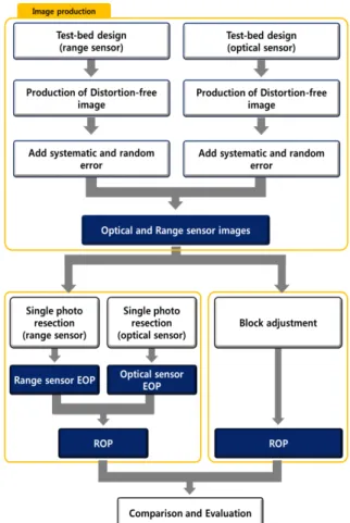
Figure 1. is flow chart of this study. This study was proceed to 2 steps. First, system calibration simulation was done, and its results were reflected to real system calibration. Second, real system calibration was carried out. And its results were evaluated and compared with results of simulation. Furthermore, in this study, before performing experiments, testbed for optical and range sensors system calibration were designed, and manufactured
This contribution has been peer-reviewed.
.
Figure 1. flow chart of study
2.1 Used Sensor
In this study, Optical and range sensors were used for producing sensors system to getting 3D model data. Model name of used optical sensor is CANON EOS 6D body which is equipped 35mm f/2 lens. And Model name of range sensor is SR4000 which is manufactured by MESA imaging company. Table 1. and 2. are each shows specification of optical sensor and range sensor.
Table 1. Specifications of optic sensor body and lens Optic sensor body Optic sensor lens
Model Cannon EOS 6D Model Cannon EF
35mm f/2 IS USM
Image sensor
CMOS (35.8×23.9mm)
Focal
length 35mm Pixel
size 0.00655mm FOV 63°
Table 2. Specifications of range sensor
Model SR4000
Pixel array size 176(h)×144(v)
Pixel size 40
Focal length 5.8mm
RGB images are get from optical sensor and each pixel of image has image coordinates, xopt, yopt. In case of range sensor, it produce two kinds of data. First, range sensor produce single band images, and pixel of this image has image coordinates xr, yr. Second, range sensor produce distance data which are measured between sensor and a objects. And distance data are expressed by 3 dimensional coordinates form (xd, yd, zd). In case of distance data, it is sensitive to color of objects. Because, range sensor measure distance by using infrared ray, and infrared has different reflection characteristics in each color of object. this characteristic is important in testbed design.
2.2 Testbed Design
Testbed was designed with consideration below. i) After image data are produced, testbed should be covered most space of image. ii) Even if distance(between sensors and testbed) change under predetermination range, Sufficient GCP(Ground Control Points) should show in image. iii) making flat and Non-flat type testbeds for checking influence by testbed type changing. iv) And characteristics of each sensors.
Full size of testbed is 4.9×4 meters, and it is consists of 0.7×0.5 meter sized rectangles. GCP for optical sensor are located in edge of rectangles(Figure 2.) and each GCP has 3D coordinates Xopt, Yopt, Zopt. Test-bed for optical
sensor was designed to 3 type. i) Type 1 is flat shape test-bed. ii) In case of Type 2 test-bed, there are points which has 0.25m height. iii) and Type 3 test-bed has points which has 0.5m height. The points marked in a diamond pattern(Figure 2.) are the spots that is located on the same plane as the test-bed. The points in a circle are offset from the plane of the test-bed by 0m (type 1), 0.25m (type 2), and 0.5m (type 3).
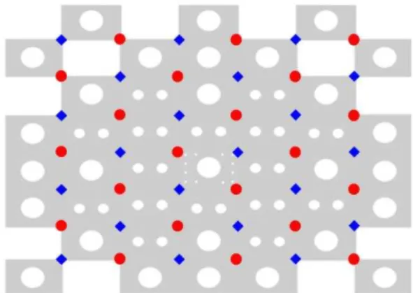
Figure 3. shows design of range sensor test-bed. A white circles were put against a black rectangle for a test-bed of the range-sensor (Derek et al., 2010). The GCP are located in center of the circle and has 3D coordinates Xr, Yr, Zr. There are three kinds of circles in the test-bed, and they have three kinds of diameter(4cm, 16cm and 28cm).
Figure 2. Test-bed design (diamond shape: points which are not given changing in height / circle shape : points
which are given changing in height)
Figure 3. Test-bed design for range sensor
2.3 Mathematical Model (between sensors and GCP)
Relation between GCP and data of each sensors are explained by mathematical. Mathematical models of optical sensor are i) collinearity equations(Equation 1 and 2) ii) and distortion equations(Equation 3 and 4). First, collinearity equation explain relationship between image coordinates of optical data and GCP. Second, Distortion equation explain distortion which is in optical data.
x − ∆x − �= − −− ++ −− ++ −− (1)
y − ∆y − �= − −− ++ −− ++ −− (2)
where x, y = image coordinates of sensor data
This contribution has been peer-reviewed.
∆x, ∆y = distortions of image coordinates xp, yp = principal points of image data f = focal length
m11~m33 = components of rotation matrix X, Y, Z = ground coordinates of control points X0, Y0, Z0 = exterior orientation parameters
∆x = x̅ K r + K � + K �6 + � � + 2 x̅ +
2� ̅ ̅ + � ̅ + � ̅ (3)
∆y = x̅ K r + K � + K �6 + � � + 2 y̅ +
2� ̅ ̅ (4)
where x̅ = x − �
y̅ = y − yp
K1 ~K3, P1, P2, A1, A2 = distortion parameters
Mathematical models of range sensor are i) collinearity equation (Equation 1 and 2), ii) range value equation (Equation 5) iii) and distortion equation (Equation 3, 4 and 6). First, collinearity equation of range sensor is same as optical sensor's. Second, range value equation explain euclicean distance between center of range sensor and GCP. In case of range sensor, there are three kinds of distortion equations. First and second distortion equations of range sensor are same as optical sensor's. Last one explain istortion of range value (Equation 6).
ρ − ∆ρ = √ − + − + − (5)
where ρ = range value(measured distance value)
∆ρ = distortion of range value.
∆ρ = d + ρ + ∑ [ �sin ��
� ρ ] + e ̅ + ̅ + �=
� + � + ∑ = ∑ = + − ̅ − ̅ (6)
where d0~d6, e1~e10 = distortion parameters
3. SIMULATION
Figure 4. is flow chart of simulation. Simulation consists of steps which are i) predetermination of parameters, coefficients and shooting location, ii) image production, iii) system-calibration with single photo resection and block adjustment methods, iv) and comparison of the results.
3.1 Pre-Determination and Simulation Data making
Before performing system calibration simulation, there are several things which must be determined. In system calibration, mathematical models are used, and they includes each sensor's EOP(exterior Orientation Parameters), IOP(Interior Orientation Parameters), distortion parameters and ROP(Relative Orientation Parameters).
EOP are location of sensor which are expressed by ground coordinates. In this study, location of sensors were set as in Figure 5. The circle shows the location of optical sensor, the rectangle, the range sensor.
Figure 4. Flow chart of system calibration simulation
Figure 5. Shooting location of optical and range sensors in simulation (circles : optical sensor / squares: range sensor)
IOP and Distortion parameters relate with each sensor, and these were pre-set as Table 3 and 4. In this study, optical and range sensors are fixed on a 0.4m-long frame, and the angle between the sensors was set at 6° in a counter-clockwise direction from the Y axis (Figure 6). ROP of range sensor can be calculated by plotting the location relationship between the cameras on optic-sensor coordinates (Table 5).
This contribution has been peer-reviewed.
Table 3. Interior orientation parameters of optical and range sensors
Principle point x
(mm)
Principle point y
(mm)
Focal length
(mm) Optical sensor 0.003 0.003 35 Range sensor 0.786 0.2166 5.8
Table 4. Distortion parameters of optical and range sensors
Optical sensor Range sensor
Value Value value
k1 -3.30E-04 k1 -7.81-E03 d0 -4.6266
k2 0 k2 -2.72E-04 d1~d7 0
k3 0 k3 0 e1~e11 0
p1 0 p1 -1.15E-04
p1 0 p1 -2.87E-04
a1 0 a1 0
a2 0 a2 0
Figure 6. Relative location between sensors
Table 5. Relative orientation parameters of range sensor
X0 (m)
Y0 (m)
Z0 (m)
ωrop
(degree)
φrop
(degree)
κrop
(degree)
0.39945 0 -0.02093 0 6 0
After predetermination, simulation data were made. One data-set include optical Image, Image of range sensor and distance data of range sensor. And data-set was produced per each EOP. As a result, 21 data-sets were produced at 21 locations.
3.2 System Calibration Simulation
Purpose of simulation was to find efficient method of system calibration. For this purpose, simulation was designed by considering following variables, i) system calibration method, ii) testbed type, iii) and distance data(whether use it or not).
First, two kinds of method were used in system calibration. First one was one step method which is based on bundle adjustment method, and the other one was two step method which is based on single photo resection. Second, in this study, 3 type of testbed were used to simulation. Lastly, distance data is not essential option to perform system calibration. So, system calibration can be done without distance data. In this study, two kinds of system calibration were done. One was done without including distance data, and the other was done by using distance data.
3.3 Results of Simulation
Figure 7. shows the results of system calibration. Generally, one step method(block adjustment) shows better accuracy in all cases. And especially, case which was used one step method and distance data shows most accurate results. Generally, type of testbed do not give effect to system calibration accuracy, except φ of case which was used two step method without distance data. Therefore, testbed type give effect to φ, but its influence is very small. Distance data give a big impact on accuracy of result, in case which was used two step method. And its accuracy shows very similar level to results of one step method.
Figure 7. Comparison of relative orientation parameters errors
((a) X0, Y0, Z0 / (b) ω, φ, κ)
4. SYSTEM CALIBRATION
Figure 8. Flow chart of real system calibration
This contribution has been peer-reviewed.
In this study, results of simulation were reflected in real system calibration. So only type 1 testbed were used in real system calibration. In real system calibration, effects from i) system calibration methods, ii) distance data(range data) and iii) quantity of data were calculated and compared with results of simulation.
Figure 8. is flow chart of real system calibration. Real system calibration consists of steps which are i) making real testbed, ii) acquisition sensors data, iii) system-calibration with single photo resection and block adjustment methods iv) and comparison of the results.
4.1 Manufacturing Testbed and Data Acquisition
Figure 9. Testbed for system calibration between optical and range sensor
Figure 10. Optical and range sensor system(left), measuring GCP by using total station(right)
Figure 11. Shooting location of optical and range sensors (circles : optical sensor / squares: range sensor)
Testbed was made with based on testbed design which was used in simulation (Figure 9). Figure 10(left) shows sensor system which is consist of optical and range sensor. By using this sensor system, image and distance data were acquired in each shooting location(Figure 11). Meanwhile GCP(Ground Control Points) were acquired by using total station(Figure 10(right)).
4.2 Results of System Calibration
Table 6. Two step method results (single photo resection) Used
data X0 (m)
Y0 (m)
Z0
(m) (degree) ω (degree) φ (degree) κ
Image 0.4311 0.0397 0.0923 1.8574 2.9465 0.2011
Image
Distance 0.4153 0.0192 0.0441 1.3605 2.6433 0.2652
Table 7. One step method results (bundle block adjustment) Used
data X0 (m)
Y0 (m)
Z0
(m) (degree) ω (degree) φ (degree) κ
Image 0.4636 0.0538 0.0814 0.6023 5.3842 -0.4660
Image
Distance 0.4190 0.0262 0.0977 0.7467 5.1244 -0.3910
Table 6. and 7. shows results of real system calibration. In case of real system calibration, True value of ROP cannot be acquired. So, Accuracy of ROP is evaluated in an indirect way. In this study, ROP was set approximate value to value of Table 5. This results shows i) Distance data can be improved accuracy of system calibration. And its influence is more significant in real system calibration. ii) In case of system calibration by using distance data, accuracy of X0, Y0, Z0 shows very similar level regardless of methods(one step or two step method). But accuracy of
angle(ω, φ and κ) shows more higher level, in case of using one step method(BBA).
Figure 12. Standard deviation (one step method, piling image)
Figure 12. shows standard deviation of ROP in case of piling images and using one step method. It shows that the more data used, the lower standard deviation value was derived. Because lower standard deviation means more higher precision, Figure 12. can be interpreted that quantity of data relative to system calibration accuracy. And this trend continued until data piling up to 4m region.
This contribution has been peer-reviewed.
5. CONCLUSION
Purpose of this study is finding efficient methods of system calibration between optical and range Sensors. For this purpose, this study was proceed to following steps. First, testbed which is optimized to system calibration between optical and range sensors was designed and manufactured. Second, system calibration simulation was performed to find more efficient real system calibration experiment. Third, real system calibration was performed and its results was evaluated and compared.
Finally, efficient system calibration methods could be found as the follows. i) One step method (bundle block adjustment) shows better results in accuracy than two step method (single photo resection). ii) Distance data give significant contribution to the accuracy of ROP. iii) More efficient experiment can be done by using acquired data in the location which is 2~4m away from testbed (in this study, total 12 data set). In future study, study about data fusion and 3D indoor model will be performed by using ROP which was derived in this study.
ACKNOWLEDGEMENTS
This research was supported by Basic Science Research Program through the National Research Foundation of Korea(NRF) funded by the Ministry of Education, Science and Technology(NRF-2012R1A1A1044722)
REFERENCE
Choi, J. and Sohn, K., 2011, Multi-view depth image resolution enhancement based on view coherence, 2011 Conference of The Korean Society of Broadcast Engineers, The korean society of broadcast engineers, July, Korea, pp. 373-375.
Habib, A.F. and Morgan, M., 2005, Stability analysis and geometric calibration of off-the-shelf digital cameras, Photogrammetric Engineering and Remote Sensing, Vol. 71, No. 6, pp. 733–742.
Habib, A.F., Morgan, M., and Lee, Y., 2002, Bundle adjustment with self-calibration using straight lines, The Photogrammetric Record, Vol. 17, No. 100, pp. 635–650. Habib, A.F. and Morgan, F.M., 2003, Automatic calibration of low-cost digital cameras, Optical Engineering, Vol. 42, No .4, pp. 948–955.
Kang, Y. and Ho, Y., 2011, Depth generation method using multiple color and depth cameras, Journal of the Institute of Electronics Engineers of Korea, Vol. 48, No. 3, pp. 326– 331.
Kim, C., Sohn, H., Heo, J., and Lichti, D., 2011, 3D range camera calibration, 2011 Conference on Geospatial Information, Korean society for geospatial information system, May, Korea, pp. 127-128.
Lee, C., Kim, C., and Seo, S., 2010, Platform calibration of an aerial multi-view camera system, Journal of the Korean Society of Surveying, Geodesy, Photogrammetry and Cartography, Vol. 28, No. 3, pp. 369-375.
Lichti, D.D. and Kim, C., 2011, A comparison of three geometric self-calibration methods for range cameras, Remote Sensing, Vol. 28, No. 5, pp. 1014-1028.
Lichti, D.D., Kim, C., and Jamtsho, S., 2010, An integrated bundle adjustment approach to range camera geometric self-calibration, ISPRS Journal of Photogrammetry and
Remote Sensing, Vol. 65, Issue 4, pp. 360-368.
This contribution has been peer-reviewed.