Portifolio selection with random transaction costs

~ ~

#"FUNDAÇAo

,

GETULIO VARGAS

SEMINÁRIOS

DE PESQUISA

ECONOMICA

•

•

•

...

EPGE

Escola de Pós-Graduação em Economia

··Portfolio Selection with

I

~andom

Transaction Costs"

\

Professor: Marcelo Nazareth (The University of Chicago)

LO .. AI.

Fundação Getulio Vargas

Praia de Botafogo, 190 - 10

0

andar - Auditório Eugênio Gudin

BAlA

11/0512000 (58 feira)

tloltA

ItlO

16:00h

•

Portfolio Selection

with

Random Transaction Costs

Marcelo N azareth

*

Second Draft

March 26, 2000

Abstract

Transaction costs have a random component in the bid-ask spread. Facing a high bid-ask spread, the consumer has the option to wait for better terms oI' trade, but only by carrying an undesirable portfolio bal-ance. We present the best policy in this case. We pose the control problem and show that the value function is the uni que viscosity solution of the rel-evant variational inequality. Next, a numerical procedure for the problem is presented.

,

"

1 Introduction

The literature of portfolio selection in a continuous time setting starts with Merton [26J. Merton shows that in the absence of transaction costs, the best strategy for the investor is to keep his holdings in the stock and in the money market account at a constant proportion. To implement this strategy the in-vestor should trade continuously. The first objection to this setup, is that this strategy breaks down in the presence of an arbitrarily small transaction cost. The wild nature of the Brownian motion that drives the stock price movements implies that the strategy has infinite cost. The first model with fixed trans-action costs was developed by Constantinides [5J. He shows that the investor couple with transaction costs by refraining to transact too often. The optimal strategy is to transact only when the proportion of stock relative to bonds in the portfolio gets too high or too low. Constantinides also reports that the loss in consumption relative to the Merton paradigm is small. With a 2% transaction cost consumption decreases by 0.4%; with 5% consumption decreases by 1%. Formal proofs of the results in the Constantinides paper can be found in Davis and Norman [7J . For a rather different proof of the same results see Fleming and Soner [12J pg. 342. Were not for the development of the notion of viscosity solutions (see [6J and [12]), anything slightly more complex than the Constan-tinides model would become impossible to analyze. After the breakthrough, more complex models appeared. Fleming and Zariphopoulou [13J analyzed a model with different borrowing and lending rates, Zariphopoulou [32J studies a model with transaction costs and borrowing constraints. For a model of option pricing with transaction costs, see Davis, Panas and Zariphopoulou [8J. A com-mon characteristic of ali the models above is the nature of the optimal policies. The optimal police implies that there is a region where it is optimal not to transact. As soon as the stock holdings try to escape out of this region, the controller is to purchase or sell stock, so as to keep the holdings just within the prescribed region. This paper is a first attempt to look at these policies in the presence of random transaction costs.

Transaction costs faced by consumers usually have a fixed component like brokerage fees, as well as a random component in the form of the bid-ask spread. Furthermore , the bid-ask spread can be viewed as a measure of market liquidity. Suppose large shocks hit the market making the controllers portfolio unbalanced. Suppose also that the market lost liquidity so that the bid-ask spread is tem-porarily high. Should the controller pay high transaction fees and rebalance the portfolio at once, or exercise his/her option and wait for better terms of trade? This paper is able to give a definitc answer to this question: Do wait.

,

•

rule rather than the exception. Many branches of the market microstructure literature links high volatility in the market with high bid-ask spreads. We have attempted to build this feature in our mo deI. This attempt was not fully successful. The readers can judge by themselves by reading the next section.

The paper is organized as follows: Section 2 develops the dynamics of the transaction costs. Section 3 poses the control problem and proves some elemen-tary properties of the value function. Section 4 establishes the value function as the unique viscosity solution of the relevant Hamilton-Jacobi-Bellman equation. Section 5 deals with utility function in the HARA class. Section 6 deals with the numerical solution of the model. Section 7 presents the numerical results and conclude. The elementary proofs are in the appendix.

2

Modeling Transaction Costs

In the model, the agent faces a decision of purchasing and selling stock. He faces proportional transaction costs which are random. When he purchases y dollars worth of stock, his money market account is debited y(l

+

Kd dollars. When hc sells y dollars worth of stock, his money market account is credited y(l

+

Kd-1 dollars. I will be looking for a process Kt which is nonnegative. In this section I develop the dynamics for the stock price St and transaction cost

Kt· I approach this problem by first developing a discrete time model, where intuition is easicr to grasp. The discrete time model is only a device to capture some stylized facts. In the second subsection I proceed to take it's continuous time limito In later sections, I will only work with the continuous time processo

2.1

Discrete Time Model

I start with a discrete time, standard log-normal process for the stock price. For m

=

0,1,2, ... define

(1)

So given ,Zm i.i.d. N(O, 1)

I

maker an abnormal flow of buy orders. He, in turn, will respond by increasing the bid and ask prices, as well as by widening the spread. The overall effect is a positive association between the size of the spread and the absolute value of the stock price change. The effect also tend to be temporary, in the sense that, once the market maker learns the information conveyed by the flow of orders, the spread is reduced. Empirical tests of the results above have been carried out by Bollerslev and Melvin [3], Hasbrouk [15] and Hausman, Lo and MacKinlay [16J. Hasbrouk finds evidence linking large trades with wide spreads, what is consistent with the Easley and O'Hara mo de!. Hausman, Lo and MacKinlay find positive links between stock price volatility and bid-ask spreads in the D.S .. The same relationship was uncovered by Bollerslev and Melvin in foreign exchange data. The idea, hence, is that transaction costs are higher when the market is volatile. A sequence of abnormally large shocks hitting the market are supposed to make transaction costs grow temporarily. A calm period, in the other hand, should make transaction costs smaller. The situation is reminiscent of a ARCH like modeling. I assume that current transaction costs Km+! depends only on the past shocks (Zm,Zm-!,"') and that (Km+!,Zm+l) is markovian.

What are the features I want from the function g? Well, if

IZml

is large, I want Km+! to increase, at least temporarily. Whereas, if

IZml

is small, I want

Km+l to decrease. On top of that, I also want the flexibility to let transaction costs respond asymmetrically with respect to positive and negative shocks. Like the EGARCH model, I assume that a large negative shock increases transaction costs more than a shock that is equally large but positive. The rational in the EGARCH model is to capture the so called "Ieverage effect". Here, it just means that it is particularly expensive to transact during crashes.! Summing up:

{

If Zm is largc and positive ~ If Zm is small ~

If Zm is large and negative ~

Km+l

t

Km+l..l-Km+l

tt

Before I proceed, I should warn the reader that the situation is only analo-gous to ARCI-! modeling. In my mo deI the volatility of the stock prices is always constant. I completely abstract from stochastic volatility considerations, trying to isolate the effect of random transaction costs.2 _{First, I specialize thc function}

g(Zm,Km). With a view toward the continuous time limit I pick the "square root" processo

Km+I Km

+

fJ(o. - Km)

+

À

Pm

x

---~--- (2)

1 No empírical evídence to support thís partícular feature will be presented. This just gives me exlra fiexíbilíty and can be easily undone by settíng lhe parameter p, below, appropriately.

,

'"

Ka given

the constants satisfy,

.

'

!

.

"

a,(3,).,>O

-1

<

p

<

1

2 (3

a>

).,2

2

'Y

= (

1 - P )1/2

1 - 2j-rr

,

o __ •.•.• '. ___ •..• ,. ___ •.••.• ___ •.•

-~!-, ---::-,:-, --:;;';",---;;;,,--;-0'''", ----'O~-;;':'.2,---;;;"--;''''" .• --::,:-, ---.J lSI'1oci<

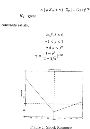
Figure 1: Shock Response

The response of Km+I/ JKm+1 to shocks Zm are plotted in figure 1 for

p

<

O. I favor the case p

<

O. The choice of the process Km is had-oc. It is

dictated, however, by thc desired responsc to shocks described above as well as by the properties of the continuous time limit of the system (1-2).

2.2

Continuous Time Model

I now turn to the continuous time limit of the system (1-2). All the missing details can be found in Nelson [27], which I follow closely. I will be considering 3 kinds of processes (where X stands for S, K and Z).

• Sequences of discrete time processes {Xt;,h} that depend on h and the discrete time index mh, m

=

O, 1,2, .... I set X~

=

X_a Vh.

• Sequences of continuous time processes {X th } defined as

ph[X;

=

Xt;,h , mh ::; t

<

(rn

+

l)h]

=

1

,

•

• Limit diffusion processes

{Xt}

to which

{Xn

will converge weakly as

h..(.O.

Now rewrite the system (1-2) as

Sfm+1)h

=

S:;'h

+

J.l S:;'h h

+

(j S:;'h Z:;'h

Kfm+1)h

=

K:;'h

+

fJ(a - K:;'h)h

+

À

J

K:;'h X X

[p

Z;:." +1' (IZ;:'hl- (2h/11')1/Z)]

(S~, K3)

(So,

K

_o)

given

Z:;'h i.i.d. N(O, h)

(3)

(4)

The following proposition is an easy consequence of theorem 3.1 in Nelson. It's proof is in the appendix

Proposition 1 (St, Kth) =:::} (St,Kt ) (weakly) as h..(. O. Where (St,Kd sat-isfy:

dSt

=

J.lSt dt

+

(j St dWl,t

dKt

=

fJ(a - Kt) dt

+

À"fi(;

dW2,t

So, Ko

given

and

[R\,l

Wz,tl

is a 2-dimensional standard Brownian motion satisfying

[ dW1 t ] [ , dW

1

(1

p)

2:t dR 1,t dW2,t

=

p 1 dt.

(5)

(6)

Intuitively, (stm+l)h - S:;'h) , (Ktm+l)h - K:;'h) and h , are the discrete time counterparts to dS, dK and dt, respectively. Perhaps it is not so easy to see that

Z:;'h and p Z:;'h +1' ( IZ:;'hl- (2 h/11')1/2) are also the discrete time counterparts of [dW1,t dW2,t].

The reason this holds, is because if I define for each m

=

1,2, ... and eacil

t E [0,1]

[mil

Qm,t

==

(1 - 2/11')-1/2 2)IW(j+1)/m - Wj/ml- (2/11'm)1/2}

j=l

,

,

•

Wt'

a 2-dimensional Brownian motion on [0,1]. Qrn,t depends on the whole path of W. for s ~ t. But as m

-+

00, Qm,t converges in distribution to a Brownian motion independent of Wt . The way to get a sequence of processes that converges to a Brownian motion that is correlated with W_t is by taking a linear combination of Wt and Qrn,t. I claim that the choice of a square root process for the transaction costs is reasonable. With this choice, I get a process

Kt that

• Is stationary.

• Is positive with probability 1.

• It mean reverts, and when properly initialized, the mean of Kt is equal to

the mean reversing point a.

The last property leads to a very natural way to access the effects of random transaction costs as opposed to fixed transaction costs. Namely, I will be com-paring the effects of fixed costs [( 1

+

a), (1

+

a)

-1]

as opposed to random costs [(1

+

K t ), (1

+

Kt)-l] initialized at Ko

=

a. Things are not as nice as they look, however. This setup has a drawback and is to be regarded as a first attempt to modeling random transaction costs. The reason being that all the nice intuition of the discrete time model 1-2 have vanished out of thin air. The continuous time model 5-6 has only a fiavor of the association between transaction costs and volatility. In the limit all that remained was a negative association between prices and transaction costs (if p

<

0).3 The natural way to recover the nega-tive correlation would be to regard Kt as having the double role of stochastic volatility and transactiou costs as in

So,Ko given

[ dW1,t ] [ _dWz,t dWl.t

(7)

(8)

The drawback of this alternative setup is two-fold. The first is the increase in complexity, which can be severe. The second is the difficulty of interpretation. Whatever rcsults I get with the setup 7-8, canuot be attributed separately to stochastic volatility or random transaction costs. I will stick to the setup 5-6,

which is much simpler and can be more easily interpreted. In the end of section 4, I comment on what remains true with the alternative setup 7-8.

3The easiest way to see this is the case, is by considering a standard Euler approximation for the system 5-6. Approximating (W1,t, W2,,) by correlated normaIs (Zl' Z2) one sees that

,

,

3

Investment-Consumption Model

In the first sub-section pose the control problem for the consumer and establishes some properties of the value function. In the second sub-section, I write down the Hamilton-Jacobi-Bellman equation, the value is supposed to satisfy.

3.1

The ControI FormuIation

The market has 2 securities. The first is a risk free money market account, which pays a constant interest rate r

B(t)

=

ert (9)

The second security is a stock 5(t). It's dynamics is given together with the dynamics of the transaction costs K(t) by

(10)

(11)

50, Ko given

[ dWTl,t ] [ _dTh,t dW1,t (12)

[W1,t W2,t

1

is a two-dimensional Brownian Motion on a complete probabil-ity space

(n,

Ft, F, P). Ft is the completion of a(W1,t, W2,t; s ~

t) .

The amounts held in the money market and stock accounts are denoted X(t)

and Y(t) respectively. The consumer chooses processes (C(t), L(t), M(t)).

• C(t) is the dollar consumption processo

• L(t) is thc cumulativc dollar transfer into the stock account.

• M(t) is the cumulative dollar transfer into the money market account.

Transfers between the stock account Y

(t)

and the money market account

X(t) incur transaction costs (1

+

K(t)). More specifically, a instantaneous

transfer into the stock account of size dL(t) reduces the bond account by (1

+

K(t))dL(t). A instantancous transfcr out of the stock account of size dM(t)

increases the bond account by (1

+

K(t))-ldM(t). My bookkeeping always penalizes the money market account.

The consumption process C(t) drains directly the bond account. Transfers out of the money market account to consumption incur no transaction costs.

•

,

•

X(t)==x+ lt(rx(s)-c(S))ds - lt(l+K(S))dL(S)

+ l t (1

+

K(s))-ldM(s) (13)

Y(t) == Y

+

l t 11 Y(s) ds

+

l t (j Y(s) dW1,s

+

L(t) - M(t) (14)

K(t) == k

+

l t !3(a - K(s))ds

+

l t À v'K(s) dW2 ,s (15) The investor has Von Neumann-Morgestern preferences

over the consumption process {C(t)j t

:2:

O} . ó is the subjective discount factor and U(C(t)) has the following properties:

• U: R+ I-t R , U E C2 with U(O) == O ,U'

>

O , U"

<

O.

• O ~ U(c) ~ M (1

+

cp

for some M

>

O, 'Y E (0,1)

• U satisfy the Inada conditions U' (O)

==

00, UI (00)

==

O

The investor faces the following problem. Given (X(O)

==

x, Y(O)

=

y, K(O)

==

k) maximize

V(x,y,k)

==

sup E(x,y,k)

[1

00

e-ot U(C(t)) dt]

A("y.k) o

(16)

A(x,y,k) is the set of triples (L(t), A1(t), C(t)) satisfying

A-I (L(t), M (t)) are right continuous, adapted, non-decreasing processes. I set

L(O)

=

M(O) == O.

A-2 C(t) is adapted, continuous, non-negative and

10

00

C(t)dt

<

00.

A-3 X(t), Y(t)

:2:

o,

A-3 is admittedly restrictive. It does not allow leveraged or short positions in the stock. One excuse is that the parameters in the numerical computations will be such that the consumer never let X(t) ~ O ar Y(t) ~ O.

The real reason, however, is that the natural alternative assumption leads to a pathology. It would be natural to assume instead

_ { X(t)

+

Y(t)(l

+

K(t))-l if Y(t)

:2:

O

•

,

this says that, should the investor be called upon liquidating his position in the stock, at current transaction cost, he remains solvent.

But consider two sequences ofpoints an

=

(xn,Yn,kn)

=

(11,,-1/11,,11,2 -1)

and bn

=

(11,,0,11,2 - 1). Along bn the consumer gets infinitely rich. It is feasible never to transact and consume arbitrarily large amounts directly from the money market account. Along an he is always broke. The only feasible strategy is to liquidate his stock position immediately and consume zero forever. Acting otherwise risks making Z(t)

<

O which is not allowed.

The pathology is that you may have an arbitrarily small short position in the stock (-1/11,) but transaction costs are so high (11,2 -1) that you are in fact insolvent. Thisimpliesthat lan-bnl-+ Obut lV(an)-V(bn)l-+ U(oo)-U(O)

>

O. This shows that under Z

2':

O the value function is not uniformly continuous, a property that is essential for my uniqueness resulto

I will assume that the problem 16 has a solution. As usual, if the param-eters are set arbitrarily, investing everything in the stock, followed by massive consumption achieves an arbitrarily large value. I assume this is not the case. One possibility is to set the parameters as in the Merton problem.

I dose this section proving some clementary properties of the value function. The proof is in the appendix.

Proposition 2 (a) V(x,y, k) is concave in (x,y).

(b) V(x,y,k) is strictly increasing in (x,y), non-increasing in k.

(c) V(x, y, k) is uniforrnly continuous.

3.2 The H-J-B Equation

In this sub-section I develop an heuristic argument that suggests that the value function satisfy equation 20 below. The argument is heuristic because it assumes a priori that V (x, y, k) E C2

. It turns out that the value function will satisfy 20 only in a wcak (viscosity) SCllse.

Consider the following strategy: Sell é worth of stock instantly alld continue

optimally thereafter. This implies that we jump from position (x, y, k) to (x

+

E(l+k)-l,y-E,k). Hence

V(x,y,k)

2':

V(x+t(l+k)-l,y-E,k)

Dividing by E and letting é

-l-

0, I get

ôV _ (1

+

k)-l ôV

>

°

,

Analogously, buying E worth of stock instantly and proceeding optimally thereafter yields

V(x, y, k)

2:

V(X - E(1

+

k), y

+

E, k) which implies,

oV

oV

(1

+

k) ox - oy

2:

O

Before I derive the last equation, let me introduce some notation. Let

g(x,y,k)

= [

:~

1 '

f3( Q - k)

E(y,k)

=

dV=[~~l,

8k

)..pCJVky

1

)..2k

D2V

=

[~

t:~~

l.

82_{V 8}2_V 8y8k 7fk'I"

and

(18)

Notice that D2V is not the Hessian matrix of V, since it does not include partials with respect to x.

Last, consider the strategy

S:

In

[O,

t) do not transact and consume at a constant rate c; thereafter proceed optimally. This yields

V(x,y,k)

2:

fot

e-à. U(c) ds

+

ES [e-à! VS(X(t), Y(t),K(t))]

where ES[e-Pt V(X(t), Y(t), K(t))] means that we let the system 13-14 evolve freely, just draining the money market account at rate e. By Ito's lemma

ES[e-à! VS(X(t), Y(t), K(t))]- V(x, y, k)

- ri e-à8_{(_6 V}

₊

_{gT dV}

₊

_{lTr E D}2_{V - e av )ds}

- Jo 2 ' 8x

Hence

l

i 1

oV

o e-às( -6 V

+

9 T dV

+

"2

Tr E.D2V

+

U(e) - c ox )ds ::; O

dividing by t and letting t .). 0, I get "ie

2:

0,

T 1 2 OV

-6 V

+

9 dV

+

"2

Tr E.D V

+

U(e) - c ox ::; O

which implies

-6 V

+

9 T dV

+

~Tr

E.D2V

+

max{U(c) - c

~V

} ::; O (19)

•

,.

Finally we define the operator L by

1

av

L V(x,

y,

k)

==

-6

V

+

9 T dV

+

-Tr 2:.D2V

+

max{U(c) -

c-a },

2 c;::: O x

combine equations 17-19 above to get

.

av av av

_lav

mm{ -L V , (1

+

k) OX -

ay , ay -

(1

+

k) ox}

=

O (20)

The form of the equation 20 suggests that the (x, y, k) space will split in three regions.

(NT)

Where L V

=

O. Here it is optimal not to transact.

(BS)

Where (1

+

k)Vx - Vy

=

O. Here it is optimal to buy stock immediately,

forcing (x,y,k) to return to the boundary ofthe (NT) regíon.

(SS)

Where Vy - (1

+

k)-l Vx

=

O. Here ít is optímal to seU stock ímmedíately, forcíng (x,y,k) to return to the boundary ofthe (NT) regíon.

The boundaríes between the regíons are not known a príorí and have to be determíned together wíth V(x, y, k).

It ís natural to conjecture that the optimal strategy ínvolves singular con-trols. At tíme O, íf the controller finds hímself eíther at the (BS) or the (SS), he jumps immedíately to the boundary of the (NT) regíon along the lines

x(l

+

k)

=

y and x(l

+

k)-I

= y,

respectívely. Afterwards he exercises the

controls L(t), M(t) just enough to keep (x, y, k) ínsíde the (NT) regíon. The con-trols therefore behave líke the local time of the Brownian motíons (WI,t, W₂

,d.

I will show below that the optímal controls never jumps, except, perhaps at t

=

O.

To fully characterize the optímal controls, one would have to actually solve the variatíonal inequalíty 20 above. Thís task is considered near to impossi-ble with today's knowledge. It is feasible to prove numerícally that the space

(x,y,k) splits in the three regions L V

=

O, (1

+

k)Vx - Vy

=

O and Vy - (1

+

k) - I VX

=

O. However, the behavíour of the optimal control descríbed above wíll

remain a conjecture.

4

The Viscosity Property

,

The theory applies to PDE's of the form F(x, u, Du, D2_u)

= a

_{where F :}

RN x R x RN x RNxN

-+

R, where RNxN denotes the set of symmetric N x N

matrices and u is a real valued function defined in a open subset O

ç

R

N . The theory allows F to be fully non-linear and the solution u to be merely continuous. However F is required to satisfy the monotonicity condition

F(x, r,p, X) ::; F(x, S,p, Y) whenever r::; s and Y ::; X

where

r,

s E R; X,p E R N ; X, Y E RNxN and R NxN is equipped if its usual order. The condition on r and s is named properness, while the condition on X

and Y is referred as degenerate elliptic.

In control problems where state constraints are present the relevant notion is that of constrained viscosity solution. It was introduced by Capuzzo-Dolcetta and Lions [4]. See also Katsoulakis [21].

Definition 1 A continuous function u : O

-+

R is a constrained viscosity

solu-tion of

if

F(x,u(x),Du(x),D2_u(x))

₌

a

1. u is a viscosity subsolution of F

= a

on

n;

that is, if for all'lj; E C2 _(O)

and all points Xo such that u (xo) - 'IjJ (xo) attains a local maximum we have

2. u is a viscosity supersolution of F

= a

on O; that is, if for all'lj; E C2(0)

and ali points Xo such that u(xo) - 'IjJ(xo) attains a local minimum we have

The reader should notice the judicious use of O and

n

in the definition. With this definition in hands I can now establish the following proposition, the proof of which follow the lines of [8, 31, 32]. The argument is nowadays standard.

Proposition 3 The value function V(x,y,k) defined by equation 16 is a con-strained viscosity solution of

. âV âV âV _lâV

m m { - . c V , ( l + k ) - - - , - - ( l + k ) - } = a

âx ây ây âx

Proof. By definition we have to establish the sub and supersolution

proper--3

,

subsolution property Let'IjJ E C2(R~) and Zo

=

(xo, Yo, ko) be a local maxi-mum of V - 'IjJ. Assume, without loss of generality that

V(zo) = 'IjJ(zo) and V ~ 'IjJ on R~ (21)

I need to show that

Suppose to the contrary that

(1

+

ko) â'IjJ(zo) _ â'IjJ(zo)

>

O ,

ox ây (23)

â'IjJ(zo) _ (1

+

kO)-l â'IjJ(zo)

>

O,

ây âx (24)

and

ó 'IjJ(zo) - 9 T (zo)d'IjJ(zo)

- 2

1 Tr I:(yo, ko).D 'IjJ(zo) 2 â'IjJ(zo) - max{U(c) c

-â- }

>

e

c~O x (25)

for some ()

>

O.

Since 'I/J and U(c) are smooth these inequalities also hold in a neighborhood of Zo, That is, there exists

e

>

O and a radius r

>

O such that for all

z

=

(x,y,k) with z E B(zo,

r)

(1

+

k) â'IjJ(z) _ o'IjJ(z)

>

O ,

âx oy (26)

o'l/J(z) _ (1

+

k)-l â'IjJ(z)

>

O

ây

OX

(27)

and

1

Ó 'IjJ(z) - 9 T (z)d'IjJ(z) -

2Tr

I:(y, k),D2'IjJ(z)

_ o'IjJ(z)

- max{U (c) -

c-â- }

> ()

(28)

c;::': o x

Next I need the following auxiliary result, which says that the optimal trajectory has no jumps at t

>

0+, Let the optimal trajectory be Zô(t)

=

(Xô(t), Yo*(t), Ko(t)); where optimal controls (C*(t), L*(t), M*(t)) are

Lemma 1 Assume inequality 23 holds (resp. 24). Let A(w) be the event that the optimal trajectory has a jump of size f along the direction (1

+

ko,l,O) (resp. direction((l+ko)-I,-l,O)).

Assume that ajter the jump the state is (xo - (1

+

kO)f, Yo

+

f, ko). Then,

((1

+

ko/~(zo)

_

â~(zo))P(A)

:::;

O.

âx ây

which implies P(A)

=

O.

Proof. By the dynamic programming principIe

so,

V(xo, Yo, ko)

=

EV(xo - (1

+

kO)f, Yo

+

f, ko)

=

i

V(xo - (1

+

kO)f, Yo

+

f, ko) dP

+

r

V(xo, Yo, ko) dP

líl-A

o

i

V(xo - (1

+

kO)f, Yo

+

f, ko) - V(xo, Yo, ko) dP

<

i

~(xo

- (1

+

ko}t:, Yo

+

f, ko) -

~(xo,

Yo, ko) dP

hence,

O:::; Iim sup

r

~(xo - (1

+

kO)f, Yo

+

f, ko) - ~(xo, Yo, ko) dP

,~o

lA

f

By Fatou's Iemma

o

<

r

limsup~(xo-(l+ko)f,Yo+f,ko)-ijJ(xo,Yo,ko) dP

lA

,~o

f

r

-(1

+

kol â'ljJ(zo)

+

â~(zo)

dP

lA

âx ây

(-(1

+

ko)

â~(zo)

+

â~(zo))

P(A)

âx ây

The same argument hoIds for the other inequality.

Continuing the proof of the proposition, define the stopping time

T

=

inf{t ~ O: zt(t) ~ B(zo,r)}

•

28 to get

E f; () e-6tdt

<

E f; e-6t [81j;(Zô(t» - 9 T (Zô(t»d1j;(Zô(t»

- ~ Tr 'E(Yo*(t), Ko(t) ).D21j;(Zô(t»

-U(C*(t»

+

C*(t) ô1/J(;~(t))

1

dt

+

E foT e-6t_rô

1/J(;i(l)) - (1

+

KO(t»-l Ô1/J(;~(t))l dM*(t)

(29) Denote the terms on the left hand si de by

E 11 (r) - E foT U(C*(t» dt

+

E 12 (r)

+

E 13 (r) (30)

Applying !to's formula for semi-martingales yields

To get the desired result, just combine 29 , 31 and 1j;(zo)

=

V(zo)

<

1j;(zo) - E {e- ÓT 1j;(Zt(r»} - E foT U(C*(r» dt

V(zo) - E {e-ÓTV(Zt(r»} - E foT U(C*(r» dt

O

which is a contradiction with ()

>

O and r

>

O a.s. The equalities follow from the optimality of Z*(t) and the dynamic programming principIe. So, at least one of the arguments inside the min operator must be non positive, what establishes the subsolution property.

supersolution property Let 1j; E C2(R~+) and Zo

=

(xo, 1/0, ko) be a local minimum of V -1j;. Assume, without loss of generality that

V(Zo)

=

1j;(zo) and V ~ 1j; on R~+ (32)

I need to show that

I will prove that each term inside the min operator is nonnegative.

,

•

from position (xo, Yo, ko) to (xo

+

f(l

+

kO)-l, Yo - f, k). Hence

'Ij;(xo, Yo, ko)

=

V(XO, Yo, ko)

>

V(XO

+

f(l

+

kO)-l, Yo - f, ko)

>

'Ij;(XO

+

f(l

+

kO)-l ,Yo - f, ko)

dividing by f and letting f

+

O, I get

Analogously, starting at Zo , buying t worth of stock instantly and pro-ceeding optimally thereafter yields

'Ij;(xo, Yo, ko)

=

V(xo, Yo, ko)

>

V(xo - t(l

+

ko), Yo

+

t, ko)

>

'Ij;(xo - f(l

+

ko), Yo

+

f, ko)

which implies

(1

+

ko) à'lj;(xo) _ à'lj;(zo)

>

O

àx à y

-Last, consider the strategy S: In [O, t) do not transact and consume at a constant rate c; thereafter proceed optimally. This yields

'Ij;(zo)

=

V(zo)

>

fot e-os U(c) ds

+

ES _{[e-ot VS(X(t), Y(t),K(t))]}

>

fot e-os U(c) ds

+

ES

_[e-

ót _{'lj;s(X(t), Y(t),K(t))]}

where ES[e- pt VS(X(t), Y(t), K(t))] means that we let the system 13-14 evolve freely, just draining the money market account at rate c. By Ito's lemma

E[e- ot 'lj;S(X(t) , Y(t), K(t))]-'Ij;(xo,yo, ko)

=

J;

e-OS(_ó 'Ij;

+

9 T d'lj;

+

~Tr E.D 2'1j; - c~)ds

hence

l

t 1 à'lj;

e-OS( -p 'Ij;

+

9 T d'lj;

+

-Tr E.D2'1j;(zO)

+

U(c) - c-à )ds::::: O

o 2 x

dividing by t and letting t

+

O, I get "ic

2:

O,

T 1 2 à'lj;(zo)

-15 'Ij;(zo)

+

9 (zo)d'lj;

+

"2Tr E(zo).D 'Ij;

+

U(c) - c~ ::::: O

which implies

1 à'lj;(zo)

-15 'Ij;(zo)

+

9 T (zo)dw

+

-Tr E(zo).D2'1j;

+

max{U(c) c

-à- } ::::: O

2 c20 x

or,

..

..

The last result in this section proves that the value function as defined by equation 16 is the unique constrained viscosity solution of the variational inequality 20. As is common in this theory, the result is stated in the form of a comparison resulto

Proposition 4 Let u be a continuous viscosity subsolution of 20 on R~ and v

be a bounded below, uniformly continuous viscosity supersolution of 20 on R~+. Then u ::; v in R~.

First I construct a strict supersolution of 20 in R~+.

Let WM(X,y) be the solution of the Merton problem, with utility function

UI (c). Assume UICc) ~ U(c) with strict inequality for c

>

O. Then, WM(X, y)

=

vez) where z

=

x

+

y and for z

>

O, v satisfies

{

<5v(z)

= -

(i'2~i

~:~(:?

+

rzv'(z)

+

maxc2:0{U1(c) - cv'(z)}

(34)

vez)

>

O, v'(z)

>

O , v"(z)

<

O

now, define

for (1

+

k)-l

<

a

<

(1

+

k)

then,

aWM aWM

(l+k)a;;-(x,y,k)-ay(x,y,k)

=

(l+k-a)v' (x+ay)

f(x, y, k)

>

o

(35)

aWM _laWM

-a-(x,y,k) - (1

+

k) -a-(x,y,k)

Y

x (a - (1

+

k)-I)V'(X +ay)

g(x, y, k)

>

O (36)

also , since W M (x, y, k) does not depend on k,

T 1 2 aWM

<5 W M - 9 dWM - -2Tr L..D W M - max{U(c) - c-a- }

c2:o x

) ) I 1 2 2 11 I

==

<5v(z - (rx

+

/lay v (z) - -(J (ay) v (z)

+

max{U(c) - cv (z)}

2 c2:O

[ (/l-rJ2v'2(z) ( ) '() 12( )2

/I()]

=

-

/l - r ayv z - - ( J ay v z

2(J2 v/l(z) 2

,

..

The first term in brackets is quadratic in (ay). Inspection reveals that it is always nonnegative. The second term is strictly positive given the choice of

UI (c). Therefore

hl (x, y, k)

+

h2(x, y, k)

>

o

(37)

Now, combining 35, 36 and 37

min{-LWM, (l+k/WM _ 8WM , 8WM _(1+k)-18WM}

>

8x 8y 8y 8x

min{J(x, y, k), g(x, y, k), hl (x, y, k)

+

h2(x, y, k)}

=

H(x, y, k)

>

O To conclude the theorem I will need the following lemma which is stated without proof. The reader is referred to Theorem VI.5 in Ishii and Lions [20J or Theorem

5.1

in the User's Guide

[6J.

Lemma 2 Let u be continuous with sublinear growth viscosity subsolution of 20 on R~. Let ij be a bounded below uniformly continuous viscosity supersolution of F(z,ij,dij,D2ij) - H(z)

=

O, where H(z)

>

O on R~+. Then u::; ij on R~.

To conclude the proposition, define the function ijo

=

Bv

+

(1-_B)WM.

It is assumed that v is a supersolution of F(z, v, dv, D2_v)

=

_{O, and that W M} is a supersolution of F - H

=

O. F given by 20. I claim that ijo is a supersolution of F - (1 - B)H

=

O.

In fact, let 1jJ E C2(R~+) and assume that ijo -1jJ has a minimum at zo. Then, v - <p also has a minimum at zo, where

-i-=',p-(l-B)WM

'f'

~---'-B----'---hence,

what establishes the supersolution property, The first inequality follows from the fact that F(z, u, du, D2_{u) is jointly concave in (u, du, D}2_u).

Now apply the lemma to conclude u ::; ijo. Finally finish the proof by sending

B -+ 1.

..

..

longer work. I am not interested in these properties per se, but they come in handy to prove the uniform continuity.

The viscosity property naturally still holds with the obvious modifications of the H-J-B equation. The comparison result also would have to be modified, probably in a non trivial way .

Finally, the next section will show that in the sim pIe case with HARA utility function, it is possible to reduce one variable in the value function. This is not possible in the stochastic volatility case.

5

The RARA Case

In this section Ideal with the case where the utiJity function is HARA. This will allow a reduction in the number of variables of the value function and a further characterization of the boundaries of the three regions.

To simplify the notation, I assume the value function to be smooth. The differentials of V(x, y, k) should be understood in the viscosity sense. For O

<

"( <

1, let

U(c)

==

c'Y

h

The Iinearity of the system 13-14 with respect to (C(t), L(t), M(t)) implies that ife

>

O and (C,L,M) E A(x,y,k) then (eC,eL,eM) E A(8x,8y,k)

sup E(Bx,8y,k)

[1

00

e-di

ci

h

dt J

A(8z,8y,k) o

v(ex, ey, k)

==

e'Yv(x,y,k).

Hence, V(x, y, k) inherits the homothetic property of U(e). The homothetic property implies that

vx(ex,ey,k)

==

e'Y-1Vx(x,y,k)

and

thus, if

8V 8V

(1

+

k) 8x (x,y, k) - 8y (x,y, k)

==

O or

8V _18V

-8 (x,y,k) - (1

+

k) -8 (x,y,k)

==

O

the same holds for ali points (()x, ()y, k). This strongly suggests that for fixed

k, the boundaries between the no transaction and the transaction regions are straight lines through the point (0,0, k).

To get the reduction of variables define W(x, k)

=

V(x, 1, k). The homo-thetic property implies that V(x, y, k)

=

y"YW(x/y, k). Furthermore, if my conjecture is correct, for fixed k , there will be points

°

<

xs(k) ~ xB(k) ~ 00

such that: For x

<

Xs it is optimal to sell stock immediately and for x

>

XB it is optimal to buy.

This coupled with the homothetic property of V implies that

To complete the characterization of the variational inequality in the HARA case, notice that V(x,y,k)

=

y"YW(x/y,k) implies that

Vy(x, 1, k) Vyk(x, 1, k)

Vyy(x, 1, k)

I'W(x, k) - xWx(x, k)

I'Wk (x, k) - xWxk (x, k)

x2Wxx(x, k) - (21

+

2)xWx(x, k) - 1'(1-I')W(x, k)

and the partials of V(x, 1, k) involving only x and k equals those of W(x, k).

Finally, with the HARA utility function

1 - l'

_...2-max{c"Y

h -

cWx }

=

(--)Wx l - o .

c~O l'

Everything considered, the term L V

=

°

in 20 becomes in the HARA case

where

and

1 2

a

=

p'1' - Ó - -(J 1(1-1')

2

[

(r-p,-

~(J2(21'+2))x

1

f(x,k)

=

f3(o:. - k)

+

I'p)..(JJk

(39)

In the present case, the value function is expected to be a constrained vis-cosity solution of 39 in xs(k) ~ x ~ xB(k) and satisfy 38 in x ~ Xs and x ~ XB.

6

N umerical Proced ure

This section describes a methodology to discretize the control problem. The essence is to replace the continuous time process (Xt,}t,

Kd

by a sequence of Markov chains. The original continuous domain is to be replaced by a sequence of discrete and bounded grids. The spacing of the grids has to converge to zero and the bound has to converge to infinity. In this sense the grid will approximate the original domain. The most important feature of the approximating scheme is what is called local consistency. One has to find transition probabilities for the chain such that, as the step size converges to zero, the drift and the volatility of the Markov chain converge to those of the original process, for all control policies.

The general methodology for the discretization scheme can be found in Kush-ner and Dupuis [25J. For a problem similar to ours in mathematicaI character the reader can consult Hindy, Huang and Zhu [18]. For the convergence of the methodology there are toa branches in the literature. BarIes and Sougani-dis [1] use a viscosity formulation whereas Kushner and Dupuis follow a more probabilistic formulation. We use the Markov chain structure of the latter and the viscosity ideas of the former. The proof of convergence of the procedure is deferred to the next subsection. The reader is warned that the Barles and Souganidis ideas require a comparison theorem that we do not have. They re-quire that comparison holds for upper and lower semicontinuous functions, while we have proved it only for uniformly continuous functions.

6.1

The Markov Chain

It turns out that the covariance structure of the original process lacks a key property required by thc numerical approximation scheme. The propcrty is called diagonal dominance. Basically it is required that the principal compo-nents of the matrix is stable. In a 2 x 2 matrix, the property required is that the diagonal terms of the matrix are bigger in absolute value than the off diagonal terms, for all values of y and k. That is Vy, k

>

O

r72y2

>

IpIÀr7YVk

À2k

>

IpIÀr7YVk

Even if we try rotating the coordinate system, so as the matrix becomes doser to a diagonal matrix, this properties stilI refuses to hold. There are no linear transformation of the variables y and k that satisfy the property in the whole domain. \Ve are thus forced to rewrite the control problem.

new equation will then be solved by a iterative procedure. We start by making the transformations:

Xt

=

logX_t

Yt

=

logyt

kt

=

a..{i(;

where a is a positive constant to be chosen later. The original system 13 - 15 has the following form, after the transformation

k

2

_k

2

=

(r - cddt - (1

+

-t

)e-X'dL(t)

+

(1

+

-t

)-le-X'dM(t)

a a

u2

(/1- -

"2

)dt

+

udW1,t

+

e-Y'dL(t) - e-Y'dM(t) a2 _{,,\2 (3k}

t a"\ { - ((30: - - ) - - }dt

+ -

dW2 t

2kt 4 2 2 '

A check on the boundary classification for the process kt show that zero is an entrance boundary as long as ,,\2

<

2(30:. This is exactly the restriction imposed on the parameters of the square root process so as to make it stationary. Notice that the transaction processes dM(t) and dL(t) are in dollar units. The expo-nentials e-V' and e-x, make the transformation for percentage units. Finally, for the same reason, a choice of Ct at a given moment, will give rise to a utility

of U(eX'ct).

For the numerical implementation, next we need to replace the unbounded processes (Xl, yt,

kd

E

[-00, oo]x[-oo, oo]x[O, 00]

by arefiected version

(Xt,iit,

kt}

E

[MX, MX] x [MY,

F]

x [O, Mk]. For that purpose we introduce refiection pro-cesses

z,x

(t) , ZX (t) , Z,Y (t) , ZV (t) and Zk (t) acti ve at the boundaries of the region. Dropping the tilde, the process suitable for numerical implementation becomes:

dkt

k2 k2

(r - cddt - (1

+

-*

)e-X'dL(t)

+

(1

+

...l2 )-le-X'dM(t)

+

dZ,X(t) - dZx(t)

a- a

2

(/1- -

~

)dt

+

udW1,t

+

e-Y'dL(t) - e-Y'dM(t)

+

dZ,Y(t) - dZV (t)

~ ~ (3~ a"\ ~

{ -((30: - - ) - -}dt

+ -

dW2 t - dZ

2kt 4 2 2 ' t

-x - y - k

Again, the processes

z,x

(t) , Z (t) , Z,Y (t) , Z (t) and Z (t) are nondecreasing and increase only when the state variables hit the boundaries of the region

{[MX,Mx] x [MX,Mx] x [O,A:l]}.

In this new setting, the contraI problem is restated as

1l(X, y, k)

=

sup Ex,y,k [

{OO

e-o t U(Xt,

cd

dt]

A;e,y,k

lo

given the dynamics and the set of admissible controls. Next let

g(x,y, k; c)

= [ :

=

Cu22

1

a2 (f3a _ ).2) _ fB:.

2k 4 2

E(y,k)

~

[

~>.pO'

and

_ T 1 2

.cc V(x, y, k)

=

9

(c)dV

+

2Tr

L-.D

V,

It is also useful to define the operators

BV(x,y,k)

=

(1+ -k2)_1_y8V e - - e -_x8V

a2 8y 8x

k2 8V 8V

(1

+

_)-le-X _ -

e-Y-a2 8x 8y

SV(x,y,k)

then the H-J-B equation becomes:

max{ -8V

+

max{.cc V

+

U(x, c)} , BV, SV} = O

c~O (41)

Before we proceed, let us comment on the viscosity property of the new H-J-B equation. By inspecting the proofs of the comparison result, the reader will see that the argument goes on unchanged for the new processes. This is because the value functions of the problems have the relation V(x, y, k)

=

W(eX , eY , ~). To be more precise, a similar relation will hold for the soIution of the Merton problems with the two classes of variables. We could proceed with the arguments in the Viscosity session, using the solution of the corresponding Merton problem as the source for the comparison resulto

Also, due to the continuity of the consumption process, we can always add a nonbinding upper bound of the form O :::; c:::;

c

on the H-J-B equation above on any given compact domain. Finally let me add that signs have been reversed between the formulation 20 and 41, so now subsolutions satisfy max{-·.} :::: O and supersolutions satisfy max{- .. } :::; O.

I will work with sequence of grids indexcd by thc step size h. Abusing thc notation on the k variable slightly:

c

h

{(i,j,k):x=ixh,y=jxh,k==kxh

;i

= -N

x, . . . ,-l,O,l, ... ,Nx

;j

= -NY,oo.,-l,O,l,oo.,JVY

where NX = MX Ih , NX = M" Ih NY = MY Ih , NY = M Y Ih, Nk = Mk Ih.

Each grid point (í, j, k) c1early correspond to a state

(x,

y, k) where

x

=

í x h

,y

=

j x h, k

=

k x h.

The set of allowed strategies:

Ah = {(L, M, c); ~L = Oorh, ~M = Oorh, O ~ c ~ c}

or

Ah = {(L,M,C);~L = Oorh, ~M = Oorh, C = I x hforl = O, ... ,N(l)}

The choice will be dictated by the utility function. If one can solve the maxi-mization problem in c10sed form, the first choice is to be preferred. The second form, simplifies the numerical procedure, looking for the solution of the max-imization problem in a grid. In both cases, the upper bound in consumption should be chosen so as it is never binding. Again, such a

c

always exist for a given compact domain.

The continuous time process (Xi> Yt, kt) is to be approximated by Markov chains {(xn , Yn, k n ); n

=

1,2, ... } where the index n denotes time. Next I de-scribe the set of allowed transitions and their probabilities. These will differ depending on the transaction regions. I start with the case where it is optimal not to transact.

(NT) No Transaction Region ( ~L

=

~M

=

° )

In this case, transitions will be allowed for the 6 c10sest neighbors, two diagonal states depending on the sign of the correlation of the Brown-ian motions and also a transition to the current state. The directions of transitions are represented by 9 vectors in R3

. In the case p

<

°

we define.

Vo=(O,O,O) (i,j, k) f-t (i,j, k)

VI = (I, O, O) (i, j, k) f-t (i+1,j,k)

V2 = (-1,0,0) (i,j, k) f-t (i-1,j,k)

V3 = (0,1, O) (i, j, k) f-t (i,j+1,k)

V4 = (O, -1, O) (i, j, k) f-t (i,j - 1, k)

V5 = (O, 0,1) (i,j, k) f-t ('i,j,k+1)

V6 = (0,0,-1) (i, j, k) f-t (i,j, k - 1) V7 = (0,1, -1) (i, j, k) f-t (i,j+1,k-1)

V8 = (O, -1, 1) (i, j, k) f-t (i,j -l,k+ 1)

If one is interested in the case p

?

O, the only modification required in ali that follows is to substitute the vectors V7 and V8 by

V7

=

(0,1,1)

V8

=

(O, -1, -1)

(i,j, k) f-t

(i,j, k) f-t

Next we define quantities q?,h, q;,h for i

=

1, ... ,8. These are the building blocks of the transition probabilities:

q~,h((i,j,k);c)

qg,h((i,j, k);

c)

O,h( . . k) q3 t,),

O,h( . . k) q5 t,),

O,h( . . k)

q6

t,),

O,h( . . k)

q7 t,), O,h( . . k) qs t,),

o

O

with the usual notation x+ = max(x, O) and x- = max( -x, O) .

1 he . k)

ql' 'I,), O

1 he . k)

Q2' 'l,), O

1"(" . k) q3' 'l,),

CJ2 a

- - -lpICJ'\

2

4

1 he . k) CJ2 a

Q4' 'l,),

- - -lpICJ'\

2

4

1 h(" . k)

q5' 'l,),

,\2a2 _a

-

- -lpICJ'\

8

4

1 h(" . k)

q(j' 'l,),

,\2a2 a

- - -lpICJ'\

8

4

1 "e . k) a

Q7' t,),

₄

_1p1CJ'\

1 "(" . k) a

qs' t,),

=

₄

_1p1CJ'\

These quantities are non negative for a suitable choice of the parameter a. For instance a

=

2: 4,

Thc last piece needcd to construct thc transition probabilities is the normalization factor:

8

max "" [ql,,,

+

hqO,,,] o<c<;; ~ m m

- - m=l

CJ2

hlr -

cl

+

hlJ-L-

2 1

4This is the exact place where lhe procedure ror lhe original process would break down.

+h

1~((30:

_

>.2) _

(3kh

I

2kh 4 2

2 a2>.2 a

+0-

+

-4- -

2'lplo->'

Notice that with this definition, the quantity Qh(i,j, k) does not depend on the control police. The transition probabilities are:

h . . q;;'h

+

hqr;;,h Pm(z,J, k; c)

=

Qh(i,j, k)

for m

=

1, ... ,8, and

8

Poh(i,j, k; c)

=

1-

L

P!(i,j, k)

m=l

The interpolation time of the chain is defined as:

h2

!1th(i,j, k)

=

Qh(i,j, k)

which also does not depend on the controls.

This generate a chain that is locally consistent with the reflected processo To show this, define !1x~

==

X~+l - x~ , !1y~

==

Y~+1 - y~ , !1k~

==

k~+l - k~. Let E~ denote the expectation conditional on the nth-time

and state (x~, y~, k~). It is then easy to check that:

E~[!1x~J

E~[!1y~J

E~[!1k~J

E~[!1x~J2

E~[!1Y~f

(r - c)!1th(i,j,k)

2

(J-l-

~

)!1th(i,j,k) { a

2

((3

>.2)

(3k~}Ah(

. . k)

2kh o: -

4 -

-2- ut Z,J,

n

o(!1t h(i,j,k))

Z

0-2!1th(i,j,k)

+

(J-l-

~

)h!1th(i,j,k) 0-2!1t h(i,j,k)

+

o(!1th(i,j,k))

>.za2 aZ

>.2

(3kh

-4-!1th(i,j, k)

+

_{{2k h}

((30: -

4) -

T

}h!1th(i,j, k)

n

)..2 2

+!1th(i,j, k)

+

o(!1t"(i,j, k))

-

~

Iplo-

>'!1th (i, j, k)

This estimation, combined with the fact that

(E~[!1X~])Z

(E~[!1y:])2

(E~[!1K~])2

o(!1th(i,j, k))

o(!1th(i,j, k))

make the first and second moments of the chain dose to those of the continuous process (Xt, Yt, kt ). This property is caUed local consistency.

Next the transaction cases.

(SS)

SeU Stock Region ( t::..L

=

0, t::..M

=

h ) In this case, the chain should

jump along the direction ((1

+

(kah/)-Ie-X,_e-Y,O). However, the new state will not belong to the grid. To overcome this difficulty, we introduce a randomization scheme. The allowed transition directions are:

UI

=

(1,0, O)

U2

=

(0, -1, O)

(i,j,k) r-t

(i,j,k) r-t

(i+1,j,k) (i,j - 1, k)

associated to this directions we have the foUowing probabilities:

Ps~(i,j, k)

Ps~(i,j, k)

(1

+

(kah/ )-Ie- ih

e-ih(l

+

(:h./ )-1

+

e-jh e-jh

(BS)

Buy Stock Region ( t::..L

=

h, t::..M

=

° )

In this case, the chain should

jump along the direction (-CX_,(l

+

_{(kah/)-Ie-Y,O). Again, we need a}

randomization scheme. The aUowed transition directions are:

WI

=

(-1,0,0)

W2

=

(O, +1, O)

(i,j,k) r-t

(i,j,k) r-t

(i - 1,j, k)

(i,j+1,k)

associated to this directions we have the foUowing probabilities:

Pb~(i,j, k) =

Pb~(i,j, k)

e-ih

+

(1

+

(ka~)2 )-Ie-jh

(1

+

(ka~)2 )-Ie- jh

The next step is to discretize the consumers maximization problem:

00

Vh(i j k)

==

maxEh "" e-lit~U(eXnch)!:lth

, , Ah l,J,k ~ n n n=O

where t~

=

Lo~m~n t::..t:;'. Notice that this is the discrete time analogous of (??).

We are now able to describe the discrete time dynamic programming equa-tion. Given a current state s

=

(i,j, k) it has the following iterative forrn:

rnax{Pb~(s)V(s

+

wI)

+

Pb~(s)V(s

+

W2), Ps~(s)V(s

+

UI)

+

Ps~(s)V(s

+

U2),

8

rnax {e-li~th

L

P;:' V(s

+

v_{m )}

+

U(ehic)!:lt h }} (42)

O<C<O

The behavior of the chain in the boundaries will be described shortly. Let us denote:

D;V(i,j,k)

DtV(i,j, k)

DjV(i,j, k)

DjV(i,j, k)

D-;;V(i,j, k)

₌

DtV(i,j,k)

dJjV(i,j,k)

₌

dZkV(i,j,k)

₌

d;kV(i,j,k)

₌

D}kV(i,j,k) =

V(i,j, k) - V(i - I,j, k)

h

V(i

+

I,j, k) - V(i,j, k) h

V(i,j,k) - V(i,j -I,k) h

V(i,j

+

1, k) - V(i,j, k) h

V(i,j,k) - V(i,j,k -1)

h

V(i, j, k

+

1) - V(i, j, k) h

V(i,j

+

I, k) - 2V(i,j, k)

+

V(i,j - I, k) h2

V(i,j, k

+

1) - 2V(i,j, k)

+

V(i,j, k - 1)

h2

2V(i,j, k)

+

V(i,j

+

1, k - 1)

+

V(i,j - 1, k

+

1) 2h2

V(i,j

+

1, k)

+

V(i,j - 1, k)

+

V(i,j, k

+

1)

+

V(i,j, k - 1)

+

2h2

[ _{djk V(z,), k) dkk}

d~jV(~,~,k)

d~kV:(~,~,k)]

_{li (z,), k)}

L~V(i,j,

k)

=

(r - c)+ DtV(i,j, k)

+

(r - c)-D;V(i,j, k)

(72 (72

+(1-1- 2)+ DjV(i,j, k)

+

(1-1- 2)-DjV(i,j, k)

a2 _{,À2 (3kh}

+{

2kh ((3(1 - "4) -

-2-}

+ DtV(i,j, k)

a2 _{,À2 (3kh}

+{2kh ((3(1 -"4) - -2-}-D-;;V(i,j, k)

+~TrDJk

V(i,j, k)'E

Using this notation we can expressed the Bellman equation as:

1 _ e-li!;,th

O

> -

~ h V"(s)

+

maxJL~V"(S)

+

U(s, c)}

t O~c~c

O

>

Ps~(s)Dtl'(s) - Ps1(s)DjV(s)

O

>

Pb~(s)DtV(s) - Pb~(s)Djl'(s)

where one of this inequalities hold as an equality for each state s. Clearly the

-óLl.rh

is the discrete time analog of the original variational inequality. The numerical scheme is complete with the specifications of the boundary conditions.

Given the reftected processes

we divide the specifications in two classes. The first one deals with the natural boundaries of the original domain, that is the region where one of the original processes X (t), Y(y), K(t) reaches zero. The behavior of the processes (Xt, Yt, kt) at the lower boundaries MX

, MY and O, will mimic the behavior of the original

processes at zero.

- x - y - k

The second one deals with the upper boundaries M ,M ,M . Again the behavior of the processes (Xt, Yt,

kd

at this points will mimic the behavior of

X(t), Y(y), K(t) at (00,00,00).

Before we proceed, it is worth commenting that the convergence result to be presented holds for any specification of the boundary behavior. While true in theory, one should look for a non distorting boundary specification, for it will affect the actual numerical implementation. In the actual implementation, one start with an arbitrary value function. Then the computation follows the scheme in 42 for ali points internaI to the grid. Next the boundary values of the new value function is computed as described below .

• Natural Boundaries:

1. (i,j,k)

= (-NX,-NY,O).

Weset

Vh(_N X -NY O)

=

U(O)

- , - ,

t5

2. (i, j, k)

= (', "

O). The fact that zero is an entrance boundary for the

kt process dictates

3. (i,j,k)

= (_N

x,.,')' It is assumed that it is optimal to sell stock. Hence, for j

> -

NY.

Vh(-NX,j,k)

=

Vh(_N X

+

1,j,k)Ps~(-NX

+

1,j,k)

+Vh(_NX,j -l,k)Ps~(-NX,j -l,k)

4. (i, j, k)

= (-, -

NY , .). It is assumed that it is optimal to buy stock.

Hence, for i> _Nx_.

V"(i, -NY, k)

=

V"(i - 1, -NY, k)Ps~(i - 1, -NY, k)

•

• Upper Boundaries:

1. (i,j, k)

=

(o, o, N\ We impose

- k - k

V(o, o, N )

=

V(-, o, N - 1)0

For the other two upper boundaries, first notice that if we write

W(X, Y, K) for the value function of the original processes, then it

should be the case that at the infinity

âW

=

âW =0

âX âY

because the marginal utility of wealth should decrease to zero o

Us-ing the change of variables relatUs-ing V and W, one concludes that

V(logX,logY,k)

=

W(X,Y,K)o

20 (i,j, k)

=

(Nx, o, 0)0 We set

30 (i,j, k)

=

(o, NY, 0)0 We set

V(o,NY,k)

=

V(-,NY -l,k)eh

6.2

Convergence of the Numerical Procedure

Let B( Gh) denote the space of real valued functions on the lattice G" o For what

follows we will introduce the mappings

defined as

NhV(s)

BhV(s)

ShV(s)

N ch B(Gh) f-t B(Gh) for O:S c:S C

Nh B(Gh) f-t B(Gh)

Bh B(Gh) f-t B(Gh)

Sh B(G") f-t B(G")

8

e-6Ath(s)

L

P~,(S,

c)V(s

+

vm)

+

U(s, c)t..t"(s)

max NchV(s) 0:::;c9

Pb?(s)V(s

+

'Wd

+

Pb~(s)V(s

+

'W2)