Generalised empirical likelihood Kernel Block bootstrapping

REM WORKING PAPER SERIES

Generalised Empirical Likelihood Kernel Block Bootstrapping

Paulo M.D.C. Parente, Richard J. Smith

REM Working Paper 055-2018

November 2018

REM – Research in Economics and Mathematics

Rua Miguel Lúpi 20,

1249-078 Lisboa,

Portugal

ISSN 2184-108X

Any opinions expressed are those of the authors and not those of REM. Short, up to

two paragraphs can be cited provided that full credit is given to the authors.

Generalised Empirical Likelihood

Kernel Block Bootstrapping

Paulo M.D.C. Parente

ISEG- Lisbon School of Economics & Management, Universidade de Lisboa

REM - Research in Economics and Mathematics;

CEMAPRE- Centro de Matematica Aplicada a Previs~

ao e Decis~

ao Economica.

pparente@iseg.ulisboa.pt

Richard J. Smith

cemmap, U.C.L and I.F.S.

Faculty of Economics, University of Cambridge

Department of Economics, University of Melbourne

ONS Economic Statistics Centre of Excellence

rjs27@econ.cam.ac.uk

This Draft: October 2018

Abstract

This article unveils how the kernel block bootstrap method of Parente and Smith (2018a,2018b)

can be applied to make inferences on parameters of models de ned through moment restrictions.

Bootstrap procedures that resort to generalised empirical likelihood implied probabilities to draw

observations are also introduced. We prove the

rst-order asymptotic validity of bootstrapped test

statistics for overidentifying moment restrictions, parametric restrictions and additional moment

restrictions. Resampling methods based on such probabilities were shown to be e cient by Brown

and Newey (2002). A set of simulation experiments reveals that the statistical tests based on the

proposed bootstrap methods perform better than those that rely on rst-order asymptotic theory.

JEL Classi cation:

C14, C15, C32

Keywords:

Bootstrap; heteroskedastic and autocorrelation consistent inference; Generalised Method

of Moments; Generalised Empirical Likelihood

1

Introduction

The objective of this article is to propose new bootstrap methods for models de ned through moment

restrictions in the time-series context using a novel bootstrap method introduced recently by Parente and

Smith (2018a, 2018b). Simultaneously, we amend some of the existent results in the related literature.

The generalized method of moments (GMM) estimator of Hansen (1982) has become one of the most

popular tools in econometrics due to its applicability in di erent and varied situations. It can be used,

for instance to estimate parameters of interest under endogeneity and measurement error. Consequently,

the richness of the set of inferential statistics provided by GMM may be extremely useful to economists

doing empirical work. These statistics allow to test for overidentifying moment conditions, parametric

restrictions and additional moment conditions.

The performance of statistics based on GMM has been revealed to be poor in

nite samples and

this situation worsens in time-series data due to the presence of autocorrelation [see Newey and West

(1994), Burnside and Eichenbaum (1996), Christiano and den Haan (1996) among others]. To tackle

this problem several alternative approaches have been proposed in the literature, being the bootstrap

among the methods that has produced better results. The bootstrap is a resampling method introduced

by Efron (1979) to make inferences on parameters of interest. It can be used not only to approximate

the (asymptotic) distribution of an estimator or statistic, but also to estimate its variance. From the

practical standpoint it has the bene t of not requiring the application of complicated formulae and from

the theoretical viewpoint it allows to obtain asymptotic re nements when the statistic of interest is

smooth and asymptotically pivotal.

Bootstrap methods in the context of moment restrictions have been introduced previously by Hahn

(1996) and Brown and Newey (2002) for random samples and Hall and Horowitz (1996), Andrews

(2002), Inoue and Shintani (2006), Allen, et al. (2011) and Bravo and Crudu (2011) for dependent data.

This literature can be divided in two strands.

Hahn (1996) proves consistency of the i.i.d. bootstrap distribution for GMM, but he did not

consider bootstrapped test statistics based on GMM. Hall and Horowitz (1996), Andrews (2002) and

Inoue and Shintani (2006) propose the use of the standard moving blocks bootstrap applied to GMM.

A second line of research is followed by Brown and Newey (2002), Allen, et al. (2011) and Bravo and

Crudu (2011) who use empirical likelihood and generalised empirical likelihood implied probabilities to

draw observations or blocks of data.

Hall and Horowitz (1996) suggested applying the non-overlapping blocks bootstrap method of

Carl-stein (1986) to GMM after centering the bootstrap moment restrictions at their sample means. They

prove that this method yields asymptotic re nements not only for the bootstrapped J statistic of Hansen

(1982), but also for the bootstrapped t statistic for testing a single parametric restriction. Andrews (2002)

extends Hall and Horowitz (1996) method to overlapping moving blocks bootstrap of K•

unsch (1989) and

Liu and Singh (1992) and the k-step bootstrap of Davidson and Mackinnon (1999). However, Hall and

Horowitz (1996) and Andrews (2002) require uncorrelateness of the moment indicators after a certain

number of lags. This assumption is relaxed by Inoue and Shintani (2006) in the special case of linear

models estimated using instruments.

Brown and Newey (2002) in the i.i.d. setting mention, though without a formal proof, that the

same improvements can be obtained, by using a method that they denominate empirical likelihood (EL)

bootstrap. The EL bootstrap consists in

rst computing the empirical likelihood implied probabilities

associated with each observation under a set of moment restrictions and using these probabilities to

draw each observation in order to construct the bootstrap samples. Although Brown and Newey (2002)

did not prove the asymptotic validity of the method, they showed heuristically that it is e cient in

the sense that the di erence between the

nite sample distribution of a statistic and its EL bootstrap

counterpart is asymptotically normal (after a proper scaling) with minimum variance. Recently the EL

bootstrap method was extended to the time series context by Allen, et al. (2011) and Bravo and Crudu

(2011) using a MBB procedure. Both articles suggest

rst computing implied probabilities for blocks

of observations and use these probabilities to draw blocks in order to construct the bootstrap samples.

There are some di erences between these two articles. Firstly, while Allen, et al. (2011) consider EL

implied probabilities, Bravo and Crudu (2011) use the generalised empirical likelihood (GEL) implied

probabilities of Smith (2011). Secondly, Allen, et al. (2011) propose using both non-overlapping blocks

and overlapping blocks whereas Bravo and Crudu (2011) only study the latter. Thirdly, Allen, et al.

(2011) investigate the

rst order validity of the method for general GMM estimators and Bravo and

Crudu (2011) consider only the e cient GMM estimator. Both articles address the

rst-order

asymp-totic behaviour of bootstrapped J statistic and bootstrapped Wald (W) statistics tests for parametric

restrictions. Finally, in the case of tests of parametric restrictions, Bravo and Crudu (2011), additionally,

propose drawing bootstrap samples based on the GEL implied probabilities computed under the null

hypothesis and the moment restrictions and put forward the bootstrapped Lagrange multiplier (LM)

and distance (D) statistics in this framework.

In this article we also consider a time-series setting, but depart from the dominant paradigm of

using bootstrap methods based on moving blocks and introduce an alternative to these resampling

schemes based on the kernel block bootstrap (KBB) method of Parente and Smith (2018a, 2018b). The

KBB method consists in transforming the data using weighted moving averages of all observations and

drawing bootstrap samples with replacement from the transformed sample. This method is akin to the

Tapered Block Bootstrap (TBB) method of Paparoditis and Politis (2001) in that if the kernel chosen

is of bounded support the KBB method can be seen as a variant of TBB that allows the inclusion of

incomplete blocks. However, KBB can be implemented also using kernels with unbounded support.

In the case of the sample mean and for a particular choice of the kernel with unbounded support it

allows to obtain a bootstrap variance estimator that is asymptotically equivalent to the quasi-spectral

estimator of the long run variance which Andrews (1991) proved to be optimal. Additionally, the

technical assumptions required by Paparoditis and Politis (2001) to prove the asymptotic validity of

TBB are not satis ed by truncated kernels that are non-monotonic in the positive quadrant such as

the ap-top cosine windows described in D'Antona and Ferrero (2006, p.40), while KBB can be applied

using this kernel. We note however that both TBB and KBB allow the most popular truncated kernels

to be used, such as the rectangular, Bartlett and Tuckey-Hanning.

We use the new method to approximate the asymptotic distribution of the J statistic of Hansen

(1982) that allows to test for the overidentifying moment restrictions, and the trinity of test

statis-tics (Wald, Lagrange multiplier and distance statisstatis-tics, cf. Newey and McFadden 1994, section 9 and

Ruud,2000, chapter 22) that permit testing parametric restrictions and additional moment conditions.

We show that the rst order validity of the bootstrap test for overidentifying conditions GMM estimator

does not require prior centering of the bootstrap moments, this centering can be done a posteriori.

In the spirit of Brown and Newey (2002), we propose additionally to use the GEL implied probability

associated with each transformed observation [Smith, 2011] to construct the bootstrap sample. We prove

the rst order validity of the method and corresponding test statistics. As Allen et al. (2011) and Bravo

and Crudu (2011) we prove the rst order validity of the bootstrapped distribution of the estimator and

the bootstrapped J statistic, and tests for parametric restrictions and additional moment conditions.

We show in this article that the proof of consistency of the EL block bootstrap of Allen, et al. (2011)

is in error in that when applied to the ine cient GMM estimator the bootstrap distribution of the

latter has to be centered at the e cient GMM estimator. Hence the results stated in their Theorem 1

and 2 are invalid in general, though they hold if the weighting matrix is a consistent estimator of the

inverse of the covariance matrix of the moment indicators [cf. Theorem 1 of Bravo and Crudu (2010).]

Although our proof of this results applies only to the new bootstrap methods introduced in this article,

the demonstration for EL block bootstrapping is analogous.

When testing for parametric restrictions and additional moment conditions the GEL implied

proba-bilities can be computed under the null or under the maintained hypothesis. Hence, two types of KBB

bootstrap methods can be used, one using the GEL implied probabilities computed under the

main-tained hypothesis as in Brown and Newey (2002) and Allen et al. (2011) and another based on these

probabilities computed under the null as suggest in the case of parametric restrictions by Bravo and

Crudu (2011). This article investigates these two types of bootstrap methods. We note that Allen, et

al. (2011) in the case of EL block bootstrap actually do not present the formula of the bootstrapped

Wald statistic, though their Theorem 3, which is based on theirs incorrect Theorems 1 and 2, refers

to it. On the other hand, the formula for this statistic presented in Bravo and Crudu (2011) is only

valid if the implied probabilities were computed under the maintained hypothesis and not under the

null hypothesis, though it is presented jointly with the LM and D statistics which are obtained with

the implied probabilities computed under the null. We show that the trinity of tests statistics can be

computed using implied probabilities obtained under the null and under the maintained hypothesis and

that they have di erent mathematical expressions depending on the resampling scheme chosen.

This paper is organized as follows. In the

rst section we introduce the KBB-method for moment

restrictions. In section 2 we summarize some important results on GMM and GEL in the time-series

context. The KBB method is brie y explained in section 3. In section 4 we present the

rst order

asymptotic theory on the KBB methods computed using the following di erent probabilities to draw

observations: uniform (standard non-parametric KBB method), the implied probabilities associated

with the moment restrictions and the implied probabilities associated with the maintained hypothesis,

parametric restrictions and additional moment conditions. In section 5 we present a Monte Carlo study

in which we investigate the performance of the proposed bootstrap methods in

nite samples. Finally

section 6 concludes. The proofs of the results are given in the Appendix.

2

Framework

Let z

t

, (t = 1; :::; T ) denote observations on a nite dimensional (strictly) stationary process fz

t

g

1_t=1

: We

assume initially that the process is ergodic, but later we will require the stronger condition of mixing.

Consider the moment indicator g(z

t

; ); an m vector functions of the data observation z

t

and the

p-vector

of unknown parameters which are the object of inferential interest, where m

p. It is assumed

that the true parameter vector

0

uniquely satis es the moment condition

E[g(z

t

;

0

)] = 0;

where E[ ] denotes expectation taken with respect to the unknown distribution of z

t

.

2.1

The Generalized Method of Moments estimator

2.1.1

The Estimator

For notational simplicity we de ne g

t

( )

g(z

t

; ), (t = 1; :::; T ), and ^

g( )

P

T_s=1

g

t

( )=T; let also

G

t

( )

@g

t

( )=@

0

; (t = 1; :::; T ), G

E[G

t

(

0

)] and

lim

n!1

var[

p

T ^

g(

0

)]. Denote ^

W a

sym-metric weighting matrix that converges in probability to a non-random matrix W: The GMM estimator

is de ned as

^

₌

_{arg min}

2B

^

Q( );

^

Q

T

( )

=

^

g( )

0

W ^

^

g( ):

Hansen (1982) showed that under some regularity conditions ^

_!

p 0

and

p

T ( ^

0

)

d

! N(0; avar( ^));

where

_{! and}

p

_{! denote convergence in probability and distribution respectively and}

d

avar( ^) = (G

0

W G)

1

G

0

W W G(G

0

W G)

1

:

Denote

(G

0 1

_G)

1

_{and ^}

_{G ( ) =}

P

T

i=1

G

^

t

( ) =T; ^

G = ^

G( ^): Hansen (1982) proved also that the

We consider the following regularity conditions that are su cient to prove consistency.

Assumption 2.1 (i)

The observed data are realizations of a stochastic process z

_fz

t

:

! R

n

; n 2 N; t = 1; 2; :::g

on the complete probability space ( ; F; P ) where

=

1

t=1

R

k

and F = B(

1t=1

R

n

) (the Borel

eld

generated by the measure

nite dimension product cylinders); (ii) z

t

is stationary and ergodic ; (iii)

g(:; ) is Borel measurable for each

_{2 B; g(z}

t

; ) is continuous on B for each z

t

2 Z, (iv) E[sup

_2B

kg(z

t

; )k] <

1; (v) E[g(z

t

; )] is continuous on B; (vi) E[g(z

t

; )] = 0 only for

=

0

; (vii) B is compact. (viii)

^

W = W + o

p

(1) and W is a positive semi-de nite de nite matrix.

The following theorem corresponds to Theorem 3.1 of Hall (2005, p.68)

Theorem 2.1

Under assumption 2.1 ^ =

0

+ o

p

(1):

The assumptions 2.2 ensure that the estimator asymptotically normal distributed.

1

Assumption 2.2 (i)

_fz

t

;

1 < t < 1g is a strong mixing process with mixing coe cients of size

r=(r

_{2); r > 2; E[kg(z}

t

;

0

)k

r

] < 1; r

2; (ii) G

t

( ) exists and is continuous on B for each

z

t

2 Z (iii) rank(G) = p; (iv) E[sup

_2N

kG

t

( )k] < 1; where N is a neighborhood of

0

:

The following Theorem is proven in Hansen (1982, Theorem 3.1) or Hall (2005, p. 71).

Theorem 2.2

Under assumption 2.1 and 2.2

p

T ( ^

0

)

! N(0; avar( ^));

d

where avar( ^) = (G

0

W G)

1

G

0

W W G(G

0

W G)

1

:

To obtain an e cient estimator we need to estimate

: Numerous estimators for

have been proposed

in the literature under di erent assumptions [see White (1984), Newey and West (1987), Gallant (1987),

Andrews (1991), Ng and Perron (1996).] Let ^ =

+ o

p

(1); the e cient two-step GMM estimator is

de ned as

^

e

₌

_{arg min}

2B

~

Q( );

~

Q

T

( )

=

^

g( )

0

^

1

g( ):

^

1_{These assumptions are di erent from those stated in Hansen (1982), but facilitate comparisions with the assumptions}

Overidenti cation tests

Consider the hypothesis H

0

: E[g

t

(

0

)] = 0 vs H

1

: E[g

t

(

0

)] 6= 0: Hansen

(1982) proposed the J statistic to test this hypothesis which is de ned as

J = n^g( ^

e

)

0

^

1

g( ^

^

e

);

where ^ is a consistent estimator of

: Hansen (1982, Lemma 4.2) proved the following Theorem:

Theorem 2.3

_{Under assumption 2.1 and 2.2 and if m > p; J}

_!

d 2

_(m

_p):

Speci cation Tests

Here we consider tests for the null hypothesis

H

0

: a(

0

) = 0; E[q(z

t

;

0

)] = 0;

where q(z

t

;

0

) is a s vector of moment indicators and a( ) is a r vector of constraints. The alternative

H

1

is a(

0

) 6= 0 and/or E[q(z

t

;

0

)] 6= 0:

In the context of GMM, test statistics for parametric restrictions were proposed by Newey and West

(1987) and for additional moment restrictions by Newey (1985), Eichebaum et al. (1988) and Ruud

(2000) [see also Smith (1997) for tests based on GEL.]

In order to introduce these statistics de ne h(z

t

; )

(g(z

t

; )

0

; q(z

t

; )

0

)

0

; q

t

( )

q(z

t

; ); h

t

( )

h(z

t

; ) (t = 1; :::; T ), ^

h ( )

P

Tt=1

h

t

( )=T; ^

q ( )

P

Tt=1

q

t

( )=T: Let also

lim

T!1

var[

p

T ^

h(

0

)];

12

lim

n!1

E[

P

ni=1

g

t

(

0

)q

t

(

0

)

0

=

p

T ] and

22

lim

n!1

E[

p

n^

q(

0

)

0

]: Denote ^ a consistent

estima-tor of

and let ^

12

and ^

22

be the submatrices of ^ that consistently estimate

12

and

22

respectively.

Let also

R( )

A( )

0

r s

0

s r

I

s

;

where A( )

@a( )=@

0

_{(a r}

_{p matrix). The restricted e cient GMM estimator is de ned as}

^

e

r

=

arg min

2Br

Q

T

( );

Q

T

( )

=

^

h( )

0

^

1

^

h( );

where B

r

= f 2 B : a ( ) = 0g : Let ^

q( ^

^

e

)

^

21

^

111

g( ^

e

), ^

r

(a( ^

e

)

0

; ^

0

)

0

and ^

R

R( ^

e

): De ne

also ^

Q

t

( )

@q

t

( )=@

0

; ^

Q ( )

P

Ti=1

Q

^

t

( )=T and Q

E[@q

t

(

0

)=@

0

]: Let

(D

0 1

D)

1

and

^

_{( ^}

_D

0

^

1

_D)

_^

1

_where

D =

G

0

m s

Q

I

s

, ^

D ( ) =

^

G ( )

0

m s

^

Q ( )

I

s

;

and ^

D = ^

D( ^

e

):

We consider the following versions of the Wald, score and distance statistics

W = ^r

0

( ^

R ^ ^

R

0

)

1

r;

^

S = T ^h( ^

re

)

0

^

1

D ^ ^

^

D

0

^

1

^

h( ^

er

);

D = T [^h( ^

re

)

0

^

1

^

h( ^

re

)

^

g( ^

e

)

0

^

1

^

g( ^

e

)]:

The results of Newey and West (1987), Newey (1985), Eichebaum et al. (1988) and Ruud (2000)

are summarized in the following Theorem which is proven in the Appendix for completeness.

We require the following additional assumptions to hold

Assumption 2.3 (i)

0

is the unique solution of E[h

t

( )] = 0 and a( ) = 0; (ii) q(:; ) is Borel

measurable for each

_{2 B and q}

t

( ) is continuous in

for each z

t

2 Z (iii) a( ) is twice continuously

di erentiable on B; (iv) E[kq(z

t

;

0

)k

r

] < 1; r

2; (v) Q

t

( ) exists and is continuous on B for each

z

t

2 Z; (vi) rank(Q) = s; (vii) E[sup

_2N

kQ

t

( )k] < 1; (viii)

is non-singular and ^ =

+ o

p

(1):

Theorem 2.4 unveils the asymptotic distribution of the trinity of the test statistics.

Theorem 2.4

Under assumptions 2.1, 2.2 and 2.3 the statistics W; S and D are asymptotically

equiv-alent and converge in distribution to

2

_{(s + r):}

2.1.2

Generalised Empirical Likelihood

In this section we review the e cient GEL estimator for time-series proposed by Smith (2011). Consider

the smoothed moments

g

tT

( ) =

1

S

T

X

t 1 s=t T

k(

s

S

T

)g

t

( ); t = 1; :::; T;

where the kernel function k( ) satis es

R

+1

1

k(a)da = 1; S

T

is a bandwidth parameter. De ne k

2

R

+1 1

k(a)

2

_da:

Let

_{( ) be a function that is concave on its domain V , an open interval containing zero. It is}

convenient to impose a normalization on ( ). Let

j

( ) = @

j

( )=@v

j

and

j

=

j

(0), (j = 0; 1; 2; :::).

We normalize this function so that

1

=

2

=

1. The GEL criteria for weakly dependent data was

de ned by Smith (2011) as

^

P

T

( ; ) =

X

T t=1

[ (k

0

_g

tT

( ))

0

]=T;

where k = 1=k

2

: The GEL estimator is

^

_gel

_{= arg min}

2B

sup

2 T

^

P

T

( ; ) ;

where

T

is de ned below in Assumption 2.8. Let ^ ( ) = arg sup

2 T

^

P

T

( ; ) ; ^

^( ^

gel

) and G

tT

( )

@g

tT

( )=@

0

:

Smith (2011) de ned the implied probabilities as

t

( ) =

1

(k^ ( )

0

g

tT

( ))

P

T

t=1 1

(k^ ( )

0

g

tT

( ))

; t = 1; :::; T:

Smith (2011) required the following assumptions to hold.

Assumption 2.4

_{The nite dimensional stochastic process fz}

t

g

1_t=1

is stationary and strong mixing with

mixing coe cients

of size

3v=(v

1) for some v > 1.

Remark 2.1

The mixing coe cient condition in Assumption 2.4 guarantees that

P

1_j=1

j

2

_(j)

(v 1)=v

_<

1 is satis ed, see Andrews (1991, p.824), a condition required for the results in Smith (2011).

Assumption 2.5 (i)

S

T

! 1; S

T

=T

1=2

! 0; (ii) k(:) : R ! [ k

max

; k

max

]:k

max

< 1; k(0) 6=

0; k

1

6= 0 and is continuous at zero at almost everywhere; (iii)

R

1

1

k(x)dx < 1 where k(x) =

I(x

0) sup

_{y x}

_{jk(y)j + I(x < 0) sup}

_{y x}

_{jk(y)j; (iv) jK( )j}

0 for all

_{2 R, where K( ) =}

(2 )

1

Z

k(x) exp( ix )dx.

Assumption 2.6

T

! 1, S

T

= O(T

1=2

) for some

2 (0; 1=2);

Assumption 2.7 (i)

0

2 B is the unique solution of E[g

t

( )] = 0; (ii) B is compact; (iii) g

t

( ) is

continuous at each

_{2 B; (iv) E[sup}

_2B

_kg

t

( )k ] < 1 for some

> max(4v; 1= ); (v)

( ) is nite

and p.d. for all

_{2 B.}

Assumption 2.8 (i)

_{( ) is twice di erentiable and concave on its domain an open interval V}

con-taining zero,

1

=

2

=

1; (ii)

2

T

; where

T

=

: k k

D(T =S

2T

)

for some D > 0 with

1=2 >

> 1=(2

):

Theorem 2.5 is proven in Smith (2011).

Theorem 2.5

If Assumptions 2.4, 2.6, 2.7 and 2.8 are satis ed ^

_!

p 0

and ^

p

! 0: Moreover, ^ =

O

p

[(T =S

T2

)

1=2

] and

^

g

T

( ^) = O

p

(T

1=2

):

Let H

G

0 1

and P

1 1

G G

0 1

. The proof of asymptotic normality of Smith (2011)

also required the following assumptions.

Assumption 2.9 (i)

0

2 int (B) ; (ii) g( ; ) is di erentiable in a neighborhood N of

0

and E[sup

_2N

kG

t

( )k

=( 1)

] <

1; (iii) rank(G) = p:

Smith (2011) proved the following theorem.

Theorem 2.6

If Assumptions 2.4, 2.6, 2.7, 2.8 and 2.9 are satis ed

T

1=2

( ^

gel 0

)

T

1=2

_^=S

T

p

! N(0; diag( ; P )):

3

The kernel block bootstrap method

The idea behind the KBB method is to replace the original sample by a transformed sample and apply the

i.i.d. bootstrap to the latter. To be more precise consider a sample of T observations, (X

1

; :::; X

T

), on

the zero mean nite dimensional stationary and strong mixing stochastic process fX

t

g

1t=1

with E[X

t

] = 0.

Let X =

P

T_t=1

X

t

=T . De ne the transformed variables

Y

tT

=

1

S

T

X

t 1 s=t T

k(

s

S

T

)X

t s

; (t = 1; :::; T );

where S

T

is a bandwidth parameter and k( ) is a kernel function standardized such that

Z

1 1

k(v)dv = 1.

The standard KBB method consists in applying the non-parametric bootstrap for i.i.d. data using

the transformed sample (Y

1T

; :::; Y

T T

) obtaining a bootstrap sample of size m

T

= T =S

T

, that is each

bootstrap observation is drawn from (Y

1T

; :::; Y

T T

) with equal probability 1=T: The asymptotic validity

of the method was proven by Parente and Smith (2018a, 2018b).

In this article we modify the original method in that each observation is drawn with probability

P[Y

jT

= Y

tT

] = p

tT

; for j = 1; :::; m

T

and t = 1; :::; T where p

tT

can depend on the data and satisfy

0

p

tT

1 and

P

T_t=1

p

tT

= 1. The standard KBB method of Parente and Smith (2018a, 2018b) is

obtained with p

tT

= 1=T for for j = 1; :::; m

T

and t = 1; :::; T: Let ~

Y =

P

T_t=1

p

tT

Y

tT

:

In order to prove that the bootstrap distribution of

p

T (Y

Y ) is close to the asymptotic distribution

~

of T

1=2

X as T goes to in nite; we required the following assumptions taken from Parente and Smith

Assumption 3.1

The

_{nite dimensional stochastic process fX}

t

g

1t=1

is stationary and strong mixing

with mixing coe cients

of size

3v=(v

1) for some v > 1.

Assumption 3.2 (i)

m

T

= T =S

T

, S

T

! 1, S

T

= O(T

1=2

) for some

2 (0; 1=2); (ii) E[jX

t

j ] < 1;

for some

> max(4v; 1= ), (iii)

2

1

lim

T!1

var[T

1=2

X] is nite.

Assumption 3.3 (i)

0

p

tT

1;

P

Tt=1

p

tT

= 1; max

1 t T

jT p

tT

j = o

p

(1); (ii)

p

T ~

Y = O

p

(1):

Similarly to Goncalves and White (2004) P denotes the probability measure of the original time

series and P that induced by the bootstrap method. For a bootstrap statistic

T

we write

T

! 0

prob-P , prob-P if for any " > 0 and any

> 0, lim

T!1

PfP fj

T

j > "g > g = 0. We also use

measures of magnitude of bootstrapped sequences as de ned by Hanh (1997). Let

_T

= O

!_p

(a

T

) if

T

.

when conditioned on ! is O

p

(a

T

) and

T

= o

!p

(a

T

) if

T

. when conditioned on ! is o

p

(a

T

). We write

T

= O

B

(1) if, for a given subsequence fT

0

g there exists a further subsequence fT

00

g such that O

p!

(1).

Similarly we write

_T

= o

B

(1) if, for a given subsequence fT

0

g there exists a further subsequence fT

00

g

such that o

! p

(1).

The Theorem 3.1 shows that the bootstrap distribution of

p

T =k

2

(Y

Y ) is uniformly close to the

~

asymptotic distribution of T

1=2

_X:

Theorem 3.1

Under Assumptions 3.1-3.3 and 2.5, if E[X

t

] = 0

lim

T!1

P sup

x2R

P f

p

T =k

2

(Y

Y )

~

xg

PfT

1=2

X

xg

"

= 0;

where k

2

=

Z

1 1

k

2

_(v)dv:

The GEL- KBB method is obtained when p

tT

= ^

t

; where ^

t

=

t

( ^

gel

):

Lemma 3.1

Assumption 3.3 is satis ed if p

tT

= ^

t

:

4

Kernel block bootstrap methods for GMM

4.1

The standard KBB method

Consider a bootstrap sample of size m

T

; fg

tT

( )g

mT

t=1

; drawn from fg

tT

( )g

T

t=1

and let W

T

= W

T

+

o

B

(1); where W

T

is positive semi-de nite matrix: De ne also ^

g

T

( ) =

P

mT

s=1

g

sT

( )=m

T

and

To prove consistency we require the Assumption 4.1.

Assumption 4.1 (i)

The observed data are realizations of a stochastic process z

_fz

t

:

! R

n

; n 2 N; t = 1; 2; :::g

on the complete probability space ( ; F; P ) where

=

1t=1

R

n

and F = B(

1t=1

R

n

) (the Borel

eld

generated by the measure

nite dimension product cylinders); (ii) z

t

is stationary and ergodic ; (iii)

g : R

l

_{B ! R is measurable for each}

_{2 B, B a compact subset of R}

p

_{, and g(z}

t

; ) is

continu-ous; (iv) E[g(z

t

; )] = 0 only for

=

0

; (v) W

T

= W + o

p

(1) and

is a positive de nite matrix,

W

_T

= W

T

+ o

B

(1) (vi) E[sup

_2B

kg(z

t

; )k ] < 1 for some

1; (vii) T

1=

=m

T

= o(1); where

m

T

! 1:

Theorem 4.1 shows that the GMM bootstrap estimator is consistent.

Theorem 4.1

Under assumption 4.1 ^

^ ! 0, prob-P , prob-P.

To prove the consistency of the bootstrap distribution of the GMM estimator we require assumption

4.2 to be satis ed.

Assumption 4.2 (i)

The (k

_{1) random vectors fz}

t

;

1 < t < 1g form a strictly stationary and

mixing with mixing coe cients of size

3v=(v

1) for some v > 1; (ii)

0

2 int(B); (iii) g(z

t

: ) is

continuously di erentiable in a neighborhood N of

with probability approaching one; (iv) E(g(z;

0

)) =

0 and E[kg(z;

0

)k ] is nite for for some

> max(4v; 1= ); (v) E[sup

_2N

k@g(z; )=@

0

k

a

] < 1 for

some a > 2=(1 + 2 ); (vi) G

0

_{W G is nonsingular and}

_{exists and is positive de nite (vii) m}

T

= T =S

T

:

Theorem 4.2 demonstrates the consistency of the KBB distribution of the GMM estimator.

Theorem 4.2

Under Assumptions 2.5, 4.1 and 4.2,

lim

T!1

P

(

sup

x2Rk

P f

r

T

k

2

( ^

^)

_xg

_PfT

1=2

( ^

0

)

xg

"

)

= 0:

4.1.1

Bootstrap Estimation of

Hansen (1982) showed that the most e cient estimator is obtained if one sets W =

1

_{: We now show}

how to obtain consistent estimator for

using the bootstrap: Let ^ ( ~ )

S

T

P

m_t=1T

g

t

( ~ )g

t

( ~ )

0

= (m

T

k

2

)

where ~ is a bootstrap estimator of

0

such that

p

T ( ~

0

) = O

B

(1):

Assumption 4.3

E[sup

_2N

_{k@g(z; )=@}

0

_k

2 =( 1)

] < 1:

The desired result is given by Lemma 4.1

Lemma 4.1

Under assumptions 2.5, 4.2 (i), (iii), (iv), (vi), (vii) and 4.3 and if

p

T ( ~

0

) = O

B

(1)

we have

lim

T!1

P[P [ ^ ( ~ )

> "] > ] = 0:

4.1.2

Testing for overidentifying restrictions

Let ^ =

+ o

B

(1); and let ^

e

be the bootstrap GMM estimator obtained with W

T

= ^

1

and de ne

J =

T

k

2

[^

g ( ^

e

)

g( ^

^

e

)]

0

^

1

[^

g ( ^

e

)

^

g( ^

e

)]:

The following Theorem proves the validity of the KBB- J test for overidentifying restrictions.

Theorem 4.3

Under Assumptions 2.5, 4.1 and 4.2,

lim

T!1

P sup

x2R

jP fJ

xg

PfJ

xgj

"

= 0:

4.1.3

Bootstrap tests for parametric restrictions and additional moment conditions.

In this subsection we propose bootstrap versions of the tests for parametric restrictions and additional

moment conditions. Let

h

tT

( ) =

1

S

T t 1

X

s=t T

k(

s

S

T

)h

t

( ); t = 1; :::; T

and consider a bootstrap sample of size m

T

; fh

tT

( )g

mT t=1

,drawn from fh

tT

( )g

T t=1

: Let ~ =

+ o

B

(1)

and ^

T

=

+ o

B

(1): De ne also ^

h

T

( ) =

P

mT s=1

h

sT

( )=m

T

;

Q

_T

( ) = ^

h

_T

( )

0

^

_T 1

^

h

_T

( );

and

^

e r

= arg min

2Br

Q

_h;T

( ):

Let ^ = ^

q ( ^

e

)

^

₂₁

^

₁₁1

g ( ^

^

e

), r = ((a( ^

e

)

0

; ^

0

)

0

and ^

R = R( ^

e

): Additionally, denote ^

Q

_t

( )

@q

t

( )=@

0

; ^

Q ( )

P

T i=1

Q

^

t

( )=T; ^

( ^

D

0

^

1

D )

^

1

; where

^

D ( ) =

G ( )

^

_^

0

m s

Q ( )

I

s

;

and ^

D = ^

D ( ^): We consider the following bootstrapped statistics

W

=

(

T

k

2

)[^

r

r]

^

0

[ ^

R ^ ^

R

0

]

1

[^

r

r];

^

S

=

(

T

k

2

)[^

h ( ^

_re

)

^

h( ^

_re

)]

0

^

1

D ^ ^

^

D

0

^

1

[^

h ( ^

_re

)

h( ^

^

_re

)];

D

=

(

T

k

2

)([^

h ( ^

e_r

)

^

h( ^

_re

)]

0

^

1

[^

h ( ^

_re

)

^

h( ^

e_r

)]

[^

g ( ^

e

)

g( ^

^

e

)]

0

^

1

[^

g ( ^

e

)

^

g( ^

e

)]):

Hall and Horowitz (1996) considered t-statistics for tests on a single parameter for GMM using MBB

and consequently these statistics seem to be new in the literature.

In order to show that the bootstrap distributions of these statistics are close to its asymptotic

distributions the following assumptions are required.

Assumption 4.4 (i)

0

is the unique solution of E[h

t

( )] = 0 and r( ) = 0; E[kh(z;

0

)k ] is nite;

(ii)

q

t

( ) is continuous in

for each z

t

2 Z; (iii) r( ) is twice continuously di erentiable on B; (iv)

@q(z; )=@

0

_{exists and is continuous on B for each z}

t

2 Z (v) rank(Q) = s; (vi) E[sup

_2N

k@q(z; )=@

0

k

a

] <

1; (vii)

exists and is positive de nite and ^ =

+ o

p

(1):

Theorem 4.4 reveals that under Assumption 4.4 the bootstrapped trinity of test statistics is consistent

to the asymptotic distributions of the statistics.

Theorem 4.4

Under Assumptions 2.5, 4.1, 4.2,4.4

lim

T!1

P sup

x2R

jP fW

xg

PfW

xgj

"

=

0;

lim

T!1

P sup

x2R

jP fS

xg

PfS

xgj

"

=

0;

lim

T!1

P sup

x2R

jP fD

xg

PfD

xgj

"

=

0:

Moreover, W ; S and D are asymptotically equivalent.

4.2

The generalised empirical likelihood kernel block bootstrap method

4.2.1

An e

cient GMM estimator

In this sub-section we introduce a GMM-type estimator that is e cient and plays an important role in

establishing the consistency of the kernel block bootstrap distribution to the asymptotic distribution of

the GMM estimator. We consider the objective function

~

Q

T

( ) = ~

g ( )

0

W

T

~

g ( ) ;

where ~

g

T

( ) =

P

Tt=1

g

t;T

( )^

t

: De ne the GMM-type estimator is de ned as

~ = arg min

2B

~

Q

T

( ):

where W

T p

! W and W is a positive semi-de nite de nite matrix.

We characterize now the asymptotic properties of the new estimator. Theorem 4.5 shows that this

estimator is consistent for

0

:

Theorem 4.5

Under Assumptions 2.4, 2.5, 2.6, 2.7 and 2.8 ~

_!

p 0

:

Theorem 4.6 reveals that ~ is asymptotically equivalent to ^

e

_.

Theorem 4.6

Under Assumptions 2.4, 2.5, 2.6,2.7, 2.8 and 2.9

p

T ( ~

0

)

p

T ( ^

e 0

)

p

! 0;

p

T ( ~

0

)

D

! N(0; ):

This theorem shows that no-matter the weighting matrix W

T

we choose, we always obtain a estimator

that is asymptotically equivalent to the e cient two-step GMM estimator.

4.2.2

The bootstrap method

Let g

?

iT

( ) ,i = 1; :::; m

T

be obtained by drawing observations from fg

tT

( )g

Tt=1

where P(g

iT?

( ) =

g

tT

( )) = ^

t

; t = 1; :::; T: Denote ^

g

?T

( ) =

P

mT

i=1

g

iT?

( )=m

T

: The generalised empirical likelihood kernel

block bootstrap estimator (GEL-KBB) ^

?

_{is de ned as follows. Let}

^

?

_{= arg min}

2B

^

g

_T?

( )

0

W

_T?

g

^

_T?

( )

where W

? T

= W

T

+ o

B

(1):

Let P

?

_{be the bootstrap probability measure induced by the new resampling scheme.}

Theorem 4.7

Under Assumption 2.4, 2.5, 2.6, 2.7, 2.8 and 4.1 ^

?

_{~ ! 0 prob-P}

?

_{, prob-P.}

Assumption 4.5

E[sup

_2N

_{k@g(z; )=@}

0

_k

l

] < 1 for some l = max f =(

1); 2=(1 + 2 ) + "g ; for

some " > 0:

The following result shows consistency of the bootstrap estimator to the asymptotic distribution of

^:

Theorem 4.8

Under Assumptions 2.4, 2.5, 2.6, 2.8 2.9, 4.2 strengthen by 4.5 ,

lim

T!1

P

(

sup

x2Rp

P

?

_f

r

T

k

2

( ^

?

_~)

_xg

_PfT

1=2

_{( ^}

0

)

xg

"

)

=

0;

lim

T!1

P

(

sup

x2Rp

P

?

f

r

T

k

2

( ^

?

^

e

)

_xg

_PfT

1=2

( ^

0

)

xg

"

)

=

0:

We note that ^

?

_{is centered at the e cient estimator ~; not on the ine cient ^; though the bootstrap}

distribution of

p

T =k

2

( ^

?

~) approximates the asymptotic distribution of the ine cient estimator

T

1=2

_{( ^}

0

): This result is not speci c of the GEL-KBB method, it also holds for the empirical likelihood

moving blocks bootstrap of Allen et al. (2011) contradicting Theorems 1 and 2 of that article. Both

estimators only coincide if W =

1

_:

4.2.3

GEL-KBB Estimation of

Let

?

be a bootstrap estimator such that

p

T (

? 0

) = O

B

(1): We now prove consistency of the

bootstrap estimator of

under the GEL-KBB measure, which is given by

^

?

₍

?

₎

S

T

m

T

k

2

X

mT t=1

g

? t

(

?

)g

t?

(

?

)

0

:

The consistency of ^

?

₍

?

_{) is proven in Lemma 4.2.}

Lemma 4.2

Under Assumptions 2.4, 2.5, 2.6, 2.8 2.9, 4.2 strengthen by 4.3 if

p

T (

?

0

) = O

B

(1)

we have

lim

T!1

P[P

?

_{[ ^}

?

₍

?

₎

_{> "] > ] = 0:}

4.2.4

Testing for overidentifying restrictions

Let W

_T?

= ~

? 1

where ~

?

=

+ o

B

(1) and de ne ^

e?

as the bootstrap GMM estimator computed with

W

?

T

= ^

? 1

: corresponds to the e cient estimator and let

J

?

=

T

k

2

^

g

?

( ^

e?

)

0

~

? 1

g

^

?

( ^

e?

):

Theorem 4.9

Under Assumptions 2.4, 2.5, 2.6, 2.8 2.9, 4.2 strengthen by 4.5

lim

T!1

P sup

x2R

jP

?

4.2.5

GEL-KBB tests for parametric restrictions and additional moment conditions under

the maintained hypothesis

In this subsection we propose bootstrap versions of the tests for parametric restrictions and additional

moment conditions. Consider a bootstrap sample of size m

T

; fh

?tT

( )g

mT

t=1

; drawn from fh

tT

( )g

T t=1

where P(h

?

jT

( ) = h

tT

( )) = ^

t

; t = 1; :::; T and j = 1; :::; m

T

. Let also ^

?

=

+ o

B

(1), ^

h

?

( ) =

P

mT

s=1

h

?sT

( )=m

T

; ~

h

T

( ) =

P

Tt=1

h

t;T

( )^

t

and ~

q( ) =

P

Tt=1

q

t;T

( )^

t

: Consider the objective function

Q

?_T

( ) = ^

h

?

( )

0

^

? 1

^

h

?

( ) and let

^

e? r

= arg min

2Br

Q

?T

( ):

De ne ^

?

_{= ^}

_q

?

_{( ^}

e?

₎

_^

? 21

^

? 111

^

g

?

( ^

e?

), ^

r

?

= ((a( ^

e?

)

0

; ^

?0

)

0

; ~ = ~

q( ^

e

), ~

r = ((a( ^

e

)

0

; ~

0

)

0

; ^

R

?

= R( ^

e?

):

Additionally, let ^

Q

? t

( )

@q

t?

( )=@

0

and ^

Q

?

( )

P

T

i=1

Q

^

?t

( )=T : Denote also ^

?

( ^

D

?0

^

? 1

D

^

?

)

1

where

^

D

?

( ) =

G

^

?

_{( )}

₀

m s

^

Q

?

_{( )}

_I

s

;

and ^

D

?

_{= ^}

_D

?

_{( ^):We consider the following bootstrapped statistics}

W

?

=

(

T

k

2

)[^

r

?

r]

~

0

[ ^

R

?

^

?

R

^

?0

]

1

[^

r

?

r];

~

S

?

=

(

T

k

2

)[^

h

?

( ^

_re?

)

~

h( ^

_re

)]

0

^

? 1

D

^

?

^

?

D

^

?0

^

? 1

[^

h

?

( ^

_re?

)

~

h( ^

_re

)];

D

?

=

(

T

k

2

)([^

h

?

( ^

e?_r

)

~

h( ^

_re

)]

0

^

? 1

[^

h

?

( ^

_re?

)

~

h( ^

e_r

)]

g

^

?

( ^

e?

)

0

~

? 1

g

^

?

( ^

e?

)):

The Wald statistic can be seen as a generalization of the bootstrapped Wald statistic of Allen at al.

(2011) and Bravo and Crudu (2011) for parametric restrictions. The remaining statistics seem to be

new in the bootstrap literature.

Theorem 4.10 proves consistency of the bootstrap distribution of the trinity of test statistics.

Theorem 4.10

Under Assumptions Under Assumptions 2.4, 2.5, 2.6, 2.8 2.9, 4.2 strengthen by 4.5

and 4.4

lim

T!1

P sup

x2R

jP

?

fW

?

xg

PfW

xgj

"

=

0;

lim

T!1

P sup

x2R

jP

?

fS

?

xg

PfS

xgj

"

=

0;

lim

T!1

P sup

x2R

jP

?

fD

?

xg

PfD

xgj

"

=

0:

Moreover, W

?

_{; S}

?

_{and D}

?

_{are asymptotically equivalent.}

4.2.6

GEL-KBB tests for parametric restrictions and additional moment conditions under

the null hypothesis

In this subsection we propose kernel block bootstrap versions of the tests for parametric restrictions

and additional moment conditions that impose the null hypothesis through the generalised empirical

likelihood implied probabilities similar to the method proposed by Bravo and Crudu (2011).

Before introducing the method we need to introduce the GEL criteria for weakly dependent data for

additional moments which is given by

P

T

( ; ') =

X

T

t=1

[ (k'

0

_h

tT

( ))

0

]=T;

where k = 1=k

2

: The GEL estimator is de ned as

^

_r;gel

_{= arg min}

2Br

sup

'2 T

P

T

( ; ')

where

T

is de ned below in Assumption 4.7 de ne also ^

' ( ) = arg sup

'2 T

^

P

T

( ; ') ; ^

'

r

'( ^

^

r;gel

):

Consider a bootstrap sample of size m

T

,

n

h

y_tT

( )

o

mT t=1

; drawn from fh

tT

( )g

T t=1

where P(h

yjT

( ) =

h

tT

( )) = ~

t

; t = 1; :::; T and j = 1; :::; m

T

where

~

t

=

1

( ^

'

0 r

h

tT

( ^

r;gel

))

P

T j=1 1

( ^

'

0r

h

jT

( ^

r;gel

))

; t = 1; :::; T:

We consider the case that the bootstrap weighting matrix is W

_Ty

= ^

y 1

_{; where ^}

y

₌

_{+ o}

B

(1): De ne

^

h

y_T

( )

1 mT

P

mT s=1

h

ysT

( ); Q

yT

( ) = ^

h

Ty

( )

0

^

y 1

^

h

yT

( )and let

^

ey

_{= arg min}

2B

Q

y_T

( ); ^

rey

= arg min

2Br

Q

y_T

( ):

De ne ^

y

_{= ^}

_q

y

_{( ^}

ey

₎

^

y

21

^

y 111

g

^

y

( ^

ey

), ^

r

y

= ((a( ^

ey

)

0

; ^

y0

)

0

and ^

R

y

= R( ^

y

): Additionally, let us de ne

^

Q

y_t

( )

@q

y_t

( )=@

0

; ^

Q

y

( )

P

T_i=1

Q

^

y_t

( )=T : Denote also ^

y

( ^

D

y0

^

y 1

D

^

y

)

1

where

^

D

y

( ) =

G

^

_^

y

( )

0

m s

Q

y

_{( )}

_I

s

;

We consider the following bootstrapped statistics

W

y

=

(

T

k

2

)^

r

y0

[ ^

R

y

^

y

R

^

y0

]

1

^

r

y

;

S

y

=

(

T

k

2

)^

h

y

( ^

_rey

)

0

^

y 1

D

^

y

^

y

D

^

y0

^

y 1

^

h

y

( ^

_rey

);

D

y

=

(

T

k

2

)[^

h

y

( ^

_rey

)

0

^

y 1

h

^

y

( ^

e_ry

)

g

^

y

( ^

ey

)

0

~

y 1

g

^

y

( ^

ey

)]:

where ~

y

=

+ o

B

(1):

Versions of the statistics S

y

and D

y

for moving blocks bootstrap and parametric restrictions were

introduced previously by Bravo and Crudu (2011). The statistic W

y

_{is new.}

In order to show that the bootstrap distributions of these statistics are close to its asymptotic

distributions the following assumptions are required.

Assumption 4.6 (i)

0

2 B is the unique solution of E[h

t

( )] = 0; (ii) B is compact; (iii) h

t

( ) is

continuous at each

_{2 B; (iv) E[sup}

_2B

_kh

t

( )k ] < 1 for some

> max(4v; 1= ); (v)

( ) is nite

and p.d. for all

_{2 B:}

Assumption 4.7

_{' 2}

T

; where

T

=

' : k'k

D(T =S

T2

)

; for some D > 0 with 1=2 >

>

1=(2

):

Assumption 4.8 (i)

0

2 int (B) ; (ii) h( ; ) is di erentiable in a neighborhood N of

0

and E[sup

_2N

kH

t

( )k

l

] <

1 where l = max f =(

1); 2=(1 + 2 ) + "g ; (iii) rank(H) = p + q:

Theorem 4.11 demonstrates that the bootstrapped Wald, score and distance statistics are

asymptot-ically valid.

Theorem 4.11

Under Assumptions 2.5, 4.6, 4.7, 4.8, 4.2, 4.4

lim

T!1

P sup

x2R

P

y

_fW

y

_xg

_PfW

_xg

_"

₌

_0;

lim

T!1

P sup

x2R

P

y

_fS

y

_xg

_PfS

_xg

_"

₌

_0;

lim

T!1

P sup

x2R

P

y

_fD

y

_xg

_PfD

_xg

_"

₌

_0:

Moreover, W

y

_{; S}

y

_{and D}

y

_{are asymptotically equivalent.}

5

Monte Carlo Study

In this section we present a simulation study in which we investigate the small sample properties of

the proposed bootstrap methods. The model used in our study is a version of an asset-pricing model

considered in the Monte Carlo study of Hall and Horowitz (1996). The moment restrictions of this model

are

Efexp[

s 0

(x + z) + 3z]

1g = 0;

Efz exp[

s 0

(x + z) + 3z]

zg = 0

where

0

= 3 ,

s

=

9s

2

=2, and x and z are scalars. The random variable x has distribution normal

with mean zero and variance s

2

_{; with s = 0:2 or 0:4. z is independent of x, has a marginal distribution}

normal with zero mean and variance s

2

; and is either sampled independently from this distribution or

follows an AR(1) process with rst-order serial correlation coe cient

z

= 0:75.

We evaluate the performance of Hansen (1982)'s J test and the symmetrical t tests for the null

hypothesis H

0

:

0

= 3 with asymptotic and bootstrap critical values. The J statistic is computed using

the two-step GMM estimator in which the weighting matrix used in the rst step is the identity matrix.

In the second step the long-run variance of the moment indicators is computed using the Newey-West

estimator (Newey and West, 1987).

2

We obtain the bootstrap critical values for the J -tests and t-tests using the standard moving blocks

bootstrap, the kernel blocks bootstrap (KBB) based on di erent kernel functions and the versions of

these methods based on the Empirical Likelihood (EL) implied probabilities. KBB is computed using the

truncated kernel (KKB

tr

), the Bartlett Kernel (KKB

bt

), the kernel that induces the quadratic-spectral

kernel (KKB

qs

) [see Smith (2011)] and the kernel version of the optimal taper of Paparoditis and Politis

(2001) (KKB

pp

). The EL implied probabilities are computed imposing the moment restrictions in the

sample: In the tables of results we use the superscript el to denote the results obtained with the bootrap

method based on the implied probabilities. Although the methods were computed for the case that there

is dependence in the data, we also apply the same method in the case that there is no dependence.

3

In order to investigate whether the methods proposed are sensitive to the choice of the

band-2_{We also computed a two step GMM estimator in which the long-run variance of the moment indicators is estimated}

using the Andrews (1991) estimator based on the Quadratic Spectral kernel. These results are available upon request. Additionally, we investigated the performance of the tests based on the J -statistic in which the long run variance of the moment indicators was estimated using the approach of Andrews and Monahan (1992) which requires pre-whitened series. The results obtained were not satisfactory in the Monte Carlo design considered and consequently are not presented.

3_{The quasi-Newton algorithm of MATLAB is used to compute GMM and EL hence ensuring a local optimum. The Newton}

method is used to locate ^( ) for given which is required for the pro le EL objective function. EL computation requires some care since the EL criterion involves the logarithm function which is unde ned for negative arguments; this di culty is avoided by employing the approach due to Owen in which logarithms are replaced by a function that is logarithmic for arguments larger than a small positive constant and quadratic below that threshold. See Owen (2001, (12.3), p.235); Note however, that this method might produce estimates that lie outside the convex hull of the data. In our study the worst case in which this problem occurred a ected 1% of the replications and corresponded to the case n = 50; s = 0:2 and the truncated kernel was used. In all the remaining designs the problem only occurred in less or equal than 0:6% of the replications. Hence our results are not considerably a ected by this issue.

width/block size we compute these parameters using two methods: the automatic bandwidth of Andrews

(1991) based on an AR(1) model and a non-parametric version of the Andrews (1991) method based

on a taper proposed by Romano and Politis (1995). These methods to compute the bandwidth were

applied to the residuals obtained in the rst step of the GMM problem [see Parente and Smith (2018b),

section 4.3, for details]. Additionally, given that the computed automatic bandwidth ^

S

T

might induce

values of m

T

= dT =S

T

e larger than T or equal to 1; where d e is the ceiling function, we replace ^

S

T

by

^

S

_T

_{= max fS}

T

; 1g and m

T

by m

T

= max

nl

T = ^

S

_T

m

; 2

o

: Consequently we have 2

m

_T

T:

We can nd in the literature di erent bootstrap symmetric t-tests. Hall (1992, see sections 3.5, 3.6

and 3.12) considers the two-sided symmetric percentile t-test, the two sided equal-tailed t-test. Here

we report only the results on the former method because it provided the best results in our study.

Additionally, because our objective is to compare the performance of several di erent bootstrap tests

we present, for succinctness, only the results on computed using the 5% nominal level.

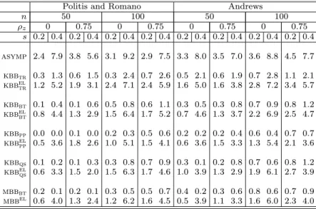
4

Table 1 reports the empirical rejection rates of the Hansen (1982)'s J test. The results obtained

reveal that the J test based on asymptotic critical values are slightly undersized for s = 0:2 and they

become to some extent oversized for s = 0:4: Note that in the latter case the rejection frequencies do

not get closer to the nominal size when the sample size increases from 50 to 100.

5

_{The tests based on}

standard KBB and MBB critical values are considerably undersized. The tests based on the empirical

likelihood versions of the bootstrap methods although are undersized for s = 0:2; yield empirical rejection

rates closer to the nominal size for s = 0:4:

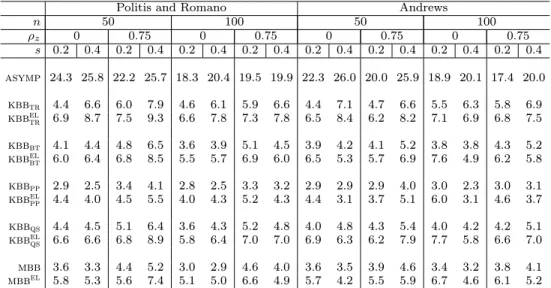
Table 2 presents the results on the t-tests for the hypothesis H

0

:

0

= 3. The empirical rejection

rates of the t-tests based on the asymptotic critical values are considerably larger than the nominal

rate. On the other hand, the performance of the t-tests based on the critical values obtained with MBB

and KBB are noticeably better than those based on the asymptotic critical values. However, the t-tests

based on the taper of Paparoditis and Politis (2000) are undersized. The empirical-likelihood versions

of these t-tests, in general are slightly oversized, apart from the case in which the kernel version of the

taper of Paparoditis and Politis (2001).

Overall the results obtained with both methods to compute the automatic bandwidth are very similar

4_{The results on 1% and 10% nominal level were also computed and are available upon request.}

5_{Note that these results are di erent to those reported by Hall and Horowitz (1995), specially in the case s = 0:4,}

Table 1: Empirical rejection rates of the J-tests with asymptotic and bootstrap critical values at 5%

level

Politis and Romano Andrews

n 50 100 50 100 z 0 0:75 0 0:75 0 0:75 0 0:75 s 0:2 0:4 0:2 0:4 0:2 0:4 0:2 0:4 0:2 0:4 0:2 0:4 0:2 0:4 0:2 0:4 asymp 2:4 7:9 3:8 5:6 3:1 9:2 2:9 7:5 3:3 8:0 3:5 7:0 3:6 8:8 4:5 7:7 kbbtr 0:3 1:3 0:6 1:5 0:3 2:4 0:7 2:6 0:5 2:1 0:6 1:9 0:7 2:8 1:1 2:1 kbbel tr 1:2 5:2 1:9 3:1 2:4 7:1 2:4 5:9 1:6 5:0 1:6 3:8 2:8 7:2 3:4 5:7 kbbbt 0:1 0:4 0:1 0:6 0:5 0:8 0:6 1:1 0:3 0:5 0:3 0:8 0:7 0:9 0:8 1:2 kbbel bt 0:8 4:4 1:3 2:9 1:5 6:4 1:7 5:2 0:7 4:6 1:3 3:7 2:2 6:9 2:5 4:7 kbbpp 0:0 0:0 0:1 0:0 0:2 0:3 0:5 0:6 0:2 0:2 0:2 0:4 0:6 0:4 0:7 0:7 kbbel pp 0:5 3:6 1:8 2:6 1:0 5:1 1:5 4:1 0:6 3:6 1:5 3:3 1:3 5:4 2:1 3:6 kbbqs 0:1 0:2 0:1 0:3 0:3 0:8 0:7 0:9 0:3 0:1 0:2 0:8 0:7 0:6 0:8 1:2 kbbel qs 0:6 3:3 1:5 2:0 1:5 6:3 1:7 4:6 1:0 3:9 1:3 2:9 1:9 6:1 2:7 3:9 mbbbt 0:2 0:1 0:2 0:1 0:3 0:5 0:5 0:7 0:4 0:2 0:3 0:6 0:8 0:6 0:7 0:9 mbbel _{0:6 4:0 1:3 2:4 1:2 6:2 1:6 4:5 0:5 3:9 1:1 3:3 1:6 6:0 2:3 4:0}

which may indicate that the proposed methods are robust to the choice of this parameter.

6

Conclusion

In this article we put forward new bootstrap methods for models de ned through moment restrictions

for time series data that build on the kernel block bootstrap method of Parente and Smith (2018a,

2018b). These methods approximate the asymptotic distributions of tests for overidentifying conditions,

parametric restrictions and additional moment restrictions. We consider methods that impose the null

hypothesis, methods that impose the maintained hypothesis and methods that do not impose any

restric-tion in the way the bootstrap samples are generated. We prove the rst-order validity of the methods

generalizing and correcting the work of Allen et al. (2011) and Bravo and Crudu (2011). A simulation

study reveals that the proposed methods perform well in practice.

Appendix: Proofs

Throughout the Appendix, C and will denote generic positive constants that may be di erent in di erent uses, and C, M, and T the Chebyshev, Markov, and triangle inequalities respectively. We use the same notation of Goncalves and White (2004). For a bootstrap statistic W_T(:; !) we write W_T(:; !) ! 0 prob P ; prob P if for any " > 0 and any

> 0, limT!1P[PT ;![jWT( ; !)j > "] > ] = 0:

A.1

Proofs of the results in subsection 2.1.1

Proof of Theorem 2.4:As Tauchen (1985) and Ruud (2000) we recast the test for H0as a test for parametric restrictions

qa

t( ; ) qt( ) and construct the moment indicators hat( ; ) (gt( )0; qta( ; )0): Under the null hypothesis = 0;

Table 2: Empirical rejection rates of the t-tests with asymptotic and bootstrap critical values at 5% level

Politis and Romano Andrews

n 50 100 50 100 z 0 0:75 0 0:75 0 0:75 0 0:75 s 0:2 0:4 0:2 0:4 0:2 0:4 0:2 0:4 0:2 0:4 0:2 0:4 0:2 0:4 0:2 0:4 asymp 24:3 25:8 22:2 25:7 18:3 20:4 19:5 19:9 22:3 26:0 20:0 25:9 18:9 20:1 17:4 20:0 kbbtr 4:4 6:6 6:0 7:9 4:6 6:1 5:9 6:6 4:4 7:1 4:7 6:6 5:5 6:3 5:8 6:9 kbbel tr 6:9 8:7 7:5 9:3 6:6 7:8 7:3 7:8 6:5 8:4 6:2 8:2 7:1 6:9 6:8 7:5 kbbbt 4:1 4:4 4:8 6:5 3:6 3:9 5:1 4:5 3:9 4:2 4:1 5:2 3:8 3:8 4:3 5:2 kbbel bt 6:0 6:4 6:8 8:5 5:5 5:7 6:9 6:0 6:5 5:3 5:7 6:9 7:6 4:9 6:2 5:8 kbbpp 2:9 2:5 3:4 4:1 2:8 2:5 3:3 3:2 2:9 2:9 2:9 4:0 3:0 2:3 3:0 3:1 kbbel pp 4:4 4:0 4:5 5:5 4:0 4:3 5:2 4:3 4:4 3:1 3:7 5:1 6:0 3:1 4:6 3:7 kbbqs 4:4 4:5 5:1 6:4 3:6 4:3 5:2 4:8 4:0 4:8 4:3 5:4 4:0 4:2 4:2 5:1 kbbel qs 6:6 6:6 6:8 8:9 5:8 6:4 7:0 7:0 6:9 6:3 6:2 7:9 7:7 5:8 6:6 7:0 mbb 3:6 3:3 4:4 5:2 3:0 2:9 4:6 4:0 3:6 3:5 3:9 4:6 3:4 3:2 3:8 4:1 mbbel _{5:8 5:3 5:6 7:4 5:1 5:0 6:6 4:9 5:7 4:2 5:5 5:9 6:7 4:6 6:1 5:2}

De ne r ( ) = (a ( )0; 0_{) and the unrestricted GMM objective function}

^

Qa( ) = ^ha( )0^ 1^ha( ): Consider the GMM estimator

^e_{= arg min} 2

^ Qa( ): As pointed out by Ruud (2000, p. 574-575) the sub-vectors of ^ are

^e _{= arg min} 2B

^

g( )0^ ^g( ); ^ = q( ^)^ ^21^111g( ^):^

We note that by Theorem 2.1 ^e ₌

0+ op(1) also as ^ = + op(1) and 11 is invertible we have by a UWL that

^ = op(1) as E(hat( 0; 0)) = 0 under the regularity conditions of the Theorem 2.1. and

p

T (^e 0) d

! N(0; ) by Theorem 2.2 as 02 int(B) and 0 2 int(R) = R where = (D0 1D).

Furthermore using the usual arguments based on rst order conditions we have p T ^ e 0 ^ = [D 0 1_D] 1_D0 1p_{T ^h}a₍ 0; 0) + op(1):

Thus by a Taylor expansion we have under H0

p T a( ^ e₎ ^ = R(•)[D 0 1_D] 1_D0 1p_{T ^h}a₍ 0; 0) + op(1) = R[D0 1D] 1D0 1pT ^ha( 0; 0) + op(1)

where • is in a line between ( ^e0_{; ^}0₎0_{and 0. Hence}

W = T a( ^e) ^ 0h ^ R( ^D0^ 1D)^ 1R^i 1 a( ^e) ^ = pT ^ha( 0; 0)0K p T ^ha( 0; 0) + op(1); as ^D = D + op(1); ^ = + op(1), ^R = R + op(1), p T ^h( 0; 0) = Op(1) and where K 1_D[D0 1_D] 1_R0 _R(D0 1_D) 1_R 1 R[D0 1_D] 1_D0 1_:

Note that K K = K and tr(K ) = s + r:Thus by Theorem 9.2.1 of Rao and Mitra(1971) It follows that W!d 2_{(r + s):}

We consider now the LM statistic