ANDERSON RAMOS PROENÇA EXPERIMENTAL CHARACTERIZATION OF

EXPERIMENTAL CHARACTERIZATION OF

VELOCITY AND ACOUSTIC FIELDS OF

SINGLE-STREAM SUBSONIC JET

UNIVERSIDADE FEDERAL DE UBERLÂNDIA

FACULDADE DE ENGENHARIA MECÂNICA

EXPERIMENTAL CHARACTERIZATION OF VELOCITY AND

ACOUSTIC FIELDS OF SINGLE-STREAM SUBSONIC JET

Dissertação apresentada ao Programa de Pós-graduação em Engenharia Mecânica da Universidade Federal de Uberlândia, como parte dos requisitos para a obtenção do título de MESTRE EM

ENGENHARIA MECÂNICA.

Área de Concentração: Transferência de Calor e Mecânica dos Fluidos.

Orientador: Prof. Dr. Odenir de Almeida Coorientador: Dr. Rod Self

UBERLÃNDIA _– MG

AGRADECIMENTOS

A conclusão desta pesquisa se deu graças ao apoio de muitas pessoas e grupos. Esperamos que o nosso reconhecimento possa extrapolar estas linhas e que cada um aqui mencionado receba um pouco do sentimento de realização emanado pelo autor, afinal, eles também são responsáveis por esta conquista.

Primeiramente, agradeço a Deus e as oportunidades que “apareceram ao acaso”. Aos meus familiares, em especial meus pais, pela educação desde os tempos de berço, e minha esposa, por me manter forte e focado nos momentos delicados durante este trabalho.

A Universidade Federal de Uberlândia e a Faculdade de Engenharia Mecânica pela oportunidade de realizar este Curso. Aos Professores que contribuíram para minha formação, especialmente ao Professor Odenir de Almeida pela orientação atenciosa e metódica e ao Professor Aristeu da Silveira Neto, pela primeira oportunidade no MFLab. Agradeço também ao Dr. Rod Self, pela confiança e paciência inigualáveis nas duas oportunidades que representam um marco divisor na minha vida profissional e pessoal. Aos amigos que foram (re)conhecidos ao longo desta vida nos colégios fundamentais, no SENAI, no ensino médio e na UFU, principalmente àqueles representantes da 80ª turma de Engenharia Mecânica. Especialmente também aos colaboradores da Organização de Jovens Espíritas (OJE) e aos trabalhadores do Centro Espírita Missão e Luz, que há mais de 4 anos possibilitam que nos meus finais de semana eu tenha oportunidade de aprender e contribuir com pessoas que diariamente enfrentam problemas escalas de grandeza maiores que o meu, exemplos de virtudes indispensáveis como humildade e resignação.

Agradeço também o Laboratório de Mecânica dos Fluidos e todos os integrantes que

conheci, especialmente o “pessoal da 303”. No nome do Dr. Jack Lawrence e do Dr. Mathieu Gruber, agradeço todos os integrantes do Fluid Dynamics and Acoustics Group, localizado no Institute of Sound and Vibration, na Universidade de Southampton, em que fui recebido de maneira singular.

A CAPES pelo apoio financeiro através da bolsa de mestrado. A Embraer pela oportunidade de participar de um projeto de pesquisa envolvendo os pontos de vista acadêmico e industrial, e pelo financiamento de viagens e conferências que acrescentaram muito neste trabalho. Ao Rolls Royce UTC pelo financiamento e acompanhamento dos experimentos realizados.

PROENÇA, A. R. Caracterização experimental do campo de velocidade e campo

acústico de um jato simples subsônico. 2013 149 f. Dissertação de Mestrado,

Universidade Federal de Uberlândia, Uberlândia.

Resumo

O objetivo deste trabalho é estudar e caracterizar aerodinamicamente um jato livre operando em regime subsônico e identificar a assinatura acústica do mesmo. Esse estudo busca analisar fundamentalmente as estruturas turbulentas e o ruído total produzido em diferentes números de Mach. Tal estudo é crucial para o entendimento desses mecanismos de geração e propagação, e encontra extrema importância para aplicações aeronáuticas, como, por exemplo, a exaustão de motores a reação (jato). A investigação é feita através da análise dos dados obtidos em experimentos utilizando tubo de pitot, anemômetro de fio-quente e ensaios acústicos. Neste trabalho também são descritos os procedimentos experimentais de cada etapa de análise, bem como as características dos laboratórios utilizados para o estudo do ruído de jato. Com os dados provenientes das medições com tubo de pitot são estudados os perfis de velocidade média. As propriedades médias também são analisadas com o sistema de anemometria, que ainda é utilizado para estudo da intensidade turbulenta em onze linhas axiais, variando da linha de centro até a borda do bocal (lipline). Estes resultados são comparados com a literatura e é constatada a acurácia dos anemômetros de fio-quente para intensidades turbulentas menores que 15%. Os dados aerodinâmicos mencionados são obtidos para números de Mach 0,25, 0,50 e 0,75, a partir da saída do bocal até treze diâmetros na direção do jato. O estudo acústico é feito através da análise do nível de pressão sonora obtido em seis posições no campo distante, com ângulos de observação variando de 40 a 110º. Diferentes velocidades também foram analisadas, desta vez, com números de Mach de 0.18 a 1.00 com passo de 0.05. Um banco de dados com o nível de pressão sonora em função da frequência é construído a partir destas informações.

PROENÇA, A. R. Experimetal characterization of velocity and acoustic fields of

single-stream subsonic jet. 2013 149 p. M. Sc. Thesis, Universidade Federal de Uberlândia,

Uberlândia.

Abstract

The purpose of this work is to study and characterize aerodynamically a free jet operating at subsonic regime and identify its acoustic signature. This study aims to analyze fundamentally the turbulent structures and the total noise produced at different Mach numbers. This kind of research is crucial to the understanding of these mechanisms of noise generation and propagation, and it is extremely important for aeronautical applications, for instance, the jet engine exhaust. The research is done by analysing the data obtained in experiments using pitot tube, hot-wire anemometer and acoustic measurements. This work also describes the experimental procedures for each step of analysis, as well as the characteristics of jet noise facilities. The data from measurements with a pitot tube was used to study the mean velocity profiles. The average properties are also analyzed with an anemometry system, likewise used to study the turbulent intensity at eleven axial lines, ranging from the centerline to the edge of the nozzle (lipline). These results are compared with literature and has verified the accuracy of hot-wire anemometers for turbulent intensities lower than 15%. The aerodynamic data are obtained for Mach numbers 0.25, 0.50 and 0.75, from the nozzle exit to thirteen diameters in the direction of the jet. The acoustic study is carried out by analyzing the sound pressure level obtained at six positions in the far field, with observer angles ranging from 40 to 110º. In this campaign more velocities are studied with Mach numbers from 0.18 to 1.00 with step of 0.05 are described. A database with the sound pressure level as a function of frequency is constructed from this information.

LIST OF SYMBOLS

Roman Symbols

Ambient sound speed, m/s

Sound speed in gas, m/s

Specific heat capacity (constant pressure), J/(kgK)

Specific heat capacity (constant volume), J/(kgK)

Cross-stress tensor

Jet diameter, m

Turbulence energy spectrum

Frequency, Hz

Sound intensity, W/m

Turbulent kinetic energy, m²/s-2

Length scale, m

Leonard's stress tensor

Mach number

Jet Mach number

Ambient pressure

Dynamic pressure

Total pressure

Pressure ratio

is the viscous stress tensor.

Radial coordinate

R Gas constant, J/K

St Strouhal number,

ij

Lighthill’s stress tensor

Jet exit temperature, K

Ambient temperature, K

Temperature ratio

Jet exit velocity, m/s

Mean velocity, m/s

velocity fluctuation at a point

Radiated sound power by a monopole source

Radiated sound power by a dipole source

Radiated sound power by a quadrupole source

Axial coordinate

Greek Symbols

λ Dissipation length scale (Taylor macroscale)

Wavelength

Kronecker delta function

ε Turbulent dissipation rate

η Kolmogorov length scale

θ Observer angle, °

Kinematic viscosity, m²/s

ρ Fluid density, kg/m³

Fluid density at rest, kg/m³

Thermal conductivity, W/(mK)

CONTENTS

1 INTRODUCTION ___________________________________________________ 3

1.1 General context ___________________________________________________ 3

1.2 Noise mitigation programs and noise certification ______________________ 6

1.3 Sources of aircraft noise __________________________________________ 10

1.4 Jet engines ______________________________________________________ 12

1.5 Ways to study the problem ________________________________________ 15

1.6 Projects involved _________________________________________________ 16

1.7 Objectives and author’s contribution ________________________________ 17

1.8 Thesis outline ___________________________________________________ 19

2 AERODYNAMICS AND ACOUSTICS THEORY OF SUBSONIC JETS________ 21

2.1 Jet aerodynamics ___________________________________________________ 21 2.1.1 Basic physics of single jets _________________________________________________ 26

2.2 Jet turbulence ______________________________________________________ 30 2.2.1 General concepts of turbulent flows __________________________________________ 30 2.2.2 The turbulence spectrum ___________________________________________________ 32 2.2.3 The circular jet structures __________________________________________________ 34 2.2.4 Basic governing equations _________________________________________________ 36

2.3 Jet aeroacoustics ___________________________________________________ 38 2.3.1 Radiation of sound _______________________________________________________ 39 2.3.2 Directional sound pattern in jets _____________________________________________ 41

2.3.3 Lighthill’s acoustic analogy _________________________________________________ 43

3 LITERATURE REVIEW_____________________________________________ 46

3.1 Experimental research in single jets ___________________________________ 46 3.2 Jet noise facilities __________________________________________________ 51 3.2.1 General features _________________________________________________________ 51 3.2.2 Test facilities by description ________________________________________________ 55

4 METHODOLOGY _________________________________________________ 67

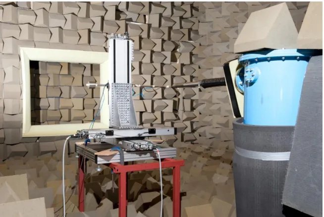
4.1 Doak Lab __________________________________________________________ 67 4.1.1 Flow control and ambient condition measurements ______________________________ 70 4.1.2 Data acquisition system ___________________________________________________ 73

4.2 Aerodynamic equipment _____________________________________________ 75 4.2.1 Pitot Tube ______________________________________________________________ 75 4.2.2 Hot-wire anemometer _____________________________________________________ 76 4.2.3 Traverse system _________________________________________________________ 78 4.2.4 Sensors calibration _______________________________________________________ 79

4.3.1 Microphones ____________________________________________________________ 80 4.3.2 Preamplifiers ____________________________________________________________ 81 4.3.3 Amplifiers _______________________________________________________________ 82 4.4.4 Calibration procedure _____________________________________________________ 83

4.4 Experimental procedure _____________________________________________ 83 4.5 Post-processing ____________________________________________________ 88

5 EXPERIMENTAL RESULTS _________________________________________ 90

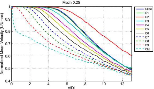
5.1 Aerodynamics results _______________________________________________ 90 5.1.1 Mean velocity profiles _____________________________________________________ 90 5.1.2 Velocity fluctuation ______________________________________________________ 107 5.1.3 Power spectral density ___________________________________________________ 113

5.2 Acoustic results ___________________________________________________ 115 5.2.1 Sound Pressure Level vs velocity ___________________________________________ 115 5.2.2 Sound Pressure Level vs Observer angle _____________________________________ 117

6 CONCLUSION __________________________________________________ 121

6.1 Concluding remarks _______________________________________________ 122 6.2 Future works______________________________________________________ 123

REFERENCES ____________________________________________________ 124

APPENDIX I ______________________________________________________ 130

APPENDIX II _____________________________________________________ 134

CHAPTER I

INTRODUCTION

The word “Aeroacoustics” refers to the study of sound produced by flows and this

chapter gives one general vision about the principal issue around this subject: aircraft noise. It is explained why aircraft noise is a question related to the daily lives of many people, which requires much effort from companies and the scientific community. It discuss as some programs that are used to deal with the aircraft noise and the sources of noise coming from different aircraft components and phases of flight. Some solutions are shown and as well as brief words about the noise related to the jet engine, the main subject of this work. Finally, a summary about the thesis’ chapters contents concludes the introduction.

1.1 General context

The modes of transport or ways of travel were always guided among the topics of greatest interest of humanity. Traversing quickly over the centuries, there has been the development of ships, trains, cars and aircraft, beyond a diverse range of modifications and

innovations. The concept of “long trips” modifies itself, where what was long becomes short even though the physical distance remains unchanged. Safety, comfort, speed and also leisure items are increasingly exploited in transportation.

in the early 1960s (Smith, 1989). The aircraft noise is the noise pollution produced by any aircraft or its components during a flight.

In comparison with the older airplanes, those of today are much quieter than 20 years ago and will be replaced by even quieter aircraft in the future (Lee and Edmonds, 2011). The modern high bypass turbofan engines are quieter than the turbojets and low bypass used before. Nevertheless, from another point of view, the number of flights is increasing and the local noise limits are more restrictive. The aircraft became 75% less noisier over the last 30 years, however the air traffic is growing and citizens are still exposed to high noise levels. To guarantee airports working at permitted noise levels, noise monitoring systems have been installed. The Fig. 1.1 shows information about Heathrow Airport to illustrate the case. The graph is about the population and the total area within the 57 dBA from 1988 to 2011. Additionally, movements per annum in that airport are also explored. The data proof that the number of people affected had been decreasing, however last years the trend is more to be stabilized than decrease.

Figure 1.1 – Heathrow traffic and noise contour area/population trend (1988 – 2011) –

Source: ERCD Report 1201 – Noise Exposure Contours for Heathrow Airport 2011

long been one of the most significant challenges facing airport operators and their neighbours.

The generation of noise happens whenever the passage of air over the aircraft structure or through its power-plant causes fluctuating pressure disturbances. To have the flight conditions efficiently is extremely necessary maintain these air and gas flows controlled efficiently. Thus, there are many contributors for noise to be produced.

Figure 1.2 shows the trend of noise exposure to aircraft noise (global trend), which plots the population in millions exposed to the aircraft noise for 55, 60 and 65 dB along the years 2000 to 2025.

Figure 1.2 – Trend of noise exposure to aircraft noise. Source: 7th _{USA/Europe Air Traffic}

Management R&D Seminar, Barcelona 2007, “Trends in Global noise and emissions from commercial aviation for 2000 through 2025”.

This unit takes into account the sound energy received by a listener, the ear’s response, the

added annoyance of pure tones in the noise and the duration of the noise. The studies are often related to explain how and how much the body respond to aircraft noise in terms of health, sleep, welfare and performance.

1.2 Noise mitigation programs and noise certification

With the new rules about the noise limits which some airports adopted in the past, many aircraft could see their operation days counted. The development of better technologies in terms of aircraft noise was inevitable, but the old aircraft ones had to find alternative solutions in order to keep working. It was not rarity to those extremely noisy aircraft flight lightweight to increase their climb performance until reach one airport less sensitive to the noise limits and then take on the fuel needed to arrive at the final destination (Smith, 1989). Although it could solve the problem with some airports, it increased the fuel and time wasted during one travel.

After recognized as a real issue, the aircraft noise was responsible for the creation of both local and international authorities, as well as the modification of some aircraft

organizations to include the subject “Noise” in their programmes. The “noise certification” is

the process which the aircraft manufacturers have to demonstrate that their product meets basic noise and safety standards.

Figure 1.3 – Congonhas Airport

The International Civil Aviation Organization – ICAO – introduced noise certifications which made the premature demise of many models. ICAO is a specialized agency of the United Nations, created in 1944 to promote the safe and methodical development of international civil aviation throughout the world. Both the EU and the UK have adopted

ICAO’s recommended “Balanced Approach to Airport Noise Management”. This Balanced

Approach consists of four main elements: noise at source, operating procedures, land use planning and operational restrictions. In the United States of America, since aviation is a public issue around late 1960s, there are legislations around the aircraft noise controls.

Figure 1.4 – Trajectory and certification locations (Hupe, 2008).

Other important organization is the Federal Aviation Administration, or FAA, created in the United States of America. Aircraft were divided into “Stages” according to weight, number of engines and passenger capacity. Aircraft noise levels are certified as Stages 2, 3 and 4. The Stage 1 aircraft are the ones which never had been tested and certified before and it is expected them to be the loudest. Stage 2 aircraft are the second noisiest, and so on. In 1990, during a congress in the USA, the Airport Noise and Capacity Act agreed to the phasing out Stage 1 and Stage 2 aircraft, but just to aircraft weighing more than 75000 pounds (or around 34 tonnes). A group of airport operators, mainly in Ohio, New York and New Jersey States are trying to change that, since the small aircraft at first Stages has caused an annoying noise. The group says the real action can only come from trying to reduce noise at its source. The Stage 4 was stated in 2005, when the FAA adopted a new noise standard for subsonic jet aircraft and subsonic transport category large aircrafts. Thus, the new aircraft design must incorporate the latest available noise reduction technology after 1st _{January, 2006. The USA Congress has also authorized the FAA to devise programs to}

insulate houses near airports.

international measure, represents equivalent continuous noise level) and Lden (split the measures in Lday, Levening, Lnight, each one related to specific hours during the day). The UK Government says people start to become significantly annoyed by aircraft noise by 57 dB LAeq. Reports were developed and a study about the aircraft noise close to the airport and its distribution was carried out. A comparison along the years show that in 1980, 2 million people had been living in a region with 57 dB LAeq contour and it was reduced to around 252,000 in 2010, despite the fact the runway had increased almost twice. Fig. 1.5 shows one example of the LAeq contour comparison between the years 2010 and 2011. As well as the FAA provide in United States, the houses close to Heathrow airport has received noise insulation and vortex protection schemes (Lee and Edmonds, 2011).

Figure 1.5 – Heathrow 2010 and 2011 LAeq contours (Lee and Edmonds, 2011).

Many airports also have a night flying restrictions like Congonhas Airport in Brazil and

London’s airports Heathrow, Gatwick and Stansted. The purpose is to reduce noise exposure at night, when the background noise is lower than during the day and the neighbours are sleeping, increasing the sensibility to noise. Thus, the noise events are perceived to be louder. The FAA adds a 10 dB penalty to aircraft operations conducted between 10:00 p.m. and 7 a.m.

noise at its source, land-use planning management, operational measures and operational restrictions. They can be looked individually, however is common to work with them integrated. The development of each section depends on pace of technological improvements, or research programmes, and usually involves high costs/time (Hupe, 2008).

The European “Visions 2020” is proposing to reduce the noise impact by one half

relative to 2000 technology and the USA Noise Reduction Goals, to reduce perceived noise impact by ¾ within 25 years (from 1997) (Dobrzynski, 2008). Recently, a new approach was inserted in this context, called Flightpath 2050 (European Commission, 2011). This program was produced by the aviation community focused on two main challenges: meeting the needs of the European citizens and the market, as well as maintaining global leadership. One of the environment goals is to reduce the perceived noise emission of flying aircraft by 65%, moreover reduction in CO2 and NOx emissions.

Also, there are many examples of projects between companies and universities. A huge integrated aircraft noise project, the SAX-40, a silent aircraft, is one of the most well-knowns. The goal is to develop a conceptual design for an aircraft whose noise would be almost imperceptible outside the perimeter of a daytime urban airport. The timeframe is about 2030 and many technical challenges have to be overcome until there. They desire to reduce noise but also fuel burn by eliminating level segments, keeping aircraft higher and at lower thrust levels for longer than traditional landing approaches. The project is developed by two universities, Cambridge University and Massachusetts Institute of Technology, as well as aerospace partners, as industry, airline and airport operators. That is just a brief sample to show how many companies and universities are working hard in order to develop new tools and solutions to this issue and research groups are usually divided into the subjects involved.

1.3 Sources of aircraft noise

Figure 1.6 – Aircraft and noise sources

Many efforts have been made to understand the noise produced by engines and their sections separately. The turbines and other mechanical parts are the mainly responsible for the noise produced during the take-off and climb and in a general point of view the major sources of aircraft noise. During the approach, the engine noise is also considerable. However, due the advances in engine noise reduction, the airframe is noisier during this phase. The engine noise also can be divided into two general categories: internally generated noise or turbomachinery noise and externally generated noise or jet noise. The turbomachinery noise can also be divided from its components, comprised of fan noise, compressor noise, combustion or core noise and turbine noise. Although high bypass-ratio turbofans have considerable fan noise, the jet noise is responsible for the majority of engine noise (Almeida, 2009). This subject is extremely important and is the main motivation of this work.

Figure 1.7 brings information about the noise during the take-off and approach according to the sources related to the airframe and engine.

Figure 1.7 – Noise component breakdown at take-off and approach (Almeida, 2009)

The aircraft systems like the cockpit, cabin pressurization conditioning systems, Auxiliary Power Unit (APU) and others also increase the total noise, although their noise components are not too much expressive as the ones from the others parts of the aircraft such as stated before.

1.4 Jet engines

reduction in the first 20 years and a new rate of reduction really small in the 30 years after. With larger aircraft and higher jet velocities required in this second range, to reduce the noise of the engines the challenge had been also increased.

Figure 1.8 – Progress in aircraft noise reduction from 1955 to 2005 (Viswanathan, 2008).

The jet engines are present in most of passenger and military aircraft nowadays. They can be classified according to the type of compressor (centrifugal, axial and centrifugal-axial flow) and also the path the air takes through the engine and how power is produced.

Taking the second definition, the turbojet engine is the simplest of all jet engines. It is composed by a compressor which passes air at a high speed ratio, a combustion chamber which contains the fuel inlet and igniter, turbine section which accelerated exhaust gases providing thrust and the exhaust where the jet is discharged. All of the propulsive force derived from exhaust gas and the turbulent mixing of this exit jet within the ambient is considered the main mechanism for jet noise. Today these engines are mostly used in military aviation.

often used in small aircraft and agricultural applications, once they are suitable to perform well at slow airspeeds and fuel efficiency.

The turbofan engines were designed to merge the best features of the turbojet and turboprop and they are largely used today. There is an additional thrust to diverting a secondary airflow around the combustion chamber. The air in the first stage enters the compressor section as in the turbojet. The secondary stage bypass the engine core and exiting at increased pressure and velocity through the fan exhaust. It also can leave the nozzle separately or mixed from the primary or potential engine air. The jet noise benefits arise from the fact that the turbofan jet exhaust velocities are lower than those of a turbojet, since the jet temperature is lower due the mixing between hot flow (potential core) and cool flow (secondary core) and the additional energy added by the extra turbine stages. For example, the early turbojets exhaust velocities were of order 650 m/s and modern turbofans have velocities lower than 450 m/s in the potential core and less than 300 m/s in the cold stream. About 75% of the propulsion comes from the fan and 25% comes from exhaust gas. Today the most used engines are the high bypass ratio turbofan engines. It was primarily developed for fuel saving but it also brought significant reduction in jet noise (Almeida, 2009).

The term “jet noise” is usually taken to mean the noise of jet-powered aircraft. However, strictly speaking, it is about only those sources associated with the mixing process between the exhaust flow of the engine and the atmosphere, as was said before during the division in jet and turbomachinery noise. This mixing noise is the only component generated during subsonic operations. In super critical jet there is also a secondary noise source which appears from shock-waves.

1.5 Ways to study the problem

Likewise many engineering problems, the aerodynamic and acoustics jet surveys can follow three paths: analytical, numerical and experimental investigations.

When the Reynolds number is high or, in other words, when the nonlinearities due to the inertial terms in the equation of motion are much larger than the viscous terms, to solve the governing equations become even more difficult. In fact a good mathematical model to depict the real physics or as close to real as possible solved analytically generally requires too much effort. Nevertheless, first principles methodologies such as Lighthill equations published in 1952 are well known. That paper is considered a birth of the research area

“Aeroacoustics”. The motivation was to predict the sound produced by a free jet, and the new approach was called by himself an “analogy”, providing a formal definition of the acoustical field in the presence of a flow. The sound production represents a tiny fraction of the energy in the flow and the direct prediction of sound generation is very difficult, so this acoustical filed is an extrapolation of an ideal reference flow, where the difference between both is identified as a source of sound. Another important point to highlight in this work is the proportion between the sound intensity produced by turbulence and the local volume over which the turbulent stresses are correlated. Thus, for any methodology it is clear that study the fluid dynamics related to the jet is extremely important to understanding jet noise (Schram, 2003; Tam, 1998; Rienstra and Hirschberg, 2011).

There are many techniques available considering different mathematical and numerical approaches. Semi-empirical methods and computational fluid dynamics (CFD) coupled with computational aeroacoustics (CAA) comprehend other possibilities. While

space than the corresponding velocity field (where is located the Lighthill’s sound sources)

this theory is more convenient for low Mach numbers and isothermal flows.

Many different numerical methods appear each year including new methodologies

and modifications of the “old” ones. The physics of jet is always involved with the acoustic

issue, thus a numerical model is composed by the transport phenomena equations, turbulence models, discretization methods and so on. Direct Numerical Simulations (DNS) are being made as well as Large Eddy Simulations (LES) and Reynolds Average Numerical

Simulations (RANS), but when solving some real configuration in an “industrial time”, the

Reynolds numbers used in reliable simulations are still below the range of the practical applications. The advent of new technologies in computer field has helped to improve these methodologies but it has yet to be improved in order to obtain accurate results with less computational costs.

Probably the most established way of investigating a subject that we turn our attention is to perform controlled experiments. In this case, real scale experiments often become prohibited since the costs involved are too high. In a world where things change so frequently and new products are expected, experiments with such costs are not interesting to manufacturers. Scale experiments or reduced models are very important in this context and the knowledge about the data and its extrapolations are really useful. By considering semi-empirical or semi-empirical methods, it can be said that these methods are fast, reliable and have a long application in industry. However, one of the greatest problems in these methods is the restriction or applied considerations used to derivate them and also the envelope of operating conditions to be applied. As tailored tools for some specific jet noise predictions, many times they are restrictive to certain geometries, velocities, temperature and pressure ranges. Nevertheless, it is also observed that companies and organizations are interested in predicting the noise from jets using methods related to particular cases, and, sometimes, for just only one family of aeronautical engines. A deeper approach will be made in later chapters about the test facilities, equipment, sensors and the ways to acquire data from jet experiments.

1.6 Projects involved

Part of the present work was developed along with Embraer S. A., a Brazilian aircraft

manufacturer, by means of two projects: “Silent Aircraft: An Aeroacoustics Survey” and

first one was also funded by the São Paulo Research Foundation (FAPESP), while the second phase was sponsored by Funding of Studies and Projects (FINEP). Those projects are divided in subgroups according to the subject, which this work is into the Jet Noise group. The integrated project is compound by some Brazilian’s universities, among them the

Federal University of Uberlândia.

This work is also part of a cooperation project between the University of Uberlandia and the University of Southampton, specifically the Institute of Sound and Vibration Research. The jet aerodynamic and acoustic results were provided in the ISVR’s laboratory

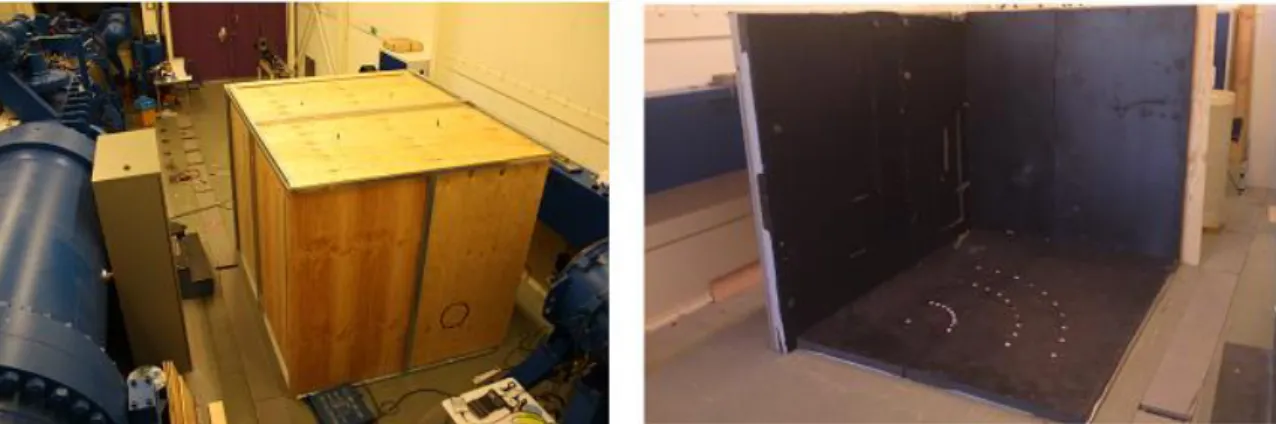
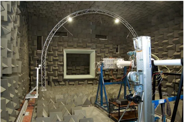
called DOAK Lab. The test matrix was built up in beginning of August, 2011, and the measurements were made with the supervision of the Fluid Dynamic and Acoustics Group –

FDAG, especially Dr. Rod Self. The laboratory in question is an anechoic chamber built for subsonic and supersonic acoustic measurements. This work also was done to extend the applications of the DOAK Lab to aerodynamic measurements, what will be shown in another chapter.

1.7 _{Objectives and author’s contribution}

The general purpose of this work is to study and characterize aerodynamically a free jet operating at subsonic regime and identify its acoustic signature. The survey is divided in two sections: aerodynamic results for a free, single, subsonic and cold jet at Mach numbers of 0.25, 0.5 and 0.75 and acoustic results to the same kind of flow at Mach numbers 0.15 to 1.00, through a step of 0.05. In the aerodynamic study, mapping the jet using pitot tube and comparing the results with the hot-wire anemometer were done in order to plot the mean and fluctuating profile velocities and test the hot-wire resistance at high flows. There is a lack in results of hot-wire anemometry of high frequency response at high velocities (e.g., Mach 0.75), and the present work bring considerable information for different jet velocities and a wide domain around the jet. The acoustics results take place in the database context as well as a basic theory directed for a wide velocity range.

Engineering was started at the University in 2010 and has recently arrived to the application courses, including the subject of Aeroacoustics. Therefore, one of the goals is to perform a fundamental analysis over the subsonic jet looking at a complete mapping of the jets region at different velocities. This review is done through literature comparisons and correlations among the aerodynamics and acoustics data shown.

The results presented herein are not restricted only to the experimental front, but also to the surveys with semi-empirical methods and even numerical methods which need some input parameters or validation. While the Group has been developing numerical methods at the Fluid Mechanics Laboratory (MFLab), an expansion to build an anechoic chamber is desired for a near future, where the experience acquired in this work will be applied. The present work dedicated one sub-section to discuss the mainly parameters of an anechoic chamber.

As stated before, some aims coming from involved projects. Currently, an anechoic

chamber has been built at Federal University of Santa Catarina as part of EMBRAER’s

Project. The familiarity about basic equipment, tools, sensor, air supply and data acquisition achieved in this work is also a support to that Project. The cooperation with the ISVR during the experiments aims the acquisition of knowledge about jets and enlarges the laboratory to reliable aerodynamic measurements.

The points described can be summarized as:

 This work is an “initial guide” in terms of basic knowledge about the topic to students who are starting in this subject and aim to join the Aeroacoustics Research Group at the Federal University of Uberlandia working within the experimental area.

 Mapping of the mean velocity along axial and radial lines from the jet using pitot tube and hot-wire anemometer. Turbulence intensities or fluctuating velocities along axial and radial lines from the jet using hot-wire anemometer are also studied.

 Noise of a free jet in comparison with the aerodynamic results, since the understanding of jet noise is tied to the understanding of turbulence in jet flows. Also, a review of the most important terms in jet aeroacoustic, including the basic theory involved, instruments used during the measurements, far-field results for different observer angles and velocities.

 Some modifications were made in the DOAK Laboratory to enable aerodynamic measurements, what revealed some issues to improve the system and the results shown that it was achieved.

 Understanding about measurements, equipment, sensors and test facilities of jet aerodynamic and jet noise measurements.

1.8 Thesis outline

This work was developed at the Federal University of Uberlandia (UFU) in cooperation with the Institute of Sound and Vibration Research (ISVR) located at University of Southampton. It was supported by the Rolls Royce UTC in Gas Turbine Noise, the

Brazilian technological development project called “Aeronave Silenciosa”, and the UNIEMP Institute during the first experiments (2011) and CAPES during the properly MSc period (2012 – 2013). The experimental activities were conducted at ISVR in the period from August to December in 2011 and March to May in 2013. From January in 2012 until here the activities were conducted at UFU.

The thesis is composed of six chapters.

Chapter 1 gives an introduction about the main subject of this work. A general context is presented going from the most general observation until the subject of this work. It is also exposed about some programs to reduce aircraft noise and noise certifications. The sources of aircraft noise are soon mentioned and a general vision to the jet engines and jet noise is given. Lastly, the ways to explore the problem and the main objectives were shown.

The basic theory related to aerodynamic and acoustics of free single jets is given in Chapter 2. This chapter composes an important item for those who during the regular graduation course did not have the opportunity to further study the jets physics.

The bibliography review is presented in Chapter 3. The focus of this chapter is on the modern experimental works around jets using pitot tube, hot-wire anemometry and far-field and near-field acoustics. Also, some jet rigs around the world are brief discussed.

Chapter 4 shows the methodologies taken in this work. The rig is described as well as equipment, sensors, data acquisition systems and post-processing scripts. The experimental procedure is also evidenced. The tests matrix used during the experiments and some sketches for the principal contents and configurations are presented.

measurements. Some velocities profiles are also showed. For the acoustical results, the spectrum of sound pressure level graphs for the condition studied taken place.

The conclusion of this work is presented in Chapter 6, general observations and comments are made, which is a summary along the main results, principal issues which had to be solved along the whole work, and the suggestions to future works.

CHAPTER II

AERODYNAMICS AND ACOUSTICS THEORY OF SUBSONIC JETS

“Fluid mechanics is the study of fluids either in motion (fluid dynamics) or at rest (fluid

statics) and the subsequent effects of the fluid upon the boundaries, which may be either

solid surfaces or interfaces with other fluids” (White, 1991). That is important to contextualise the sections presented in this work: although the main aim is to predict and hereafter control

the noise produced by flows, it is indispensable to study the jet’s physics theory, once the

structures formed along this flows are closely associated with noise production. Therefore, the jet noise topic is a multidisciplinary subject, where the understanding of fluid mechanics is imperative to aeroacoustics.

This chapter is a brief summary of the aerodynamic and acoustic theory related to jet

flows. First of all, a general overview of the jet’s physics of single flows is given. This section

is divided mainly in aerodynamic and turbulence parameters in free jets. The aim is to present the most important aspects and variables. Secondly, some remarks about the basic principles of acoustics and the Acoustic Analogy of Lighthill are presented.

2.1 Jet aerodynamics

A free jet flow occurs when a fluid is pressurized in a duct and moves out through a nozzle discharging in a quiescent medium. This particular flow can be classified according to many parameters, which the important ones are explained below.

results shown in this and most studies in the literature are conducted on circular nozzle. That is totally understandable since most of the current jet engines have a round nozzle.

(a) (b)

Figure 2.1 – (a) Rolls Royce Trent 900 engine which generates a coaxial circular jet. (b) Indy Transponder with rectangular nozzle.

(a)

(b)

Figure 2.2 – Examples of: (a) a turbojet (single jet); and (b) a turbofan (coaxial jet).

There are also cases where two or more jets are discharged not on the same axis, but in a crossflow geometry, the called cross-jets. Beyond the shock between jets, there are many examples of jet interactions. Actually, along practical applications in aircraft, the jet is frequently interacting with other parts, such as wing and fuselage. In a more general point of view, many studies are interested in the interaction between a jet and a surface, forming the class of installed jets. Whilst the study of free jets has had an important role in the development of engines and other machines along the years, the research associated with installed jet has been the interest of aerodynamic and acoustic measurements.

Figure 2.4 – Simulation of exhaust nozzle under installed configuration (Argonne National Laboratory).

Temperature involved in the process is another parameter which can change the problem. An isothermal jet is represented where there is no difference (or it is negligible) between the temperature of the jet and the temperature of the ambient. When the jet is heated in relation to the medium, some particularities are found. In the case of more than one jet, coaxial or cross-flow jets, for example, there is a temperature ratio between the jets from different sources, which also changes the properties of the jets in comparison with the isothermal ones.

terms, subsonic flows are the ones which the mean velocity is under the speed of sound in that ambient, whilst supersonic flows the velocity is higher than the speed of sound (higher than Mach 1). The physics related to subsonic and supersonic flows are substantially different, since the latter has the formation of shock waves which in turn directly the profile of the aerodynamic properties as well as the noise sources. Other classifications are given, such as transonic (around Mach 1) and hypersonic (Mach number higher than 5). In fluid mechanics, the Mach number is also used for other classifications: the incompressible and compressible flows. The compressibility effects are typically considered significant for Mach number higher than 0.3 or very large pressure changes in the flow. It means that for low velocities the density can be considered constant, which simplifies the governing equations, as shown in the next section. However, the jet flow applications in aeronautical devices usually exceed this Mach condition.

(a)

(b)

Situating the present work, the jet studied here is classified as a free, rounded, single, cold, subsonic, compressible jet.

2.1.1 Basic physics of single jets

According to Abramovich, “jet” is a special fluid motion where tangential separation

surfaces are evidenced. Velocity, temperature and specie concentration are some flow parameters that describes the tangential separation. Other important point related to the physical properties is the static pressure distribution along the different layers: it remains continuous (Abramovich, 1938).

Figure 2.6 – Diagram of a single jet (Abramovich, 1938).

With the end of the potential core, after four or five diameters downstream the exit jet, a transitional region arises. In this region, the uniform growth of mixing layer ceases. Its length is again four diameters and in the end of this region a self-preserving flow takes place, originating the final region called the fully developed. Therefore, the first two regions comprise the developing portion of the jet, and the mean velocity profile becomes self-similar after that. This region seems to grow from an apparent origin, as can be seen in the Fig. 2.6. Whilst the velocity profile has the same momentum, the mass rate does not remain constant. The fluid is fed back by the ambient in a process known as “entrainment”. Entrainment is the

movement of one fluid by another, which is responsible for increase the mass flow along the jet axis (Souza, 2005).

Figure 2.7 – Entrainment by an axisymmetric turbulent water jet (Van Dyke, 1982)

Besides the three regions of a single rounded jet are well established, different nomenclatures are used, for example, the near field, the intermediate field and the far field, corresponding to the initial, transitional and fully developed regions (Fellouaha and Pollard, 2009). There is no consensus about the length of each region as well, although usually it is not a substantially discrepancy.

In few words, increasing the axial distance, the jet decays and spreads. The laminar interface becomes unstable and the entire jet becomes turbulent downstream of the nozzle.

surfaces generate eddies both along and across the flow (Abramovich, 1938). More details about these structures are given in the next section.

The flow is statistically stationary and axisymmetric, which means the statistics depends on the axial and radial coordinates, but not circumferential coordinate θ. The

longitudinal velocity is some orders of magnitude higher than the transverse velocity components. For this reason, commonly velocity profile graphs and other properties are mainly governed by the jet axis component. Moreover, a fully turbulent jet discharging into ambient fluid has a mean axial velocity distribution almost independent of Reynolds number.

In order to describe the mean velocity profiles of a steady jet, a well-established method makes use of three graphs, illustrating the mean velocity profile, ⁄ , as a function

of radius , the mean centreline velocity, ⁄ , as a function of axial location x/d and

the jet half radius as a function of axial location, where is the jet mean

centreline velocity, is the radius at which the velocity is half the centreline velocity and

is the jet exit diameter (Harch and Bremhorst, 1977). Some examples are shown in the Fig. 2.8.

(a) (b)

The spreading of the mixing layer is another important characteristic of the jet flow. According to Lilley (1958), this linear spreading of the jet is consistent with the existence of large eddies, randomly distributed, which are in a form of energy equilibrium. These eddies are centered on average at the position of maximum shear.

Figure 2.9 – Mixing layer region by Almeida (2009)

The variation of the mean velocity profile and the mean square turbulence velocity across the mixing layer are shown in the next figure. It can be seen that most of the turbulent energy is confined to a fairly narrow region at the centre of the mixing layer. What has been identified by measurements is that the peak turbulence intensity occurs on the centreline of the mixing layer (Goldstein, 1976).

Figure 2.10 – Mixing layer velocity distribution (Almeida, 2009).

2.2 Jet turbulence

One of the most challenging problems of engineering and physics nowadays is a phenomenon very present in our daily routine: the turbulence in the fluids. Despite getting along with the observation of turbulence from many centuries through simple qualitative representations, the physics of this type of flow is intriguing and there is still much to learn, but the complexity is such that it has been named some researchers as the 'last of the classic problems' in open. Current studies of turbulent jet flows have been stimulated by the aircraft noise problem.

Although the laminar flow has their physics well-known and modeled mathematically, the transitional condition and fully developed turbulence is still an open field. The phenomenon of transition occurs when the laminar fluid becomes unstable with the existence of inertial forces and / or gradient of potential energy large enough to overcome the flow resistance to keep it laminar. Some factors that influence this process are known: existing level of disturbance, surface roughness before the exit nozzle, pressure gradient, compressibility effects, heat transfer and density stratification, among others. As previously mentioned, jets are transitioning flows already in the region close to the nozzle and from low velocities, becoming turbulent fully developed some diameters after the exit.

The jet in its most basic form is a type of free shear flow, i.e., it does not have submerged bodies within their domain nor some kind of solid limit on its borders. In free shear flows, the source of instabilities is connected to an inflectional velocity field. Before move along in jet turbulence, next item describes some characteristics of turbulent flows with emphasis in jet flows.

2.2.1 General concepts of turbulent flows

Turbulent flows have fluctuation of pressure and of velocity superimposed on the main flow. Generally, turbulence is a dynamic system in which the number of degrees of

freedom is “high enough” and its general concept helps in understanding the nature of the

flow jet type. Lesieur (1997) cites three fundamental characteristics for the flow to be turbulent: the flow needs to be unpredictable in the sense that small uncertainties will amplify nonlinearly,it must necessarily increase the rate of mixing of properties and it must have an extensive range of spatial wavelengths. A jet has no trouble filling these three points. Other features necessary for the onset of turbulence and its relation to the flow here studied are mentioned below (Silveira Neto, 2002).

Irregularity and instability: In the sense that a purely deterministic analysis is

was considered to be purely random. Nowadays a plausible solution presented is considered part of the scales that comprise the turbulence as deterministic (large structures) and other random (small structures). If the structure has a longer life than their time of rotation characteristic, for example, it may be considered statistically consistent. The fluctuations are time and space-dependent.

High diffusivity: Although considerations taken as inviscid fluid, the small scales are

transformed into heat by viscosity. Fluctuations generating high gradients in the flow are responsible for this event. This feature has an important practical application, since the properties mixing process is greatly accelerated, which is attractive for most jet applications.

The Reynolds number characteristic must exceed unity. Thus, the inertial forces

overcome diffusive or viscous forces. The nonlinearities that amplify the disturbances, causing instabilities, are not contained in the term inertial. Jets where the working fluid has low kinematic viscosity such as air, typically always have high Reynolds numbers.

Dimensionality and rotatability: The development of vortices and three-dimensional

structures in turbulent flows is uncontrollable. Even if a region would be irrotational, next to it there must be structures in rotation. The interaction between the vortices formed produces the effects of stretching and tilting them. Associating these movements to the velocity field, there is the appearance of components in the three orthogonal directions. The behavior of large and small structures that appear in this process occurs differently: the first line up preferentially to the main flow while the latter are well distributed, not by adopting a preferred alignment.

Process dissipative: Viscosity generates shear deformations which increase the

internal energy of the fluid. Thus, the turbulence needs a continuous supply of energy to overcome this viscous loss. Without the energy increment, turbulence decays. If the medium is non-dissipative, such as atmospheric gravitational waves and random sound waves, there is no turbulence. In the case of a jet it is important to understand the process of formation and energy transfer between the structures.

Continuous medium: Relating the smallest scales of turbulence with molecular

scale, it is clear that the smallest structures are large enough to apply the continuum hypothesis. The Navier-Stokes equations can be used to govern the fluid motion (with a limit of Mach number equal to 15, which scales no longer satisfy the molecular mean free path).

Multiplicity of scales: Necessarily, the spectrum involved in this kind of

phenomenon is continuous and wide.

of a jet relative to its mean time. Note also that the phenomenon is far from being regular and the existence of various scales.

Figure 2.11 – Mean velocity and velocity fluctuation measured during 0.3 seconds in a centreline of a low velocity jet.

2.2.2 The turbulence spectrum

As previously mentioned, a characteristic of turbulence is the existence of various length scales ranging from the domain size to the dimensions of the smallest structures, known as the Kolmogorov scale.

Following the idea of Richardson and the cascade energy transfer from larger to smaller structures (which the largest receive the highest kinetic energy of the main flow and feeds the lower scales until the viscous stress dissipate the whole energy), it is necessary for a continuous injection of energy in order to maintain the flow.

The scales of turbulence are distributed by a continuous range that extends from the lowest to the highest scale. Each of these ranges contributes an amount of turbulent kinetic

energy ‘k’, which is associated with the wave number characteristics of this scale. Therefore,

Figure 2.12 – Three regions of the energy spectrum of turbulence.

It is observed in the spectrum three distinct regions: Region I, with smaller wave numbers (large structures) and contributing the largest portion of the total energy. This is the region of energy injection. The region II, or sub-inertial range, where energy is transferred

from higher to lower scales and where there is Kolmogorov’s spectrum law, with the decay of

-5/3 and fully turbulent flow. Finally, region III, corresponding to the smaller scales, where there is dissipation of energy.

The overall turbulent kinetic energy is obtained by integrating over the space wave number:

∫ (2.1)

In that way, the kinetic energy is the sum of the three components of velocity fluctuation:

( ̅̅̅ ̅̅̅ ̅̅̅̅) ̅̅̅̅̅ (2.2)

showed in the last figure, which are: the integral length scale (l), the Taylor microscale (λ) and the Kolmogorov microscale (η). This scenario enables comparison between the energy transfer and the dissipation rate, ε. The correlation among the scales, turbulence and fluid properties are not showed in this current work, but further information on this field can be found in (Lesieur, 1997).

2.2.3 The circular jet structures

The Fig. 2.13 illustrates a turbulent circular jet and its structures. Initially, it is possible to check the appearance of the Kelvin-Helmholtz instability, which induces the formation of secondary instabilities. The interaction of primary structures with longitudinal counter-rotating filaments creates transverse oscillations, which with its amplification degenerate into turbulence. The flow conditions are very important to define the transition of flow, which normally occurs close to the nozzle exit.

Figure 2.13 – Structures in a circular subsonic jet (Van Dyke, 1982).

Figure 2.14 – Distinct regions of a fully developed turbulent circular jet.

The axial length of the transitional-flow region where toroidal vortices are found depends on the Reynolds number. This region shortens as Reynolds number increases. Thus, for high Reynolds number jets (and applications which have importance in aeroacoustics), vortex pairing is, in fact, an infrequent event, and it is not very significant.

Experimental evidence suggests that the vortex structures existing in the final stages of transition persist in the region where flow is fully turbulent and large vortex structures arise naturally in the turbulent flow (Lilley, 1958). It is also known that the main turbulent motion includes all the small eddies responsible for the dissipation.

correlation length in the radial direction. Additionally, these quantities vary linearly with distance from the nozzle exit plane, as:

(2.3)

with x and y being the longitudinal and transversal coordinates inside the flow. In the fully developed region the correlation length is relatively independent of x over 20 jet diameters. This flow dynamic structure is well characteristic of compressible subsonic jets. For supersonic jets, the appearance of shock patterns inside the flow alters the nature of the jet flow.

2.2.4 Basic governing equations

The mathematical models used to represent transport phenomena problems usually are complex non-linear equations, which are simplified in most cases in order to be solved analytically or numerically with the aid of a computer of even a computer cluster. Even though the equations of viscous flow have been known for more than 100 years, it is very difficult to solve these equations in their complete form and at high Reynolds numbers the equations are impossible to solve with present mathematical techniques (White, 1991). Thus, this section presents the most general accepted and widespread equations of classical mechanics, the conservation laws, since they were the base to the development of aeroacoustics and the Acoustic Analogy formulation.

2.2.4.1 General equations

The three more important basic equations to turbulent flows are: conservation of mass (continuity), momentum (Newton’s second law) and conservation of energy (first law of

thermodynamics). These equations for a incompressible, newtonian fluid are:

Conservation of mass:

 





Momentum:







































































x

u

x

u

x

x

p

u

u

x

t

u

_

_



(2.5)

Conservation of energy:





Velocity in general is a vector function of position and time having three components usually named u, v and w. The equations above were showed using the tensorial notation.

Although in liquids it is difficult to obtain compressible flows, in gases a pressure ratio of only 2 / 1 is enough to cause sonic flows. For jets is extremely important take into account the equations to compressible flow, especially for experimental works. For flows with Mach number greater than about 0.3 the errors associated with incompressible assumptions cannot be neglected and the equations 2.1 to 2.3 also have to include the density changes in the differential terms. Furthermore, there are four variables to solve now: velocity, pressure temperature and density. It is necessary the use of an equation of state.

The theory associated with compressible flow is quite complicated, thus, some simplifications are necessary.

First of all, to calculate the Mach number is usual to consider the flow composed of a perfect gas. The calculation also depends upon a second dimensionless parameter, the specific-heat ratio of the gas, ‘ ’.

⁄ (2.7)

Assuming perfect gas, three equations can be stated:

(2.8)

(2.9)

Therefore, the relations between pressure, temperature and density ratios for an isentropic, perfect gas are found as follows:

( ) ( ) (2.11)

where, for a jet, the index ‘1’ refers to the jet and ‘2’ is related to the ambient properties. The

constant ‘ ’ is equal to 1.4 for air.

For a perfect gas the speed of sound is defined as:

Rearranging the equations, for a perfect gas there is the follow temperature to Mach number relation:

( ) [ ] (2.13)

The isentropic assumption gives the other two relations:

( ) _{[ ] (2.14)}

( ) _{[ ] (2.15)}

2.3 Jet aeroacoustics

The turbulence theory presented before is fundamental to jet noise research. As stated in the first chapter, the noise caused by jets is about only those sources associated with the mixing process between the exhaust flow and the atmosphere. This sub-section summarizes the correlation of the flow dynamics with the noise production and propagation mechanisms.

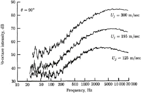
Figure 2.15 – Jet noise spectra at 90º observer angle for three different velocities. (Hubbard, 1991)

The eddies are physically small near the origin of the shear layer and then grow in size downstream of the jet. At some axial location in the jet wake, both small and large scale eddies coexist. The size of this structures can be correlated with the frequency of the noise generation: fine-scales eddies are responsible for high frequency, whilst large scale eddies are of lower frequency.

Since the large eddies contain the bulk of the energy in the turbulent motion, it is expected that control the overall amount of acoustic power. The number and size of these large eddies is dependent upon the manner in which the turbulence is produced. Therefore, the total acoustic power produced by a jet will depend upon the manner in which the turbulence intensity is generated.

While the low-frequency sound end of the power spectrum will depend upon the driving mechanism of the turbulence (since it is produced by the large-scale eddies), the high-frequency sound end of the same spectrum may be independent of the driving forces. The small-scale eddies are associated with rapid fluctuations in the turbulent fluid and they can be thought of as being transported by the large-scale eddies. Thus, the large-scale eddies have some influence on the high-frequency sound, however it is, primarily a Doppler effect which may be neglected for low Mach number turbulence.

2.3.1 Radiation of sound

The acoustic source distribution can be expanded as a Taylor series and the

A point source is called monopole if it is compact and radiates sound equally well in all directions. This radiation is equivalent to that produced by a pulsating sphere, whose radius alternately expands and contracts in a sinusoidal mode. Thus, the monopole source creates a sound wave by introducing and removing fluid alternately into the surrounding area.

The relation between the radiated sound power and the flow parameters when monopole sound is generated by unsteady flow velocities is given by:

(2.16)

where ρ is the specific mass of the gas, the speed of sound, L is the length of the flow in the source region and the flow velocity in the source region.

A point source is called dipole if it is created by superposing two monopoles sources of equal strength, opposite phase, separately by a distance which is much smaller than the wavelength of the sound and equal magnitude. The sound field of a harmonic dipole can be represented as a sphere which oscillates back and forward. It does not radiate sound in all directions equally, where the pressure reaches maxima for angles 0 and 180º, whilst it is dissipated for 90 and 270º.

The dimensional dependence of the dipole sound power in a fluid with a uniform mean density is given by:

(2.17)

A point source is called quadrupole if it is created by superposing two dipoles sources. In this case, there are two principal possibilities: lateral quadrupole and linear quadrupole. In a lateral quadrupole the two dipoles do not lie along the same line. The sound is radiated in front of each monopole source, however, it is cancelled at points equidistant from adjacent opposite monopoles. In a linear quadrupole source, two opposite phase dipoles lie along the same line. In this radiation, there is an evident transition from near to far field.

The dimensional dependence of the radiated quadrupole sound power is given by:

From the equations 2.13, 2.14 and 2.15, it can be seen that the dimensional dependence of the dipole differs by a factor from the power output of the monopole, and the quadrupole differs from the dipole source.

(a) (b)

(c) (d)

Figure 2.16 – Directivity patterns for (a) Monopole, (b) Dipole, (c) Quadrupole (lateral quadrupole) and (d) Quadrupole (linear quadrupole).

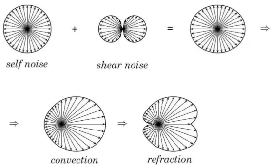
2.3.2 Directional sound pattern in jets

The sound sources are convected downstream by the mean flow. The moving sources tend to radiate more noise in the direction of motion, and this effect is more pronounced at higher speed. This directiveness makes the maximum noise be radiated in directions inclined at observers angles between 30º up to 50º.

Figure 2.17 – Convection effect (Almeida, 2009).

Additionally to the convection effect, the sound generated is affected by refraction. When the wave front propagates to the far-field regions, its path tends to bend away from the jet axis. This effect creates a cone of relative silence downstream of the noise-generating region. (Tam, 1998). Experimentally, the presence of a cone of silence in which the noise intensity drops by more than 20 dB has been demonstrated by Atvars et al (1965).