ISSN 1678-992X
ABSTRACT: The least limiting water range is a soil physical quality indicator, which is useful to predict the optimum water range for plant growth in a given soil and to study the effects of soil use and management over this optimum water range by integrating the effects of available water, penetration resistance and air filled porosity. This study tested six equations to fit water retention and penetration resistance surface responses used to determine the least limiting water range and present a simple algorithm written in the open source software R for fitting, calculation and visualization of the least limiting water range. Five soils from Brazil and Canada, under different use and management conditions were used to test the functions. The results show that the three water retention surface responses had good statistical properties for fitting water retention and that two of the penetration resistance surface responses were adequate to fit the data, while one failed to achieve convergence in two instances. The open source code performed as well as the commercial statistical package SAS for fitting the penetration resistance and water retention equations.
Keywords: nonlinear regression, soil physical quality
Water retention and penetration resistance equations for the least limiting water range
Tairone Paiva Leão1*
Universidade de Brasília/Faculdade de Agronomia e Medicina Veterinária, Campus Darcy Ribeiro – 79910-900 – Brasília, DF – Brasil.
*Corresponding author <[email protected]> Edited by: Silvia del Carmen Imhoff Received August 03, 2017 Accepted October 05, 2017
Introduction
Over the last decades, there has been a search for indicators of soil physical quality able to integrate soil physical parameters in a single index that can be easily measured and correlated with crop production factors (Dexter, 2004; Letey, 1985; Silva et al., 1994). The Least Limiting Water Range (LLWR) is an indicator of soil physical quality and has been used and validated un-der different crop production systems (Lima et al., 2012; Silva et al., 1994; Wu et al., 2003; Zou et al., 2000). The conceptual basis of the LLWR was proposed by Letey (1985), while Silva et al. (1994) developed a mathemati-cal and statistimathemati-cal framework for the application of the concept to soil data. LLWR is sensitive to changes in soil air filled porosity (AFP) and soil resistance to penetra-tion (SR) and integrates the tradipenetra-tional concept of avail-able water defined as the water content between field capacity (FC) and permanent wilting point (PWP) in a particular soil. In the implementation of the method by Silva et al. (1994), AFP, SR, PWP and FC are defined as a function of soil bulk density (Db), thereby creating an index that, once parameterized, can be used for monitor-ing soil physical quality by measurmonitor-ing soil bulk density alone.
The objectives of this research were to: i) evaluate the fitting properties and statistical quality of three soil water retention and three soil resistance to penetration equations to calculate LLWR, and ii) present a code de-veloped in the open source software GNU R (R Develop-ment Core Team, version 3.0.1 “Good Sport”) for fitting the relevant equations and creating a LLWR plot.
Materials and Methods
Mathematically, LLWR quantification is based on the fitting of a water retention function and a soil
pen-etration resistance function. The water retention func-tion, in this particular case, must incorporate soil struc-tural variability, which can be achieved by incorporating soil bulk density into the function. Silva et al. (1994) used a power function described by Ross et al. (1991) for fitting the soil water retention curve:
θ = a ψb (1)
where: θ = volumetric water content (cm3 cm–3), ψ =
soil water potential (MPa) and a and b = empirical pa-rameters.
The “stepwise” multiple regression procedures used by Silva et al. (1994) resulted in a three parameter equations with good statistical properties to characterize the structural influence on the soil water retention pro-cess (Tormena et al., 1999; Betz et al., 1998).
θ = exp(a + b Db) ψc (2)
where: Db = soil bulk density (g cm–3) and a, b, and c =
empirical parameters.
Soil bulk density can also be incorporated into the classic equation of van Genuchten (1980) for the soil wa-ter retention curve:
θ = θr + (θs – θr) / [1 + (αψ)
n](1–1/n) (3)
where: θr = soil residual water content (cm
3 cm–3), θ s =
soil saturated water content (cm3 cm–3), α = inverse of
the air entry water potential value (MPa–1) and n=
em-pirical parameter. To incorporate soil bulk density, the soil saturated water content is replaced by soil total po-rosity, calculated as 1 – Db/Dp, where: Dp = soil particle density, usually assumed as 2.65 g cm–3.
Another form of incorporating Db into Eq. 1 is through the a parameter:
Soils and Plant Nutrition
|
Resear
ch Ar
θ = a0 Dba1ψb (4)
where: a0, a1 and b = empirical parameters. The soil penetration resistance relationship is usually described using the non-linear equation developed by Busscher and Sojka (1987) (Silva et al., 1994):
SR = dθe D
bf (5)
where: SR = soil resistance to penetration (MPa) and d,
e, and f = empirical parameters.
Busscher (1990) evaluated eight equations to fit the soil penetration resistance function and Eq. 5 was the equation with the highest coefficient of determina-tion (R2
average = 0.91) and with a good ratio of the
coef-ficient of determination to the number of empirical pa-rameters. Equation 5 is also mathematically simple and easily implemented in statistical software.
Despite the frequent use of Eq. 5 in studies to quantify LLWR and in soil resistance studies, several equations can be used to fit the soil resistance function, including equations that incorporate other independent variables, such as grain size parameters, water content at a given water potential, organic matter, among others. Perumpral (1987), Busscher (1990) and Caranache (1987) list almost twenty equations that can be used to fit the soil resistance to penetration function.
Ayres and Perumpral (1982) searched for an em-pirical nonlinear equation that was simple, but with good fitting properties to fit SR data as a function of soil water content and dry bulk density. Their procedure re-sulted in a four-parameter equation:
SR = (a Dbb) / [c + (θ – d)2] (6)
where: a, b, c and d = empirical parameters. In their study, Eq. 6 resulted in values of R2 > 0.9 for soils with
clay content ranging from 0 to 1000 g kg–1 (Ayres and
Perumpral, 1982).
Vaz et al. (2001) used a nonlinear three-parameter equation to fit the SR function by simultaneously mea-suring water content and soil penetration resistance us-ing a cone penetrometer adapted with a time domain reflectometry (TDR) sensor:
SR = a(Dbb/D
p) exp(-c θ) (7)
where: a, b, and c = Empirical parameters.
The majority of the equations presented earlier can be linearized by logarithmic transformation. Since it is mathematically and computationally easier to work with linearized equations, many studies have used lin-earized forms of these equations to fit water retention and penetration resistance data (Silva et al., 1994; Betz et al., 1998; Zou et al., 2000). However, in many instances, the linear transformation also involves a transformation of the stochastic term (error), affecting statistical as-sumptions of the model (Bates and Watts, 1988). Besides, techniques and algorithms for nonlinear regression have improved dramatically over the past decades, becoming more efficient and accessible to a greater number of re-searchers (Seber and Wild, 1989). The computing power of most personal devices of today are greater than the machines used in the past and fitting a nonlinear equa-tion has become trivial in terms of processing power and time consumption.
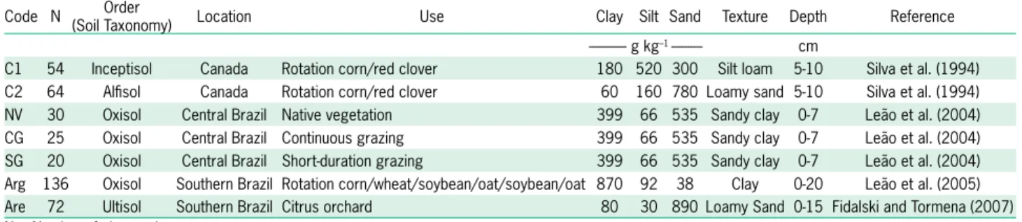
Equations 2 to 7 were evaluated using a dataset compiled and described by Leão et al. (2005). Five soils from different regions, taxonomic classes, grain size dis-tributions and managements were used to evaluate the equations. The basic characterization of soils, including grain size distribution, use and reference is presented in Table 1. The soils used in this research are: a silt loam Inceptisol (Can1), a loamy sand Alfisol (Can2); a sandy clay Oxisol under native vegetation (NV), continuous grazing (CG), and short duration intensive grazing (SG); a clay Oxisol under grain rotation (Arg); and a loamy sand Ultisol under orange orchard (Are) (Table 1).
As several publications deal with the theoretical concept of LLWR (Letey, 1985; Silva et al., 1994) and the procedures for sampling and laboratory analysis to quantify the variables Db, θ, RP and ψ (Klute, 1986; Silva et al., 1994; Betz et al., 1998; Tormena et al., 1999), this research was mainly focused in the data analysis pro-cedures. For model comparison, the equations were fit-ted using SAS software (Statistical Analysis System, ver-sion 9.2) as described by Leão et al. (2005). Afterward, two equations were chosen, one for the water retention curve and the other for the soil penetration resistance
Table 1 − Description of the soils used for testing Eqs. 2 to 7.
Code N Order
(Soil Taxonomy) Location Use Clay Silt Sand Texture Depth Reference --- g kg–1 --- cm
and 0.0008 (cm3 cm–3)2 for Eq. 4. The average R2 value
was approximately 0.85 for Eqs. 2 and 3 and 0.86 for Eq. 4, while the F value was 3808.6, 3817.3 and 3088.8 for Eqs. 2, 3 and 4, respectively (Table 2). This shows that the statistical quality of the fittings was similar. In six cases, one of the parameters was not statistically sig-nificant, as evaluated by the confidence interval of the parameter estimate. The presence of nonsignificant pa-rameters in a nonlinear model may be an indicator that these parameters are superfluous to fit the model to the specific dataset (Ratkowsky, 1990). However, these pa-rameters did not affect the fitting quality and predictive capability of the models, as indicated by data in Table 2. Although it is nearly equivalent to Eqs. 2 and 3, Eq. 4 had fitting quality indicators slightly better than the other two, with slightly lower mean squared error and slightly higher R2. Nonetheless, this model should
be used with caution, especially when simple optimiza-tion methods are used, such as in Leão and Silva (2004). Equation 4 is a more complex model from the nonlinear fitting point of view as the likelihood of dispersion of the parameter surface in the nonlinear regression search procedure is greater. In the case of complex, multipa-rameter and/or intrinsically nonlinear models, more ro-bust search procedures are recommended. One of the best procedures for this purpose is the Levenberg-Mar-quardt procedure (Levenberg, 1944; MarLevenberg-Mar-quardt, 1963). The Levenberg-Marquardt is a robust search procedure that usually converges when the initial parameter value guess is within the expected range and when the model adequately describes the shape of the relationship be-function. A simple code in GNU R (R Development Core
Team, version 3.0.1 “Good Sport”) was developed to fit the equations and plot the LLWR. The fitting properties of the R code were compared to the SAS results.
Results and Discussion
Models comparison
Results from fitting the soil water retention curve functions described by Eqs. 2, 3 and 4 are presented in Table 2. The nonlinear regression procedure achieved convergence for all equations and all soils (p < 0.0001). The main points to be checked in a nonlinear regression fitting, in order of importance, are: 1. the convergence of the model, 2. the significance of the parameters, 3. the probability associated with the F value of the regression analysis of variance, 4. the mean square error, and 5. the
F value. The coefficient of determination, although often regarded as the most important indicator of goodness of fit in regression procedures, is not a reliable indicator in nonlinear regression since the total sum of squares does not add to zero as it is the case in linear regression pro-cedures (Seber and Wild, 1989). Therefore, the R2 values
presented in Tables 1 and 2 should be viewed with cau-tion. These values are not derived from the nonlinear fitting procedure. They were calculated by linear regres-sion of the observed versus predicted values for each model.
Overall, the value of the mean square error was very similar among the models under evaluation, with an average value of 0.00093 (cm3 cm–3)2 for Eqs. 2 and 3
Table 2 − Fitting results for water retention equations.
Soil Equation Convergence MSE F R2 Parameters
Can1 2 Yes, 5 0.000515 4377.43 0.88 a = -1.0254, b = -0.2218ns, c = -0.0820
Can2 2 Yes, 10 0.000894 1130.96 0.87 a = -2.9397, b = 0.3985ns, c = -0.1945
NV 2 Yes, 8 0.000811 968.5 0.80 a = -2.4553, b = 0.7231, c = -0.1161
CG 2 Yes, 9 0.00117 727.78 0.81 a = -3.0952, b = 1.2159, c = -0.1193
SG 2 Yes, 10 0.0011 651.13 0.77 a = -1.7565, b = 0.1243, c = -0.1181
Arg 2 Yes, 8 0.00041 18247.4 0.93 a = -1.9658, b = 0.6037, c = -0.0953 Are 2 Yes, 8 0.00159 557.02 0.87 a = -0.9888ns, b = -1.3919, c = -0.3439
Can1 3 Yes, 5 0.000516 4370.93 0.88 a = 0.2918, b = -0.3118, c = -0.0820 Can2 3 Yes, 10 0.000897 1127.32 0.87 a = 0.0761, b = 0.5787ns, c = -0.1946
NV 3 Yes, 7 0.000806 975.15 0.80 a = 0.1775, b = 0.7149, c = -0.1160
CG 3 Yes, 8 0.00117 723.52 0.80 a = 0.1498, b = 1.4442, c = -0.1194
SG 3 Yes, 13 0.0011 651.17 0.76 a = 0.1939, b = 0.1721ns, c = -0.1181
Arg 3 Yes, 7 0.000408 18315 0.93 a = 0.2552, b = 0.6757, c = -0.0952
Are 3 Yes, 11 0.00159 557.86 0.88 a = 0.1218, b = -2.3569, c = -0.3439 Can1 4 Yes, 14 0.000611 3685.16 0.85 θr = 0.2031, α = 359.1, n = 1.2406 Can2 4 Yes, 9 0.00113 892.99 0.84 θr = 0.1040, α = 661.2, n = 1.4958 NV 4 Yes, 11 0.00101 777.47 0.76 θr = 0.2096, α = 1907.2ns, n = 1.6084
CG 4 Yes, 11 0.000993 854.8 0.83 θr = 0.2352, α = 646.8, n = 1.6991 SG 4 Yes, 5 0.000594 1208.59 0.87 θr = 0.2413, α = 240.1, n = 1.8421 Arg 4 Yes, 8 0.000581 12848.4 0.90 θr =0.2966, α = 502.9, n = 1.5148 Are 4 Yes, 10 0.000671 1354.46 0.95 θr = 0.0583, α = 199.8, n = 2.4614
tween dependent and independent variables (Leão et al., 2005). As with any nonlinear search procedure, when the Levenberg-Marquardt method is used, the user should check for the possibility of local minima in the procedure convergence (Seber and Wild, 1989). The fitting proce-dure for Eq. 4 should follow the recommendations to fit the van Genucthen (1980) water retention equation from which it derives. Equations 2 and 3 are intrinsically linear and therefore the fitting is somewhat trivial.
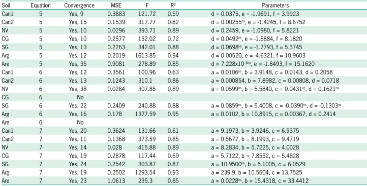
Analysis of soil resistance to penetration equations (Eqs. 5 to 7) showed that Eqs. 5 and 7 had a very simi-lar performance with mean values of the mean squared error of 0.31 and 0.34 MPa2, and F values of 457 and
410, respectively, and R2 of 0.81 in both cases (Table
3). Equation 5 was slightly better than Eq. 7 when the mean squared error and F value are considered. Eq. 6 had an overall lower mean squared error and higher R2 and F; however, it failed to converge in two
condi-tions, namely CG and Are, indicating that this model can be problematic in some cases and should be used with caution. The increase in the number of empirical parameters is known to cause difficulties in the nonlin-ear snonlin-earch procedure and/or dispersion of the parameter surface in the search procedure (Seber and Wild, 1989). This can be minimized by changing the initial values of the parameters thereby avoiding dispersion of the search procedure in the first iterations of the process. In this particular case, the initial values of the parameters were the same for all soils and conditions to evaluate the mod-els in similar conditions. If convergence is not achieved, even if the initial parameter values are altered, this can
be an indicator that the equation does not conform to the data or that there is an excess of empirical param-eters, and this overparameterization can be very problem-atic when nonlinear models are used (Ratkowsky, 1990). Therefore, the use of Eqs. 5 or 7 is recommended to fit soil penetration resistance data.
Code development in GNU R
Based on the model evaluation above, a code in GNU R environment was developed to fit and calculate LLWR. Previously, Leão and Silva (2004) and Leão et al. (2005) developed algorithms to calculate LLWR in commercial software programs, which are usually ex-pensive and often unavailable to public research and education institutions in developing countries. The R system is a free software program developed under the GNU General Public License system, based on the S programming language and can be downloaded for free at http://www.R-project.org. A dataset in *.dat format was used in the analysis. The dataset, called llwr.dat for illustrative purposes, is formatted as shown in Table 4, where Site is the treatment or soil, Db is the soil bulk density (g cm–3), q is the volumetric water content (cm3
cm–3), SR is soil resistance to penetration (MPa) and Y
soil water potential (MPa). To import the file into the program, the following line of code can be used:
llwr<-read.table(“C:/llwr.txt”, header=T, sep=”\t”)
The options header and sep indicate that the first line of the file corresponds to the declaration of
vari-Table 3 − Fitting results for the penetration resistance equations.
Soil Equation Convergence MSE F R2 Parameters
Can1 5 Yes, 9 0.3883 121.72 0.59 d = 0.0375, e = -1.9691, f = 3.9923 Can2 5 Yes, 15 0.1539 317.77 0.82 d = 0.00255ns, e = -1.4245, f = 8.6752
NV 5 Yes, 10 0.0296 393.71 0.89 d = 0.2459, e = -1.0980, f = 5.8221 CG 5 Yes, 10 0.2577 132.02 0.72 d = 0.0492ns, e = -1.6884, f = 8.1820
SG 5 Yes, 13 0.2263 342.01 0.88 d = 0.0698ns, e = -1.7793, f = 5.3745
Arg 5 Yes, 12 0.2019 1613.85 0.94 d = 0.00520, e = -4.6321, f = 10.9603 Are 5 Yes, 35 0.9081 278.89 0.85 d = 7.228x10⁻⁶ns, e = -1.8493, f = 15.1620
Can1 6 Yes, 12 0.3561 100.96 0.63 a = 0.0106ns, b = 3.9148, c = 0.0143, d = 0.2058
Can2 6 Yes, 13 0.1243 310.1 0.86 a = 0.000854, b = 7.8982, c = 0.00808, d = 0.0718 NV 6 Yes, 38 0.0284 307.85 0.89 a = 0.0599ns, b = 5.5840, c = 0.0431ns, d = 0.1621ns
CG 6 No
SG 6 Yes, 22 0.2409 240.88 0.88 a = 0.0859ns, b = 5.4008, c = -0.0390ns, d = -0.1303ns
Arg 6 Yes, 16 0.178 1377.59 0.95 a = 0.0102, b = 10.8915, c = 0.00367, d = 0.2414
Are 6 No
Can1 7 Yes, 20 0.3624 131.66 0.61 a = 9.1973, b = 3.9246, c = 6.9375 Can2 7 Yes, 11 0.1368 373.59 0.85 a = 0.5677, b = 8.1993, c = 9.4719 NV 7 Yes, 14 0.028 415.88 0.89 a = 8.2834, b = 5.7225, c = 4.0028 CG 7 Yes, 19 0.2878 117.44 0.69 a = 5.7122, b = 7.8552, c = 5.4828 SG 7 Yes, 24 0.2542 303.87 0.87 a = 10.9500ns, b = 5.1005, c = 6.0529
Arg 7 Yes, 19 0.2502 1293.54 0.93 a = 239.9, b = 10.5604, c = 13.7525 Are 7 Yes, 23 1.0613 235.3 0.85 a = 0.0228ns, b = 15.4318, c = 33.4412
ables names and that the data are separated by tabu-lation. The configurations for file format and separator can be easily changed according to the user’s require-ments. The analysis can be performed in each treatment at a time, in this case the “Are” treatment, referring to the loamy sand Ultisol was used (Table 1):
attach(llwr)
areia<-llwr[which(Site==”Are”),] detach(llwr)
The commands attach and detach are used to make objects within dataframes accessible to R in fewer key-strokes. In simple terms, they assign or remove data from the program memory for immediate use. For adjusting the equations, the file created for the “Are” dataset, called
areia, is assigned to the program memory. The soil water retention curve is then adjusted using the nls command. Equation 2 was used in the fitting procedure for simplic-ity. The initial values for parameters a, b and c are speci-fied in the command start. The command summary pro-vides the results of the nonlinear fitting procedure:
attach(areia)
areia.cra<-nls(q~exp(a+b*Db)*Y^c, start=list(a=-0.1,b=-0.1,c=-0.1))
summary(areia.cra)
The same procedure is repeated for the soil pen-etration resistance procedure. Equation 5 was used for simplicity:
areia.crp<-nls(SR~d*Db^e*q^f, start=list(d=0.1,e=-0.1,f=0.1))
summary(areia.crp)
The results from the nonlinear procedure for the water retention curve equation are presented below:
Formula: q ~ exp(a + b * Db) * Y^c
Parameters:
Estimate Std. Error t value Pr(>|t|) a -0.98879 0.82347 -1.201 0.23395 b -1.39192 0.48511 -2.869 0.00546 ** c -0.34389 0.01997 -17.218 < 2e-16 ***
---Signif. codes: 0 ‘***’ 0.001 ‘**’ 0.01 ‘*’ 0.05 ‘.’ 0.1 ‘ ’ 1
Residual standard error: 0.03991 on 69 degrees of free-dom
Number of iterations to convergence: 7 Achieved convergence tolerance: 5.214e-06
As discussed before, the values of initial param-eters for the nonlinear regression can and should be al-tered according to the units of each variable to which it corresponds and in case the procedure does not con-verge. Lack of convergence indicates that the search mechanism did not find a reasonable result for the pa-rameter set. Nonlinear equations where convergence is not met should not be used to predict or model data. The results show that convergence was achieved in 7 itera-tions and that the values are almost identical to those found in SAS software (Table 2). The values for the soil penetration resistance surface fitting were also very sim-ilar to those found in SAS:
Formula: SR ~ d * Db^e * q^f Parameters:
Estimate Std. Error t value Pr(>|t|) d 7.228e-06 8.776e-06 0.824 0.413
e 1.516e+01 1.958e+00 7.745 5.86e-11 *** f -1.849e+00 1.776e-01 -10.415 8.52e-16 ***
---Signif. codes: 0 ‘***’ 0.001 ‘**’ 0.01 ‘*’ 0.05 ‘.’ 0.1 ‘ ’ 1 Residual standard error: 0.9529 on 69 degrees of free-dom
Number of iterations to convergence: 31 Achieved convergence tolerance: 6.573e-06
To generate values of the volumetric water contents at the critical limits of LLWR, the datasets containing the parameter values estimated by the two equations must be combined to the original data. This can be done by trans-forming the parameter vector into columns by using the command rbind on the fitting parameters data extracted using the coef command. The command merge combines the two datasets. The new dataset is then attributed to the program memory using the command attach:
areia.crp.coef<-rbind(coef(areia.crp)) areia.cra.coef<-rbind(coef(areia.cra))
areia.coefs<-merge(areia.crp.coef, areia.cra.coef) areia.all<-merge(areia, areia.coefs)
detach(areia) attach(areia.all)
The critical value of the volumetric water content at the FC (qfc) is generated by replacing the water po-tential at the FC in Eq. 2, |0.01| MPa in this case. For the critical value of volumetric water content at the PWP (qpwp), the value of water potential of |1.5| MPa was used:
areia.all$qfc<-exp(areia.all$a+areia.all$b*areia. all$Db)*0.01^areia.all$c
Table 4 – Model for the input datafile used in R software.
Site Db Q SR Y
SG 1.2957 0.3299 1.289868 0.01
SG 1.324 0.3223 2.894777 0.03
SG 1.3381 0.2552 4.111531 1.5
SG 1.3551 0.2313 4.768208 1.5
SG 1.3559 0.4022 2.25171 0.006
areia.all$qpwp<-exp(areia.all$a+areia.all$b*areia. all$Db)*1.5^areia.all$c
The critical volumetric water content where AFP is 10 % is calculated as:
θa = (1 – Db/Dp) – 0.1 8
where: Dp is the particle density (g cm–3) assumed as
2.65 g cm–3:
areia.all$qafp<-(1-(areia.all$Db/2.65)-0.1)
The new variables created by the equations above are assigned to the dataset specifying the name of the dataset open, followed by the symbol “$” and the name of the new variable. Therefore, to generate the vari-able qafp, the command areia.all$qa should be speci-fied. The same procedure can be used on the variables open for manipulation in the dataset, one example is the code fragment areia.all$Db. The critical volumetric water content where the SR is equal to 2 MPa (qsr) is calculated by replacing this value into Eq. 5 and solv-ing for volumetric water content. The critical value can be easily changed to a value different from 2 MPa, ac-cording to the user’s requirements.
areia.all$qsr<-((2/(areia.all$d*areia.all$Db^areia. all$e))^(1/areia.all$f))
LLWR plot can be produced with the following code fragment:
attach(areia.all) par(mar=c(4,4.5,2,1)) par(oma=c(0,0,0,0))
plot(Db,qfc, col = “blue”, type = “b”, xlim = c(1.45,1.85), ylim=c(0.0,0.3),lwd=2,
xlab=expression(paste(“Soil Bulk Density, g cm”^”-3”)), ylab=expression(paste(“Volumetric Water Content, cm”^{3}, “cm”^{-3})))
lines(Db,qafp, col = “orange”, type=”b”, lwd=2, pch=2)
lines(Db,qsr, col = “green”, type=”b”, lwd=2, pch=2) lines(Db,qpwp, col = “red”, type=”b”, lwd=2, pch=2) legend(“topleft”, legend=c(“FC”, “PWP”, “SR”, “AFP”), cex=1, col=c(“blue”, “red”, “green”, “orange”), lty=1:3, lwd=2, bty=”n”)
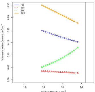
The command par is only necessary when there are size configuration problems in the window where the plot is shown. The commands in R should be exe-cuted line by line, the execution of the code as a whole is not recommended until the user becomes more proficient with the procedure and the software. By executing each step at a time, the user can check for problems and inconsistencies in the fitting and plotting procedures. Figure 1 shows the procedure results. The
axis, fonts, lines, colors and other configurations can be easily modified according with the preferences of the user.
The Db value, where LLWR = 0, called the criti-cal bulk density (Dbc), can also be calculated in R. A
simple optimization procedure is used. The equation to be optimized is the equation of the superior limit minus the inferior LLWR limit. The equations that intercept at the critical limit can be easily identified by inspect-ing the LLWR plot (Figure 1). The equation should be specified with the values of the coefficients obtained from the nonlinear regression procedure. In the case of the areia dataset, Dbc corresponds to the intersection of the lines of the volumetric water content at field capac-ity and the water content in which the soil penetration resistance is equal to 2 MPa. In R, the critical bulk den-sity was specified as the Dbc function, where x is the value of the critical bulk density to be optimized. The command uniroot performs the optimization in the Db limits between 0.0 and 2.0 g cm–3:
Dbc<-function(x) exp(-0.98-1.39*x)*(0.01^-0.34)-((2/ (0.000007*x^15))^(1/-1.84))
uniroot(Dbc, c(0,2))
As a result, the critical bulk density where LLWR = 0 is estimated:
$root [1] 1.820318
The last step is to add a line corresponding to Dbc into the graph. This can be specified by the command:
abline(v=1.820318, col =”black”)
Figure 1 − Least limiting water range plot generated using R
Conclusions
All water retention equations performed well in fit-ting to the observed data. For the penetration resistance data, Eqs. 5 and 7 performed similarly well, while Eq. 6 failed to converge in two occasions. These equations can be combined to determine the least limiting water range. A simple GNU R application was also developed to quantify the least limiting water range. The results from the application were very similar to those found using a commercial software program widely used in statistical analyses. As R is a very flexible programming language, the code fragments presented in this study can be promptly modified to suit the needs of different data-sets, models as well as for data manipulation.
References
Ayres, P.D.; Perumpral, J.V. 1982. Moisture and density effect on cone index. Transactions of ASAE 25: 1169-1172.
Bates, D.M.; Watts, D.G. 1988. Nonlinear Regression Analysis and its Applications. John Wiley, New York, NY, USA. Betz, C.L.; Allmaras, R.R.; Copeland, S.M.; Randall, G.W.
1998. Least limiting water range: traffic and long-term tillage influences in a Webster soil. Soil Science Society of America Journal 62: 1384-1393.
Busscher, W.J.; Sojka, R.E. 1987. Enhancement of subsoiling effect on soil strength by conservation tillage. Transactions of ASAE 30: 888-892.
Busscher, W.J. 1990. Adjustment of flat-tipped penetrometer resistance data to a common water content. Transactions of ASAE 33: 519-524.
Caranache, A. 1987. PENETR: a generalized semi-empirical model estimating soil resistance to penetration. Soil and Tillage Research 19: 51-70.
Dexter, A.R. 2004. Soil physical quality. Part I. Theory, effects of soil texture, density, and organic matter, and effects on root growth. Geoderma 120: 201-214.
Fidalski, J.; Tormena, C.A. 2007. Homogeneity of soil physical quality in-between rows of an orange orchard with groundcover systems. Revista Brasileira de Ciência do Solo 31: 637-645 (in Portuguese, with abstract in English).
Klute, A. 1986. Water retention: laboratory methods. p. 635-660. In: Klute, A., ed. Methods of soil analysis: physical and mineralogical methods. American Society of Agronomy, Madison, WI, USA.
Leão, T.P.; Silva, A.P.; Macedo, M.C.M.; Imhoff, S.; Euclides, V.P.B. 2004. Least limiting water range in continuous and short duration grazing systems. Revista Brasileira de Ciência do Solo 28: 1-8 (in Portuguese, with abstract in English).
Leão, T.P.; Silva, A.P. 2004. A simplified Excel® algorithm for estimating the least limiting water range of soils using nonlinear regression. Scientia Agricola 61: 649-654.
Leão, T.P.; Silva, A.P.; Perfect, E.; Tormena, C. 2005. An algorithm for calculating the least limiting water range of soils. Agronomy Journal 97: 1210-1215.
Letey, J. 1985. Relationship between soil physical properties and crop production. Advances in Soil Science 1: 277-294. Levenberg, K. 1944. A method for the solution of certain
non-linear problems in least squares. Quarterly of Applied Mathematics 2: 164-168.
Lima, C.L.R.; Miola, E.C.C.; Timm, L.C.; Pauletto, E.A.; Silva, A.P. 2012. Soil compressibility and least limiting water range of a constructed soil under cover crops after coal mining in southern Brazil. Soil and Tillage Research 124: 190-195. Marquardt, D. 1963. An algorithm for least-squares estimation of
nonlinear parameters. SIAM Journal on Applied Mathematics 11: 431-441.
Perumpral, J.V. 1987. Cone penetrometer applications: a review. Transactions of the American Society of Agricultural Engineers 30: 939-944.
Ratkowsky, D.A. 1990. Handbook of Nonlinear Regression Models. Marcel Dekker, New York, NY, USA.
Ross, P.J.; Williams, J.; Bristow, K.L. 1991. Equations for extending water-retention curves to dryness. Soil Science Society of America Journal 55: 923-927.
Seber, G.A.F.; Wild, C.J. 1989. Nonlinear Regression. John Wiley, New York, NY, USA.
Silva, A.P.; Kay, B.D.; Perfect, E. 1994. Characterization of the least limiting water range of soils. Soil Science Society of America Journal 58: 1775-1781.
Tormena, C.A.; Silva, A.P.; Libardi, P.L. 1999. Soil physical quality of a Brazilian Oxisol under two tillage systems using the least limiting water range approach. Soil and Tillage Research 52: 223-232.
van Genuchten, M.Th. 1980. A closed form equation for predicting the hydraulic conductivity of unsaturated soils. Soil Science Society of America Journal 44: 892-898.
Vaz, C.M.P.; Bassoi, L.H.; Hopmans, J.W. 2001. Contribution of water content and bulk density to field soil penetration resistance as measured by a combined cone penetrometer-TDR probe. Soil and Tillage Research 60: 35-42.
Wu, L.; Feng, G.; Letey, J.; Ferguson, L.; Mitchell, J.; McCullough-Sanden, B.; Markegard, G. 2003. Soil management effects on the nonlimiting water range. Geoderma 114: 401-414. Zou, C.; Sands, R.; Buchan, G.; Hudson, I. 2000. Least limiting